Accidental Cameras: Creating Images from Shadows
by
Vickie Ye
Submitted to the Department of Electrical Engineering and Computer
Science
in partial fulfillment of the requirements for the degree of
Master of Engineering
at the
MASSACHUSETTS INSTITUTE OF TECHNOLOGY
February 2018
c
○ Massachusetts Institute of Technology 2018. All rights reserved.
Author . . . .
Department of Electrical Engineering and Computer Science
February 1, 2018
Certified by . . . .
William T. Freeman
Professor
Thesis Supervisor
Accepted by . . . .
Christopher J. Terman
Chairman, Department Committee on Graduate Theses
Accidental Cameras: Creating Images from Shadows
by
Vickie Ye
Submitted to the Department of Electrical Engineering and Computer Science on February 1, 2018, in partial fulfillment of the
requirements for the degree of Master of Engineering
Abstract
In this thesis, we explore new imaging systems that arise from everyday occlusions and shadows. By modeling the structured shadows created by various occlusions, we are able to recover hidden scenes. We explore three such imaging systems. In the first, we use a wall corner to recover one-dimensional motion in the hidden scene be-hind the corner. We show experimental results using this method in several natural environments. We also extend this method to be used in other applications, such as for automotive collision avoidance systems. In the second, we use doorways and spheres to recover two-dimensional images of a hidden scene behind the occlusions. We show experimental results of this method in simulations and in natural environ-ments. Finally, we present how to extend this approach to infer a 4D light field of a hidden scene from 2D shadows cast by a known occluder. Using the shadow cast by a real house plant, we are able to recover low resolution light fields with different levels of texture and parallax complexity.
Thesis Supervisor: William T. Freeman Title: Professor
Contents
1 Introduction 15
1.1 Related Work in Non-Line-of-Sight (NLOS)
Imaging . . . 16
1.2 Contributions and Outline . . . 18
2 General Imaging System 19 2.1 Light Transport Model . . . 19
2.2 Inference . . . 22
3 Corner Cameras: Reconstructing Motion in One Dimension 25 3.1 Model . . . 26
3.2 Method . . . 26
3.3 Implementation Details . . . 29
3.4 Experiments and Results . . . 30
3.4.1 Environments . . . 30
3.4.2 Video Quality . . . 32
3.4.3 Estimated Signal Strength . . . 33
4 Extensions of the Corner Camera 37 4.1 Reconstruction with a moving observer . . . 37
4.1.1 Problems of a Moving Camera . . . 37
4.1.2 Real-time system . . . 39
4.2.1 Recovering Depth with Adjacent Corner Cameras . . . 41
4.2.2 Experiments and Results . . . 43
5 Reconstructing in Two Dimensions 47 5.1 Spherical Occluders . . . 47
5.1.1 Inference . . . 49
5.1.2 Experimental Results . . . 50
5.2 Rectangular Occlusions . . . 52
5.2.1 Experimental Results . . . 53
6 Recovering 4D Light Fields 57 6.1 Method . . . 58
6.1.1 Light Field Model . . . 58
6.1.2 Light Field Inference . . . 59
6.1.3 Occluder Calibration . . . 60
6.2 Experimental Reconstructions . . . 61
7 Conclusion 63 A Additional Derivations 65 A.1 Simple Perturbation Model . . . 65
A.1.1 Photometric signal of the corner camera . . . 66
A.1.2 Intensity contributions of the subject of brightness C . . . 68
A.1.3 Final Model . . . 71
A.1.4 Examples . . . 72
A.1.5 Rate of signal decay as person moves away from corner . . . . 73
A.2 Temporal Smoothing for the Corner Camera . . . 74
A.3 Derivation of the Light Field Prior . . . 75
A.3.1 Reparameterization of light fields . . . 76
A.3.2 Dimensionality gap of 4D light fields . . . 77
List of Figures
1-1 We show an example in which information from the scene hidden be-hind the wall corner can be recovered, using the visible observations at the base of wall corner. (A) show that the light from the hidden scene casts structured shadows on the floor at the base of the corner. This is similar to how, from the point of view of an observer walking around the occluding edge (along the magenta arrow), light from dif-ferent parts of the hidden scene becomes visible at difdif-ferent angles (B). This subtle variation is not perceptible to the naked eye, such as in (C), but is present, and can be computationally extracted as it is in (D). 15
2-1 We show the various ways the light from the hidden scene can be parameterized, depending on the occluder we use. In (A), we show a system in which the wall corner allows us to recover the 1D angular projection of the scene behind the corner. We parameterize the hidden scene in 1D, as a function of the angle from the wall. In (B), we show a system in which the doorway occluder allows us to recover two dimensions of information. We parameterize the hidden scene in 2D, as a function of position in a plane in the scene. . . 21
2-2 (A) We show an example observation for the edge camera introduced in 1. In this case, the occluder is the wall edge, which focuses light from the hidden scene behind the corner onto the observation plane at the base of the wall edge. In (B), we show the response of the system to a single point light source in the middle of our scene. The impulse responses of the system for all such desired reconstruction pixels form the columns of the light transport matrix A. In (C) we visualize the row of the estimation gain matrix that recovers the light source of (B) from the observations. . . 22
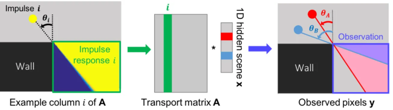
3-1 We show our linear model of the corner camera. On the left, we show an example column of the light transport matrix A, which is built from the impulse responses of the system for each element of x. The resulting A transforms the scene parameters x into the observed pixels y. . . 27 3-2 We show a result in which two people, one red and one black, walk
around, illuminated by a large diffuse light, in an otherwise dark room. The resulting trajectories of their motion therefore show the colors of their clothing. . . 30 3-3 One-dimensional reconstructed videos of indoor, hidden scenes.
Re-sults are shown as space-time images for sequences where one or two people were walking behind the corner. In these reconstructions, the angular position of a person, as well as the number of people, can be clearly identified. Bright line artifacts are caused by additional shad-ows appearing on the penumbra. . . 31 3-4 1-D reconstructed videos of a common outdoor, hidden scene under
various weather conditions. Results are shown as space-time images. The last row shows results from sequences taken while it was beginning to rain. Although artifacts appear due to the appearing raindrops, motion trajectories can be identified in all reconstructions. . . 32
3-5 The result of using different cameras on the reconstruction of the same sequence in an indoor setting. Three different 8-bit cameras (an iPhone 5s, a Sony Alpha 7s SLR, and an uncompressed RGB Point Grey) si-multaneously recorded the carpeted floor. Each camera introduced a different level of per-pixel sensor noise. The estimated standard devia-tion of sensor noise, 𝜆, is shown in (B). We compare the quality of two sequences in (C) and (D). In (C), we have reconstructed a video from a sequence of a single person walking directly away from the corner from 2 to 16 feet at a 45 degree angle from the occluded wall. This experiment helps to illustrate how signal strength varies with distance from the corner. In (D), we have done a reconstruction of a single person walking in a random pattern. . . 33
3-6 Calculation of the contribution to the brightness of the target. Region 1 is the umbra region of the observation plane; none of the cylinder is visible from region 1, and thus its intensities do not change after introducing the target to the scene. Region 2 is the penumbra region; in region 2, part of the cylinder is visible. In region 3, the entire cylinder is visible. . . 34
4-1 We show the reconstructed trajectories of the hidden scene, for a mov-ing camera observer. We show results for two scenarios. In the top panel, the observation plane is a tiled surface; in the bottom, it is carpeted. The tile surface is more reflective, and shows noticeable changes in the brightness of the reconstruction as the camera viewing angle changes. The carpet shows a less dramatic effect. Horizontal line artifacts in both reconstructions are due to misalignment between the current frame and the mean frame. . . 39
4-2 Here we show an example of the usage of the real-time corner camera. In the left panel, we show the hidden scene of a girl behind a corner. In the middle panel, we show the interactive calibration window, in which the user selects the corner and observation region on the ground. In the right panel, we show snapshots of the real-time output at three different times. In each frame, we see a later part of the trajectory being added to the right of the space-time image. . . 40 4-3 (A) The four edges of a doorway contain penumbras that can be used
to reconstruct a 180∘ view of a hidden scene. Parallax occurs in the reconstructions from the left and right wall. (B) A hidden person will introduce an intensity change on the left and right wall penum-bras at angles 𝜑(𝑡)𝐿 and 𝜑(𝑡)𝑅. We can recover the hidden person’s two-dimensional location using Eq. 4.2. . . 41 4-4 The four edges of a doorway contain penumbras that can be used to
reconstruct a 180∘ view of a hidden scene. The top diagram indicates the penumbras and the corresponding region they describe. Parallax occurs in the reconstructions from the left and right wall. This can be seen in the bottom reconstruction of two people hidden behind a doorway. Numbers/colors indicate the penumbras used for each 90∘ space-time image. . . 42 4-5 We performed controlled experiments to explore our method to infer
depth from stereo edge cameras. A monitor displaying a moving green line was placed behind an artificial doorway (A) at four locations: 23, 40, 60, and 84 cm, respectively. (B) shows reconstructions done of the edge cameras for the left and right wall when the monitor was placed at 23 and 84 cm. Using tracks obtained from these reconstructions, the 2-D position of the green line in each sequence was estimated over time (C). The inferred position is plotted with empirically computed error ellipses (indicating one standard deviation of noise). . . 43
4-6 The results of our stereo experiments in a natural setting. A single person walked in a roughly circular pattern behind a doorway. The 2-D inferred locations over time are shown as a line from blue to red. Error bars indicating one standard deviation of error have been drawn around a subset of estimates. Our inferred depths capture the hidden subject’s cyclic motion, but are currently subject to large error. . . . 44
5-1 We show a schematic of an imaging setup used for the spherical oc-cluder. In (A), we show a sphere in between the observation plane and two colored cylinders. The camera can see the observation plane, but the two cylinders are out of sight. In (B) we show the discrete parameterization of the light from the hidden scene. We choose a grid parallel to the observation plane, placed at a known depth. The 𝑖-th column of the transport matrix will be the observed shadow from a point source placed at the 𝑖-th location on this grid. . . 48
5-2 (A) An image of the observation plane behind a sphere and scene. The sphere creates a shadow on the observation plane that contains infor-mation about the scene behind it. (B) The response of the system to a single point light source in the middle of our scene. These im-pulse responses form the columns of our transfer matrix A. (C) The estimation gain image of middle pixel in our scene. Namely, the 𝑖-th estimation gain image shows what information in the observation is used to reconstruct the 𝑖-th pixel in the scene. . . 49
5-3 We show results for our first experimental scenario. In (A), we show the setup: we project the hidden scene from a monitor onto a blank observation wall, four feet away. A 9 inch soccer ball sits halfway between the two. In (B), we show the hidden scenes we project from the monitor, and in (C), we show the resulting reconstructions. . . 51
5-4 We show results for our second experimental setup. On the left, we show the camera capturing a white wall, with a soccer ball placed 2 feet away from it. The hidden scene consists of two simple paper objects, and is illuminated by a large diffuse light, as well as ambient lighting in the room. We show reconstructions of the two hidden objects placed at two depths. On the left, the two objects are placed 5 feet away from the observation wall, and on the right, they are placed 4.5 feet away from the wall. . . 52 5-5 We show the imaging setup for imaging a hidden scene through a
door-way, from the shadow on the ceiling. In (A), we show two colored cylinders outside a room, casting structured shadows onto the ceiling. The camera sees the ceiling, but cannot see outside the room. In (B), we choose to represent the hidden scene as grid of point sources on a 2D plane placed above the scene at a known height, parallel to the ceiling. The 𝑖-th column of the transport matrix will be the observed shadow from a point source at the 𝑖-th location on this grid. . . 53 5-6 We show the experimental results for our first scenario, shown in the
leftmost panel. A rectangular occluder is placed 2ft way from the observation plane; a hidden object shown in the second panel is placed at various distances away from it. We show reconstructions of the object placed 5ft away from the wall (third panel) and 6ft away from the wall (right-most panel). . . 53 5-7 We show the experimental results for our second scenario: imaging a
hidden scene outside a doorway. The camera inside the dark room sees the ceiling, and cannot see the scene outside the door. We reconstruct two scenes. The first scene is of two covered chairs, one green and one white, placed a few feet from the door. The second is of a man wearing orange, standing in the same location (the hidden scene is viewed from through the doorway). . . 54
6-1 a) The simplified 2D scenario. The scenario depicts all the elements of the scene (occluder, hidden scene and observation plane) and the parametrization planes for the light field (dashed lines). In (b) we show the discretized version of the scenario, with the light field and the observation encoded as the discrete vectors x and y, respectively. The transfer matrix is a sparse, row-deficient matrix that encodes the occlusion and reflection in the system. . . 58 6-2 Experimental setup used to calibrate complex occluders. An impulse
at a single position on an LCD screen placed at scene plane casts a shadow. This shadow is used to compute the visibility function of that scene position and all observation positions. This process is done for each scene position. . . 60 6-3 Reconstructions of an experimental scene with two rectangles, one blue
at 𝑎 = 0 and one red at 𝑎 = 0.5. (a) Schematic of the system setup. (b) Observation plane after background subtraction. (c) Six views of the true scene, shown to demonstrate of what the true light field would look like. These are taken with a standard camera from equivalent positions on the observation wall. The “camera” moves right as we move left to right on the grid, and down as we move top to bottom on the grid. (d) These selected views of the reconstructed light field. . . 61 6-4 Reconstructions of an experimental scene with a single subject, seated
at the scene plane. (a) Observation plane after background subtraction. (b) Six views of the true scene, captured in the same manner as in Fig. 6-3 (c) Reconstructions of the light field for the same views as in (b). . . 62
A-1 Simple model of a corner camera. We seek formulas for the image intensities at a point (𝑥, 𝑦) in the observation plane. We have a wall of brightness 𝐵, a subject of brightness 𝐶, and a uniform background of brightness 𝐴. . . 66
A-2 Brightness contribution of one patch of the wall to the brightness of the ground plane depends on the angle between the red arrow and the ground’s surface normal. . . 67 A-3 Calculation of the contribution to the brightness of the subject. . . . 68 A-4 The result of imposing temporal smoothness or averaging adjacent
frames in time to help in reducing noise. . . 75 A-5 Light field reparameterization by a displacement of the scene plane.
Chapter 1
Introduction
Although often not visible to the naked eye, in many environments, light from ob-scured portions of a scene is scattered over many of the observable surfaces. In certain cases, we can exploit the structured distribution of this light to recover information about the hidden scene. As an example, consider the scenario depicted in Figure 1(A).
Figure 1-1: We show an example in which information from the scene hidden behind the wall corner can be recovered, using the visible observations at the base of wall corner. (A) show that the light from the hidden scene casts structured shadows on the floor at the base of the corner. This is similar to how, from the point of view of an observer walking around the occluding edge (along the magenta arrow), light from different parts of the hidden scene becomes visible at different angles (B). This subtle variation is not perceptible to the naked eye, such as in (C), but is present, and can be computationally extracted as it is in (D).
observer, we see in 1(A) and (D) that the light observed on the ground at the base of the corner shows subtle variations that reveal information about the elements behind the corner. From a point near the wall, very little of the hidden scene is visible, and the ground reflects little light from beyond the corner. However, as we move around the corner, along the magenta arrow, the ground begins to reflects red light as A becomes visible, and then purple light as both A and B become visible. This can be seen from the point of view of an observer at the corner in Figure 1(B); as the observer moves along the magenta arrow around the corner, she sees an increasing amount of the scene until eventually, the hidden scene comes fully into view.
We can then think of the shadow we see on the ground as really the sum of several distinct shadows caused by light from various regions in the scene. In this way, the vertical edge occlusion of the wall corner acts as an aperture that filters light from beyond the corner. We can therefore think of the optical system of Figure 1(A) as an accidental camera [21] for the out-of-sight region.
1.1
Related Work in Non-Line-of-Sight (NLOS)
Imaging
The ability to image such scenes not directly in the line of sight would prove useful in a wide range of applications, from search-and-rescue, to anti-terrorism, to road traffic and collision avoidance [3]. However, this problem is very difficult. In this section we describe previous non-line-of-sight (NLoS) methods. Previous methods used to see past or through occluders have ranged from using WiFi signals [1] to exploiting random specular surfaces [27, 8]. In this summary, we emphasize two primary approaches that have been used to see past occluders and image hidden scenes.
Time-of-Flight Sensors: Past approaches to see around corners have largely involved using time-of-flight (ToF) cameras [19, 26, 13]. These methods involve using a laser to illuminate a point that is visible to both the observable and hidden scene,
and measuring how long it takes for the light to return [26, 20]. By measuring the light’s time of flight, one can infer the distance to objects in the hidden scene, and by measuring the light’s intensity, one can often learn about the reflectance and curvature of the objects [18]. Past work has used ToF methods to infer the location [11], size and motion [17, 9], and shape [22] of objects in the hidden scene. These methods have also been used to count hidden people [25].
ToF cameras work well in estimating the depths of hidden objects, however, they have a number of limitations. First, they require specialized and comparatively ex-pensive detectors with fine temporal resolution. Second, they are limited in how much light they can introduce in the scene to support imaging. Third, they are vulnerable to interference from ambient light sources. Unlike passive methods, which make use of ambient illumination, ToF systems must introduce every photon that is measured. By contrast, our proposed passive technique operates in unpredictable indoor and outdoor environments with comparatively inexpensive consumer cameras.
Imaging Using RGB Videos: Other work has previously considered the possi-bility of using structures naturally present in the real world as cameras. Naturally occurring pinholes (such as windows) or pinspecks have been previously used for non-line-of-sight imaging [21, 7]. In addition, specular reflections off of human eyes have been used to image hidden scenes [16]. Although these accidental cameras can be used to reconstruct 2-D images, they require a more specialized accidental camera scenario than the simple edges we propose to use in this work.
Our work also bears some resemblance to [24], which focuses on detecting and visualizing small, often imperceptible, color changes in video. However, in our work, rather than just visualize these tiny color changes, we interpret them in order to reconstruct a video of a hidden scene.
1.2
Contributions and Outline
In this thesis, we explore the optical systems formed by commonly occurring occluders that allow us to recover information from a hidden or obstructed scene. In Chapter 2, we introduce the general framework to model and invert these optical systems. In this chapter, we state the assumptions we make of the imaging environment... In the following chapters, we examine specific instances of these accidental camera systems using this general framework.
In Chapter 3 explore the system introduced in Figure 1, the corner camera, and show that it allows us to recover motion behind a corner in one dimension. We show that our method is capable of recovering hidden motion in diverse natural environ-ments, with several different lighting conditions and surfaces.
In Chapter 4, we show this system in two specific applications. We extend the corner camera to allow a moving observer to detect the motion behind a corner, and implement a real-time publicly available corner camera system. We also use the stereo views offered by adjacent corner cameras to track two dimensional motion behind a doorway that creates a binocular corner camera.
In Chapter 5, we explore the imaging capacity of two other occluders, spheres and rectangles, to reconstruct 2D projections of hidden scenes. The higher-dimensional occlusions allow us to recover static 2D images of hidden scenes. For instance, the structured light filtered through a doorway onto the ceiling can allow us to recover a 2D view of the scene outside the door.
In Chapter 6, we further expand this approach to recover to use complex occluders the 4D light field of a hidden scene [2]. The recovered light field would allow us to view the hidden scene from multiple perspectives and thereby recover depth information within the scene. This is an ambitious task, and we show that proper calibration and a good choice of a prior distribution over light fields is crucial to obtaining meaningful reconstructions.
Finally, in Chapter 7, we discuss next steps that can be taken to better understand the imaging power of these accidental cameras.
Chapter 2
General Imaging System
Our model of the systems we are interested in consists of three elements: a hidden scene, an occluder, and an observation plane. We assume that the observation plane is fully visible and the geometry of the occluder is fully known, but that the camera does not have direct line of sight of any element of the hidden scene.
In all cases we consider, the occluder is a non-reflective object of known geometry, placed between the observation plane and the hidden scene. By occluding light from the hidden scene in a known way, it acts as an aperture that allows us to reconstruct elements of the hidden scene, solely from the light we see on the observation plane. We assume the observation plane is a uniform Lambertian surface that diffusely reflects the light not blocked by the occluder. We can therefore formulate the following model to relate the illumination of the observation plane with that of the hidden scene.
2.1
Light Transport Model
For a uniform Lambertian surface with albedo 𝑎, the light 𝐿𝑜 reflected from the
observation plane at the point p is a function of the incoming light 𝐿′𝑖: 𝐿𝑜(p) = 𝑎
∫︁
where v̂︀𝑖 is the vector of the incoming light, and n is the surface normal of thê︀ observation plane. To simplify subsequent expressions, we assume an albedo of 𝑎 = 1. We can further express the light 𝐿′𝑖 coming into point p in the direction of v as a function of the light from the hidden scene 𝐿ℎ, the light from the rest of the world
𝐿𝑤, and the known binary visibility function 𝑣 of the occluder:
𝐿′𝑖(p, v) = 𝑣(p, v)𝐿ℎ(p,v) + 𝐿̂︀ 𝑤(p,̂︀v). (2.2) We note that the parameterization of 𝐿ℎ depends on the information we are
inter-ested in recovering. In Equation 2.2, we parameterize the light from the hidden scene by the point p and directionv at which it hits the observation plane, if no occluderŝ︀ are present. However, different occluders are better suited for recovering different kinds of information from the hidden scene. As such, we adjust our parameterization of 𝐿ℎ accordingly.
For instance, the visibility function of a pinhole at location q can expressed as
𝑣(p,̂︀v) = ⎧ ⎪ ⎨ ⎪ ⎩ 1, v =̂︀ |p−q|p−q 0, otherwise, (2.3)
Then our observations 𝐿𝑜(p) ∝ 𝐿ℎ(︀p,|p−q|p−q)︀ allow us to directly recover a 2D image
of the hidden scene. For this occluder, we could parameterize 𝐿ℎ to be centered about
q, solely as a function of the direction at which the light hits the observation plane: 𝐿ℎ(̂︀v).
In this thesis, we employ different parameterizations, depending on the informa-tion the occluder allows us to recover. In Chapter 3, we examine a scenario in which the vertical edge of a wall corner allows us to recover the 1D angular projection of the hidden scene behind the corner. In this case, we parameterize our hidden scene to be centered about the vertical edge, as a function of the angle from wall 𝜃 (see Fig-ure 2.1(A)). In Chapter 5, a doorway occluder allows us to recover a two-dimensional snapshot of the scene. We can therefore parameterize the light from the hidden scene
𝜽𝑩 𝜽𝑨
𝜽
(B) (A)
Figure 2-1: We show the various ways the light from the hidden scene can be param-eterized, depending on the occluder we use. In (A), we show a system in which the wall corner allows us to recover the 1D angular projection of the scene behind the corner. We parameterize the hidden scene in 1D, as a function of the angle from the wall. In (B), we show a system in which the doorway occluder allows us to recover two dimensions of information. We parameterize the hidden scene in 2D, as a function of position in a plane in the scene.
as coming from a plane, as a function of 2D position, (𝑥, 𝑦) (see Figure 2.1(B)). In Chapter 6, complex occluders such as plants allow us to recover 4D light fields of a hidden scene. We therefore parameterize the hidden light with a two-plane light field parameterization [15].
In all our scenarios, our observations and computations are discrete, and so we now present our model in these terms. We observe the light from the observation plane as 𝑀 pixels y, and we express the light from the hidden scene for some parameterization, discretely with 𝑁 terms x. We express the visibility function as an 𝑀 × 𝑁 matrix V. More specifically, V𝑖𝑗 is zero if the occluder blocks the light of x𝑗 from reaching
observed pixel y𝑖, and 1 if not. Then we have
y𝑖 =
∑︁
𝑗
V𝑖𝑗𝑐𝑖𝑗x𝑗 (2.4)
Figure 2-2: (A) We show an example observation for the edge camera introduced in 1. In this case, the occluder is the wall edge, which focuses light from the hidden scene behind the corner onto the observation plane at the base of the wall edge. In (B), we show the response of the system to a single point light source in the middle of our scene. The impulse responses of the system for all such desired reconstruction pixels form the columns of the light transport matrix A. In (C) we visualize the row of the estimation gain matrix that recovers the light source of (B) from the observations.
where 𝑐𝑖𝑗 is some factor that takes into account the incident angle of light and various
emission effects. In Equation 2.5, we combine the emission effects and the occlusion effects into the matrix A, which we call the light transport matrix.
Every element A𝑖𝑗 indicates how the 𝑗-th term of the scene, x𝑗 contributes to
the irradiance observed at pixel 𝑖 of the observation, y𝑖. The columns of A can be
then thought of as the impulse responses of the system; the column A𝑗 is the shadow
created on the observation plane when an isotropic light placed at the 𝑗-th element of the scene x𝑗 is illuminated. In Figure 2.1(B), we visualize a column of the light
transport matrix that corresponds with the system show in 2.1(A).
2.2
Inference
We seek a maximum a posteriori (MAP) estimate of the hidden scene parameters x, given the 𝑀 pixels y observed by the camera. To do so, we impose a prior distribution on x. Note that the prior we choose will depend on how we parameterize the hidden scene, but we enforce that our prior be Gaussian. If we assume i.i.d. Gaussian noise, then our likelihood and prior models are:
𝑝(y|x) = 𝒩 (Ax, 𝜆I) (2.6)
𝑝(x) = 𝒩 (𝜇, Q). (2.7)
Our posterior distribution is then
𝑝(x|y) = 𝒩 (x, Σ)̂︀ (2.8) Σ = [︁ 𝜆−1A𝑇A + Q ]︁−1 (2.9) ̂︀ x = 𝜆−1ΣAy. (2.10)
To gain intuition about the information we use to infer each element of x, we consider the matrix K, which we call the estimation gain matrix :
K = 𝜆−1[︁𝜆−1A𝑇A + Q]︁
−1
A (2.11)
̂︀
x = Ky. (2.12)
In Figure 2.1(C), we visualize one row 𝑖 of the estimation gain matrix that is used to reconstruct that element 𝑖 of x from y, for the system we show in 2.1(A). This visualization can be thought of as a pixel-wise map of how we use parts of the observation y to estimate the element x𝑖. In this case, the Figure 2.1(C) shows
the reconstruction operation is essentially performing an angular derivative on the observations.
Chapter 3
Corner Cameras: Reconstructing
Motion in One Dimension
We first explore the case of the imaging system created by a vertical-edge occluder, like a wall corner, which we call the corner camera [4]. Since vertical edges are ubiquitous, naturally occurring corner cameras can be easily found all around us, and we explore it most extensively in this thesis.
In this system, the wall corner only filters light in one dimension, along the angular projection about the corner, and so we seek a one-dimensional reconstruction over time of the scene behind the corner. As such, the images we present are not images of the scene itself, but are rather space-time trajectories of elements of the scene moving in time. We show that our method reconstructs clear trajectories of moving people of several sizes, including children.
We note that in the formulation of our general model in Chapter 2, we make a few assumptions about the albedo and texture of the observation plane. However, we show in this chapter that our that the corner camera can still recover clear trajectories even when these assumptions are not met. For instance, our system operates for observation planes of several textures and surface reflectances, such as tile, carpet, concrete, brick, and wood. Our method also handles several lighting conditions of the hidden and visible scenes. Finally, we show that our method can detect the signal using cameras of varying image quality and pixel noise levels.
3.1
Model
We present our model of the imaging system in terms of the framework we introduced in Chapter 2. We parameterize the light from the hidden scene as a function of the angle 𝜃 from the corner (see Figure 3.1). The 1-D image 𝐿ℎ(𝜃) we wish to recover is
defined over the continuous space of angular coordinates 𝜃 = [0, 𝜋/2]. Rather than simply assuming a discretized image of point sources for reconstruction, we instead parameterize the continuous 𝐿ℎ(𝜃) with 𝑁 terms, x(𝑡). We approximate 𝐿ℎ(𝜃) as
a series of scaled and shifted triangle functions with width 𝑁𝜋. This representation linearly interpolates between specified centers, and the contribution of each parameter x to each y can be calculated as
𝐿ℎ(𝜃) ≈ 𝑁 −1 ∑︁ 𝑛=0 x[𝑛] max (︂ 1 − 2𝑁 𝜋 ⃒ ⃒ ⃒ ⃒ 𝜋(2𝑛 + 1) 4𝑁 − 𝜃 ⃒ ⃒ ⃒ ⃒ , 0 )︂ (3.1)
Once we have parameterized the hidden scene, we can easily derive the linear rela-tion between the observed pixels y and the hidden scene parameters x. In Figure 3.1, we show how we build the light transport matrix A for this system. Each column 𝑖 of the transport matrix A is the observed response of the ground irradiance to an isotropic light placed at the 𝑖-th element of x, at the corresponding angle 𝜃𝑖. That
is, for each column 𝑖 of A, we light up the 𝑖-th element of 𝑥 at the angle 𝜃𝑖, leaving
the other terms dark. This transport matrix then transforms the parameters x of an arbitrary scene into the observed y.
3.2
Method
Using a video recording of the observation plane, we generate a 1-D video indicating the changes in a hidden scene over time. These 1-D angular projections of the hidden scene viewed over many time-steps reveal the trajectory of a moving object behind the occluding edge. We present our method within the framework introduced in Chapter 2.
Figure 3-1: We show our linear model of the corner camera. On the left, we show an example column of the light transport matrix A, which is built from the impulse responses of the system for each element of x. The resulting A transforms the scene parameters x into the observed pixels y.
Likelihood: At each time 𝑡, we relate the observed 𝑀 -pixels on the projection plane, y(𝑡), to the 1-D angular projection of the hidden scene, 𝐿(𝑡)ℎ (𝜑). We formulate a discrete approximation to our edge camera system by describing the continuous image 𝐿(𝑡)ℎ (𝜑) using 𝑁 terms, x(𝑡). Then assuming i.i.d. Gaussian noise, the relation between y(𝑡) and x(𝑡) can be written as
y(𝑡) = 𝐿(𝑡)𝑣 + Ax(𝑡)+ w(𝑡), w(𝑡) ∼ 𝒩 (0, 𝜆I), (3.2) where A is the light transport matrix specific to this system’s geometry. We show an example of a row of A for the corner camera setup in Figure 2.1(B).
Let ̃︀A be the column augmented matrix [1 A]. We can then express the likelihood of an observation given x(𝑡) and 𝐿(𝑡)
𝑣 as:
𝑝(y(𝑡)|x(𝑡), 𝐿(𝑡)𝑣 ) = 𝒩 (︁Ã︀ [︀𝐿(𝑡)𝑣 x(𝑡)𝑇 ]︀𝑇
, 𝜆I)︁. (3.3)
Prior: The signal we are trying to extract is very small relative to the total light intensity on the observation plane. To improve the quality of results, we enforce spa-tial smoothness of x(𝑡). We use a simple L2 smoothness regularization over adjacent
parameters in x(𝑡). This corresponds, for a gradient matrix G, to using the prior 𝑝(x(𝑡)) ∝ 𝑁 −1 ∏︁ 𝑛=1 exp [︂ − 1 2𝜎2‖x (𝑡) [𝑛] − x(𝑡)[𝑛 − 1]‖22 ]︂ = 𝒩 (0, 𝜎2(G𝑇G)−1). (3.4)
We note that in Equations 5.1 and 5.2, we separate out the 𝐿(𝑡)𝑣 , the changing light
from the visible region of the scene, not obscured from the observation plane. This light has magnitude much greater than our signal, and has an under-determined rela-tionship with the light we observe on the ground. We encode this lack of relarela-tionship in the final posterior distribution below.
Posterior: We seek a maximum a posteriori (MAP) estimate of the hidden image coefficients, x(𝑡), given 𝑀 observations, y(𝑡), measured by the camera. By combining
the defined Gaussian likelihood and prior distributions, we obtain a Gaussian posterior distribution of x(𝑡) and 𝐿(𝑡) 𝑣 , 𝑝(x(𝑡), 𝐿(𝑡)𝑣 |y(𝑡)) = 𝒩 (︂ [︁ ˆ𝐿(𝑡) 𝑣 xˆ (𝑡)𝑇]︁𝑇 , Σ(𝑡) )︂ Σ(𝑡) = ⎡ ⎣𝜆−1Ã︀𝑇A + 𝜎̃︀ −2 ⎛ ⎝ 0 0 0 G𝑇G ⎞ ⎠ ⎤ ⎦ −1 [︁ ˆ𝐿(𝑡) 𝑣 xˆ (𝑡)𝑇]︁𝑇 = Σ(𝑡)𝜆−1 ̃︀ A𝑇y(𝑡) (3.5)
where the maximum a posteriori estimate is given by ˆx(𝑡). We show the operation we perform on y to recover an element 𝑖 of x, in Figure 2.1(C). This is one row of the estimation gain matrix, K = Σ(𝑡)𝜆−1Ã︀𝑇, visualized to show the pixel-wise contributions of y to the estimated 𝑥𝑖. As expected for this geometry, the operation
3.3
Implementation Details
Background Subtraction: Since we are interested in identifying temporal dif-ferences in a hidden scene due to a moving subject, we must remove the effect of the scene’s background illumination. Although this could be accomplished by first subtracting a background frame, 𝐿0
𝑜, taken without the subject, we avoid requiring
the availability of such a frame. Instead, we assume the subject’s motion is roughly uniform over the video, and use the video’s mean image in lieu of a true background frame.
We note that our above model assumes a uniform, Lambertian ground plane, which is not always the case for our following experiments. However, when we subtract out this background image, the motion of objects behind the corner can still be discerned. The effects of a nonuniform ground albedo, as well as a non-Lambertian BRDF, are largely encompassed in the background illumination we subtract.
Temporal Averaging: In addition to spatial smoothness, we can also impose temporal smoothness on our MAP estimate. ˆx(𝑡). This helps to further regularize our
result, at the cost of some temporal blurring. However, to emphasize the coherence among results, we do not impose this additional constraint. Instead, we batch and average every ten frames to increase the signal to noise ratio (which still results in an effective frame rate much faster than the motion behind the corner). We then compute each 1-D image, x(𝑡), independently of each other. Results obtained with
temporal smoothness constraints are shown in Appendix A.2.
Rectification: All of our analysis thus far has assumed we are observing the floor with an orthographic view, parallel to the plane’s normal vector. However, in most situations, the camera observes the ground plane at an angle. In order to make the construction of the matrix A easier, we begin by rectifying all of our images to the orthographic view using a homography. In these results, we assume the ground is perpendicular to the occluding edge, and estimate the homography using either a calibration grid or regular patterns, such as tiles, that naturally appear on the ground.
Alternatively, a known camera calibration could be used. Furthermore, we manually identify the region of interest on the ground, although several methods can automate this process.
Parameter Selection: The noise parameter 𝜆2 is set for each video as the median
variance of estimated sensor noise. The spatial smoothness parameter, 𝜎, is set to 0.1 for all results.
3.4
Experiments and Results
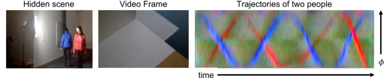
Hidden scene Video Frame
𝜙 time
Trajectories of two people
Figure 3-2: We show a result in which two people, one red and one black, walk around, illuminated by a large diffuse light, in an otherwise dark room. The resulting trajectories of their motion therefore show the colors of their clothing.
Our algorithm reconstructs a 1-D video of a hidden scene from behind an occluding edge, allowing users to track the motions of obscured, moving objects. In all results shown, the subject was not visible to an observer at the camera.
We present results using space-time images. These images contain curves that indicate the angular trajectories of moving people. All results, unless specified oth-erwise, were generated from standard, compressed video taken with a SLR camera.
3.4.1
Environments
We show several applications of our algorithm in various indoor and outdoor envi-ronments. For each environment, we show the reconstructions obtained when one or two people were moving in the hidden scene.
Indoor: In Fig. 3.4, we show a result obtained from a video recorded in a mostly dark room. A large diffuse light illuminated two hidden subjects wearing red and blue clothing. As the subjects walked around the room, their clothing reflected light, allowing us to reconstruct a 1-D video of colored trajectories. As correctly reflected in our constructed video, the subject in blue occludes the subject in red three times before the subject in red becomes the occluder. We note that our following results do not show the colors of the hidden people, and were taken in environments with more natural lighting.
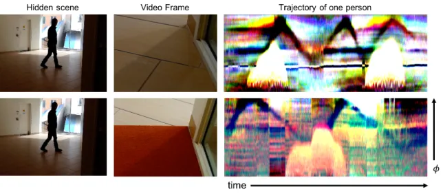
Figure 3-3: One-dimensional reconstructed videos of indoor, hidden scenes. Results are shown as space-time images for sequences where one or two people were walking behind the corner. In these reconstructions, the angular position of a person, as well as the number of people, can be clearly identified. Bright line artifacts are caused by additional shadows appearing on the penumbra.
Fig. 3-3 shows additional examples of 1-D videos recovered from indoor edge cameras. In these sequences, the environment was well-lit. The subjects occluded the bright ambient light, resulting in the reconstruction’s dark trajectory. Note that in all the reconstructions, it is possible to count the number of people in the hidden scene, and to recover important information such as their angular size and speed, and the characteristics of their motion.
Outdoor: In Fig. 3-4 we show the results of a number of videos taken at a com-mon outdoor location, but in different weather conditions. The top sequences were recorded during a sunny day, while the bottom two sequences were recorded while it was cloudy. Additionally, in the bottom sequence, raindrops appeared on the ground
during recording, while in the middle sequence the ground was fully saturated with water. Although the raindrops cause artifacts in the reconstructed space-time images, you can still discern the trajectory of people hidden behind the wall.
Figure 3-4: 1-D reconstructed videos of a common outdoor, hidden scene under various weather conditions. Results are shown as space-time images. The last row shows results from sequences taken while it was beginning to rain. Although artifacts appear due to the appearing raindrops, motion trajectories can be identified in all reconstructions.
3.4.2
Video Quality
In all experiments shown thus far we have used standard, compressed video captured using a SLR camera. However, video compression can create large, correlated noise that may affect our signal. We have explored the effect video quality has on results. To do this, we filmed a common scene using 3 different cameras: an iPhone 5s, a Sony Alpha 7s SLR, and a uncompressed RGB Point Grey. Fig. 3-5 shows the results of this experiment assuming different levels of i.i.d. noise. Each resulting 1-D image was reconstructed from a single frame. The cell phone camera’s compressed videos resulted in the noisiest reconstructions, but even those results still capture key features of the subject’s path.
Figure 3-5: The result of using different cameras on the reconstruction of the same sequence in an indoor setting. Three different 8-bit cameras (an iPhone 5s, a Sony Alpha 7s SLR, and an uncompressed RGB Point Grey) simultaneously recorded the carpeted floor. Each camera introduced a different level of per-pixel sensor noise. The estimated standard deviation of sensor noise, 𝜆, is shown in (B). We compare the quality of two sequences in (C) and (D). In (C), we have reconstructed a video from a sequence of a single person walking directly away from the corner from 2 to 16 feet at a 45 degree angle from the occluded wall. This experiment helps to illustrate how signal strength varies with distance from the corner. In (D), we have done a reconstruction of a single person walking in a random pattern.
3.4.3
Estimated Signal Strength
In all of our presented reconstructions we show images with an intensity range of 0.1. As these results were obtained from 8-bit videos, our target signal is less than 0.1% of the video’s original pixel intensities. To better understand the signal mea-surement requirements, we consider a simple model of the edge camera system that both explains experimental performance and enables the study of asymptotic limits. We provide a more detailed formulation in Appendix A.1.
We consider three sources of emitted or reflected light, show in Figure 3-6: a target cylinder (which acts as a rough model of a person), a hemisphere of ambient light (from the surrounding environment), and the occluding wall (which we assume to be much taller than the cylinder). We assume that all surfaces are Lambertian. The strength of the signal due to the cylinder, relative to the strength of the ambient illumination and light bouncing off the wall, can be computed using this model.
The observation plane can be split into three regions of interest, as shown the figure. Region 1 receives no light from the target cylinder. Region 2 receives increasing partial light from the cylinder as we move around the corner. Finally, region 3 sees
1 Scene 2 3
B
A
d
w
h
(x, y)Figure 3-6: Calculation of the contribution to the brightness of the target. Region 1 is the umbra region of the observation plane; none of the cylinder is visible from region 1, and thus its intensities do not change after introducing the target to the scene. Region 2 is the penumbra region; in region 2, part of the cylinder is visible. In region 3, the entire cylinder is visible.
the entire cylinder. We assume that all three regions receive equal contributions of light from the environment and the wall. We use this model to gain insight toward the contribution of the cylinder to the total brightness observed at each of these three regions on the observation plane.
The intensity in region 1 is simply 𝐼1 = 𝐴 + 𝐵. To determine the change of
intensity in region 3, we compute the difference between the reflected light with and without the cylinder. We can express the impact of the cylinder’s presence on a patch at a point (𝑥, 𝑦) in region 3 as follows:
𝐼3 = (𝐴 − 𝐵) 𝑤 𝑑 ∫︁ arctan(ℎ𝑑) 0 sin(𝜃)𝑑𝜃 (3.6) = (𝐴 − 𝐵)𝑤 𝑑 𝑑 √ ℎ2+ 𝑑2 (3.7)
where 𝑤, ℎ, and 𝑑 are defined as shown in Figure 3-6.
For region 2, the same calculation applies, but is additionally multiplied by the fraction of the cylinder that is visible from location (𝑥, 𝑦). More specifically, 𝛾1 to
be the angular boundary between region 1 and region 2 and 𝛾2 to be the angular
boundary between region 2 and 3. Then the brightness we observe at location (𝑥, 𝑦) in region 2 is given by
𝐼2(𝑥, 𝑦) =
tan−1(𝑦/𝑥) − 𝛾0
𝛾1− 𝛾0
𝐼3. (3.8)
For reasonable assumed brightnesses of the cylinder, hemisphere, and half-plane (150, 300, and 100, respectively, in arbitrary linear units), the brightness change on the observation plane due to the cylinder will be an extremum of -1.7 out of a background of 1070 units. This is commensurate with our experimental observations of ∼ 0.1% change of brightness over the penumbra region.
This model shows the asymptotic behavior of the edge camera. Namely, at large distances from the corner, brightness changes in the penumbra decrease faster than would otherwise be expected from a 1-D camera. This is because the arrival angle of the rays from a distant cylinder are close to grazing with the ground, lessening their influence on the penumbra. However, within 10 meters of the corner, such effects are small.
Chapter 4
Extensions of the Corner Camera
4.1
Reconstruction with a moving observer
The corner camera is a relevant contribution especially because wall corners are ubiq-uitous. Specifically, it could potentially be used in automotive collision avoidance systems. In order explore this possibility, we adapt the imaging system to detect motion behind the corner in real time, from a moving camera observer. This new problem setting introduces a few new challenges, which we begin to address in this chapter. First, the moving camera observer introduces deviations from the original light transport model, and complicates the recovery of the signal. Second, the system must be implemented efficiently to run in real-time. We address each of these prob-lems in the following sections, and offer insight to future directions to take to further this potential application.
4.1.1
Problems of a Moving Camera
The problem of stabilizing video from a moving camera has been extensively treated in vision and in robotics [10, 23, 28]. In this work, we make a few assumptions about the observed video frames. Namely, we assume that observer is moving slower than the frame rate of the camera, and will not encounter motion blur in the resulting video frames. Second, we assume that the corner of interest and its corresponding
observation plane is in every video frame we process. Moreover, we assume a compa-rable number of observed pixels from the moving camera observer to the stationary camera observer videos we process with the original formulation in Chapter 3.
The moving camera observer introduces two major problems when recovering our desired signal. First is the problem of video stabilization. Because the signal-to-noise ratio of the system is so low, the added noise from imprecise video stabilization adds artifacts to the recovered motion. Second is the changing viewing angle of the moving camera, which introduces unmodeled changes in the irradiance we observe from the ground.
Video Stabilization: Traditional methods of video stabilization involve detecting and matching features in consecutive frames, and calculating the perspective trans-form between the frames [10, 23, 28]. We approached this problem in the same way: we detected SIFT features in each frame, matched them using nearest-neighbor tech-niques, and used RANSAC to compute the homography between the frames. We also experimented with methods to track the distinctive wall corner and wall base structures, such as line segment detection and tracking. However, we found that the first approach was the least noisy and most reliable.
In Figure 4.1.1, we show results obtained on video that was stabilized using the classic feature detection and rectification approach. However, we note that homogra-phy estimation on smoother, less textured floors (such as the smooth tile floor at the top of the figure), is more error prone. As such, we notice large horizontal artifacts in the space-time images, due to misalignment with the background image. As a result, sharp features and large gradients in the background image interrupt and occasionally obscure the signal. This effect is especially noticeable against the small signal we try to recover.
Deviations from Light Transport Model Even if video alignment were perfect, the moving camera observer exacerbates certain deviations from our light transport model. In our original formulation of the corner camera, we can successfully
re-Figure 4-1: We show the reconstructed trajectories of the hidden scene, for a moving camera observer. We show results for two scenarios. In the top panel, the observation plane is a tiled surface; in the bottom, it is carpeted. The tile surface is more reflective, and shows noticeable changes in the brightness of the reconstruction as the camera viewing angle changes. The carpet shows a less dramatic effect. Horizontal line artifacts in both reconstructions are due to misalignment between the current frame and the mean frame.
cover our desired trajectories because the background irradiance was fairly constant throughout the input video. However, in the case of a moving camera, the viewing angle of the ground changes. For a non-Lambertian surface, such as reflective tile or wood, this causes our standard background subtraction to fail.
To address this problem, we subtracted an exponentially decaying moving aver-age frame from each input frame. In this way, we can approximately capture the most recent background irradiance. Despite this step, we still see shifts in color and brightness in the trajectories shown in Figure 4.1.1. Notice that for reflective tile, the changing viewing angle introduces dramatic brightness changes in the space-time images, while for a carpeted ground, the changes in brightness are weaker.
4.1.2
Real-time system
We implement the real-time interactive corner camera system in C++, using OpenCV [10]. In Figure 4.1.2, we show a screen shot of the system usage. The user can use either a
USB web camera or a PointGrey camera as a live input stream to the system; more work must be done to enable the system to process live video for other commercially available video recorders. The code and implementation are publicly available 1.
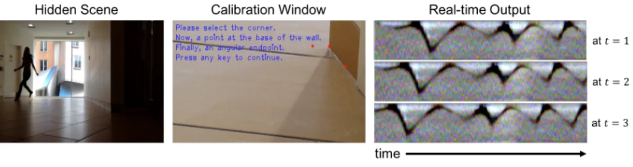
The user first selects the corner they are interested in, as well as the region at the base of the corner to observe (see Figure 4.1.2 middle). The system can then immediately begin processing the observations live. We show snapshots of real-time output at three different times in Figure 4.1.2.
Figure 4-2: Here we show an example of the usage of the real-time corner camera. In the left panel, we show the hidden scene of a girl behind a corner. In the middle panel, we show the interactive calibration window, in which the user selects the corner and observation region on the ground. In the right panel, we show snapshots of the real-time output at three different times. In each frame, we see a later part of the trajectory being added to the right of the space-time image.
For a stationary camera observer, the inference algorithm for recovering the hidden motion behind the corner is very lightweight. Once the light transport matrix A and resulting estimation gain matrix K is computed, the per-frame operation essentially becomes a matrix multiplication operation. Currently the system can process live video streams of frame rates up to 60fps.
We have begun adding video stabilization features to this system to allow for real-time moving video input, but this slows down our processing algorithm to only handle video streams with frame rates up to 25fps. Moreover, this system remains very sensitive, because of the remaining problems in extracting signal from a moving camera.
4.2
Stereo Tracking with Edge Cameras
In a hidden scene behind a doorway, the pair of vertical doorway edges yield a pair of corner cameras that inform us about the hidden scene. By treating the observation plane at the base of each edge as a camera, we can obtain stereo 1-D images that we can then use to triangulate the absolute position of a subject over time.
Figure 4-3: (A) The four edges of a doorway contain penumbras that can be used to reconstruct a 180∘ view of a hidden scene. Parallax occurs in the reconstructions from the left and right wall. (B) A hidden person will introduce an intensity change on the left and right wall penumbras at angles 𝜑(𝑡)𝐿 and 𝜑(𝑡)𝑅. We can recover the hidden person’s two-dimensional location using Eq. 4.2.
4.2.1
Recovering Depth with Adjacent Corner Cameras
A single corner camera allows us to reconstruct a 90∘ angular image of an occluded scene. We now consider a system composed of four edge cameras, such as an open doorway, as illustrated in Fig. 4-3(A). Each side of the doorway contains two adjacent edge cameras, whose reconstructions together create a 180∘ view of the hidden scene. The two sides of the doorway provide two views of the same hidden scene, but from different positions. This causes an offset in the projected angular position of the same person (see Fig. 4-3(B)). Our aim is to use this angular parallax to triangulate the location of a hidden person over time. Assume we are observing the base of a doorway, with walls of width 𝑤 separated by a distance 𝐵. A hidden person will introduce an intensity change on the left and right wall penumbras at angles of 𝜑(𝑡)𝐿 and 𝜑(𝑡)𝑅 , respectively. From this correspondence, we can triangulate their 2-D location.
Figure 4-4: The four edges of a doorway contain penumbras that can be used to reconstruct a 180∘ view of a hidden scene. The top diagram indicates the penumbras and the corresponding region they describe. Parallax occurs in the reconstructions from the left and right wall. This can be seen in the bottom reconstruction of two people hidden behind a doorway. Numbers/colors indicate the penumbras used for each 90∘ space-time image.
𝑃𝑧(𝑡) = 𝐵 − 𝜂 (𝑡) cot 𝜑(𝑡)𝐿 + cot 𝜑(𝑡)𝑅 (4.1) 𝑃𝑥(𝑡) = 𝑃𝑧(𝑡)cot 𝜑(𝑡)𝐿 (4.2) 𝜂(𝑡) = ⎧ ⎪ ⎪ ⎪ ⎪ ⎪ ⎨ ⎪ ⎪ ⎪ ⎪ ⎪ ⎩ 𝑤 cot(𝜑𝑅) 𝑃𝑥 ≤ 0 0 0 ≤ 𝑃𝑥 ≤ 𝐵 𝑤 cot(𝜑𝐿) 𝑃𝑥 ≥ 𝐵 (4.3)
where (𝑃𝑥, 𝑃𝑧) are the 𝑥- and 𝑧-coordinate of the person. We define the top corner
of the left doorway, corner 1 in Fig. 4-3(A), as (𝑃𝑥, 𝑃𝑧) = (0, 0).
Assuming the wall is sufficiently thin compared to the depth of moving objects in the hidden scene, the 𝜂(𝑡) term can be ignored. In this case the relative position
of the doorway (e.g. 𝐵 or 𝑤). In all results shown in this paper, we have made this assumption.
While automatic contour tracing methods exist [12], for simplicity, in our stereo results, we identify the trajectories of objects in the hidden scene manually by tracing a path on the reconstructed space-time images.
4.2.2
Experiments and Results
Figure 4-5: We performed controlled experiments to explore our method to infer depth from stereo edge cameras. A monitor displaying a moving green line was placed behind an artificial doorway (A) at four locations: 23, 40, 60, and 84 cm, respectively. (B) shows reconstructions done of the edge cameras for the left and right wall when the monitor was placed at 23 and 84 cm. Using tracks obtained from these reconstructions, the 2-D position of the green line in each sequence was estimated over time (C). The inferred position is plotted with empirically computed error ellipses (indicating one standard deviation of noise).
We show that this method can estimate the 2D position of a hidden object using four edge cameras, such as in a doorway. We present a series of experiments in both controlled and uncontrolled settings.
Controlled Environment: We first conducted a controlled experiment in which a monitor displaying a slowly moving green line was placed behind two walls, separated
Figure 4-6: The results of our stereo experiments in a natural setting. A single person walked in a roughly circular pattern behind a doorway. The 2-D inferred locations over time are shown as a line from blue to red. Error bars indicating one standard deviation of error have been drawn around a subset of estimates. Our inferred depths capture the hidden subject’s cyclic motion, but are currently subject to large error. by a baseline of 20 cm, at a distance of roughly 23, 40, 60, and 84 cm. Fig. 4-5B shows sample space-time reconstructions of each 180∘ edge camera. The depth of the green line was then estimated from trajectories obtained from these space-time images. Empirically estimated error ellipses are shown in red for a subset of the depth estimates.
Natural Environment: Fig. 4-6 shows the results of estimating 2-D positions from doorways in natural environments. The hidden scene consists of a single person walking in a circular pattern behind the doorway. Although our reconstructions capture the cyclic nature of the subject’s movements, they are sensitive to error in the estimated trajectories. Ellipses indicating empirically estimated error have been drawn around a subset of the points.
We note that there are multiple sources of error that can introduce biases into location estimates. Namely, because 𝑃𝑧 scales inversely with 𝑐𝑜𝑡(𝜑𝐿) + 𝑐𝑜𝑡(𝜑𝑅), small
errors in the estimated projected angles of the person in the left and right may cause large errors in the estimated position of the hidden person, particularly at larger depths. Misidentifying the corner of each occluding edge will also introduce systematic error to the estimated 2-D position.
To better understand how to mitigate these sources of error, we propose to conduct more controlled experiments, in the spirit of the controlled monitor experiment, to understand when and how our method breaks down.
We also propose to directly model the doorway system, as a way to recover two-dimensional information. The depth and angular location are encoded in the geometry of the doorway, and by directly modeling this, we may be able to more precisely reconstruct two-dimensional location. In Chapter 5, we explore ways to model and reconstruct two dimensional scenes in a similar way.
Chapter 5
Reconstructing in Two Dimensions
Because of their ubiquity, we have thus far focused on wall edges and corners as occluders in naturally-occurring camera systems. However, the vertical edge can only integrate light from the hidden scene in vertical slices; all of the light in a single vertical slice is squashed together in our observation. As such our reconstructions of what happens behind a corner are in one spatial dimension. In this chapter, we expand our scope of accidental camera systems to recover 2D projections of a hidden scene.
In Section 5.1, we develop the imaging model for a spherical occluder. We find that because of the geometry of the occluder, reconstructed pixels are warped and ambiguous. In Section 5.2, we explore rectangular occluders, which suffer less from this ambiguity. Because of the sharp corners of rectangles, adjacent pixels at the edges can more clearly reconstructed than for the spherical occluder.
5.1
Spherical Occluders
Spheres are also commonly occurring, in doorknobs and balls, and are not constrained to recover scenes in a single dimension. In Figure 5.1, we show a schematic of the imaging system created by a sphere placed on the floor. We show in 5.1(A) a sphere in between the wall and two cylinders. The wall is our observation plane, upon which we can observe the faint shadow cast by the sphere. The camera sees observation
plane behind the sphere, but cannot see the two cylinders. We project the hidden scene onto an imagined 2D plane, shown in Figure 5.1(B). We place this plane at a depth of our choosing.
Figure 5-1: We show a schematic of an imaging setup used for the spherical occluder. In (A), we show a sphere in between the observation plane and two colored cylinders. The camera can see the observation plane, but the two cylinders are out of sight. In (B) we show the discrete parameterization of the light from the hidden scene. We choose a grid parallel to the observation plane, placed at a known depth. The 𝑖-th column of the transport matrix will be the observed shadow from a point source placed at the 𝑖-th location on this grid.
We use this imagined 2D plane to model the light from the hidden scene as imag-ined light sources on this plane, 𝐿ℎ(𝑥, 𝑦). We assume a discretized image of 𝑁 = 𝑅×𝐶
evenly spaced point sources on this plane for reconstruction. While we could take the approach of 3.1 and linearly interpolate between sources to better approximate a continuous 𝐿ℎ(𝑥, 𝑦), we take this approach for simplicity.
With this parameterization, we can easily derive the linear relation between the 𝑀 observed pixels y and the 𝑁 hidden scene parameters x. In Figure 5.1(B), we show an impulse response for the 𝑖-th point source of x; as before, this rasterized response forms the 𝑖-th column of A. Each column 𝑖 of the transport matrix A is the observed response of the ground irradiance to an isotropic light placed at the 𝑖-th element of x, at the corresponding angle 𝜃𝑖. We show in Figure 5.1(B) an example of a column
of our transfer matrix imposed on a picture of an experimental observation. The reshaped column we show is the impulse response of the middle pixel in our scene.
Figure 5-2: (A) An image of the observation plane behind a sphere and scene. The sphere creates a shadow on the observation plane that contains information about the scene behind it. (B) The response of the system to a single point light source in the middle of our scene. These impulse responses form the columns of our transfer matrix A. (C) The estimation gain image of middle pixel in our scene. Namely, the 𝑖-th estimation gain image shows what information in the observation is used to reconstruct the 𝑖-th pixel in the scene.
5.1.1
Inference
In this work, we recover 2D static images, but this method can easily be extended to videos to recover motion.
Likelihood: We relate the observed 𝑀 -pixels on the projection plane, y, to the 2D projection of the hidden scene, 𝐿ℎ(𝑥, 𝑦), which we discretely approximate with a
rasterized grid of 𝑁 = 𝑅 × 𝐶 terms, x. Assuming i.i.d. Gaussian noise, the relation between y(𝑡) and x(𝑡) can be written as
y(𝑡) = 𝐿𝑣 + Ax + w, w ∼ 𝒩 (0, 𝜆I), (5.1)
where 𝐿𝑣 is the unmodeled light from the visible scene.
Again, defining ̃︀A be the column augmented matrix [1 A], we can express the likelihood of an observation given x and 𝐿𝑣 as:
𝑝(y|x, 𝐿𝑣) = 𝒩 (︁ ̃︀ A[︀𝐿𝑣 x𝑇 ]︀𝑇 , 𝜆I )︁ . (5.2)
Prior: We enforce spatial smoothness in both dimensions of the hidden image x. That is, we again use an L2 smoothness regularization over the gradients in 𝑥 and
𝑦. We define the 𝑅𝐶 × 𝑅𝐶 matrix Gx
R,C as the operator returning the horizontal
gradients of the rasterized 𝑅 × 𝐶 image. We define GyR,C similarly. Then, our prior can be expressed as 𝑝(x) = 𝒩 (︂ 0, 𝜎2(︁GxR,C𝑇GR,Cx + GyR,C𝑇GyR,C)︁ −1)︂ .
As before, we note that the visible light 𝐿𝑣 has an under-determined relationship
with the light on the observation plane and encode this in the posterior below.
Posterior: By combining the defined Gaussian likelihood and prior distributions, we obtain a Gaussian posterior distribution of x and 𝐿𝑣,
𝑝(x, 𝐿𝑣|y) = 𝒩 (︂ [︁ ˆ𝐿𝑣 ˆx𝑇]︁𝑇 , Σ )︂ Σ = ⎡ ⎣𝜆−1Ã︀𝑇A + 𝜎̃︀ −2 ⎛ ⎝ 0 0 0 GxR,C𝑇GxR,C ⎞ ⎠+ 𝜎−2 ⎛ ⎝ 0 0 0 GyR,C𝑇GyR,C ⎞ ⎠ ⎤ ⎦ −1 [︁ ˆ𝐿𝑣 xˆ𝑇]︁𝑇 = Ky = 𝜆−1Σ ̃︀A𝑇y (5.3)
where the maximum a posteriori estimate is given by ˆx.
We show the operation we perform on y to recover an element 𝑖 of x, in Fig-ure 5.1(C). This is one row of the estimation gain matrix, K, visualized to show the pixel-wise contributions of y to the estimated 𝑥𝑖. We see that for this
geome-try, we perform a derivative across the edge of the 𝑖-th impulse response shown in Figure 5.1(B).
5.1.2
Experimental Results
We test our method with two experimental setups. In the first, shown in Fig-ure 5.1.2(A), we project a hidden scene from a monitor toward a white wall, four feet away. A standard 9 inch soccer ball sits halfway between the monitor and ob-served wall. The scene is not visible from the camera. The room contains other
Figure 5-3: We show results for our first experimental scenario. In (A), we show the setup: we project the hidden scene from a monitor onto a blank observation wall, four feet away. A 9 inch soccer ball sits halfway between the two. In (B), we show the hidden scenes we project from the monitor, and in (C), we show the resulting reconstructions.
objects, as well as ambient lighting.
For our reconstructions, we place our 2D projection plane directly at the location of the monitor, four feet away from the wall. Using these location measurements, we then analytically compute the transport matrix A. We note that this method of obtaining A is error-prone, which creates artifacts in the reconstructions.
We then project the simple scenes in 5.1.2(B) from the monitor, and obtain the static 2D reconstructions shown in Figure 5.1.2(C). We note that our method causes some artifacts, resulting from several sources of error. The first is from the error in the measurements we use to construct A. This error can be combated with a more precise calibration method, which involves capturing each impulse response for the 2D projected grid we wish to reconstruct. We develop and employ this calibration method to reconstruct 4D light fields in Chapter 6.
In our second setup, shown in Figure 5.1.2, we reconstruct two simple objects made of paper, 1 foot tall, illuminated by a large diffuse light. All else remains the same; we continue reconstructing the 2D projection four feet away from the wall, we keep the soccer ball halfway between the two planes, and the room contains ambient