HAL Id: halshs-01149595
https://halshs.archives-ouvertes.fr/halshs-01149595
Submitted on 7 May 2015
HAL is a multi-disciplinary open access
archive for the deposit and dissemination of sci-entific research documents, whether they are pub-lished or not. The documents may come from teaching and research institutions in France or abroad, or from public or private research centers.
L’archive ouverte pluridisciplinaire HAL, est destinée au dépôt et à la diffusion de documents scientifiques de niveau recherche, publiés ou non, émanant des établissements d’enseignement et de recherche français ou étrangers, des laboratoires publics ou privés.
The Size of Informal Economy and Demand Elasticity
Estimates Using Full Price Approach: A Case Study for
Turkey
Armagan Tuna Aktuna-Gunes, François Gardes, Christophe Starzec
To cite this version:
Armagan Tuna Aktuna-Gunes, François Gardes, Christophe Starzec. The Size of Informal Economy and Demand Elasticity Estimates Using Full Price Approach: A Case Study for Turkey. 2014. �halshs-01149595�
Documents de Travail du
Centre d’Economie de la Sorbonne
The Size of Informal Economy and Demand Elasticity Estimates Using Full Price Approach:
A Case Study for Turkey
Armagan Tuna AKTUNA-GUNES, François GARDES,
Christophe STARZEC
The Size of Informal Economy and Demand Elasticity Estimates Using Full
Price Approach: A Case Study for Turkey
Armagan T. Aktuna-Gunes* François Gardes** Christophe Starzec*** December 12, 2014
________________________
* Paris School of Economics, Université Paris I Panthéon-Sorbonne, Centre d’Economie de la Sorbonne, 106-112 Boulevard de l’Hôpital, 75647, Paris Cedex 13, France ; courriél : Armagan.Aktuna-Gunes@univ-paris1.fr
** Paris School of Economics, Université, Paris I Panthéon-Sorbonne. Courriél : paris1.fr
Abstract
In this article, the size of informal economy is measured by using the full price method proposed by Gardes F. (2014). As an extension of this method, price elasticities are re-estimated by integrating the underreported earning shares both for wage workers and self-employers from cross-sectional data covering 2003–2006 in Turkey. The contribution of this paper is threefold: The size of informal economy is estimated by a statistical matching of the Turkish Family Budget and Time Use surveys through a complete demand system including full prices. Second, more accurate price and income elasticities are estimated by using the monetary incomes from informal activities for an emerging economy such as Turkey. Third, extended full price estimation of demand elasticities allow us to discover for which consumption group households are more likely to engage in informal work.
Keywords: informal economy, complete demand system, full prices, demand elasticity JEL Classification: E26, D1, D12, J22
Résumé
Dans cet article, la taille de l’économie informelle est estimée en utilisant la méthode du prix complet proposée par Gardes F. (2014). Les élasticités de prix sont estimées en intégrant les parties sous-déclarés des revenus des travailleurs indépendants et salariés en utilisant des données transversales couvrant 2003-2006 en Turquie. La contribution de cet article est triple: La taille de l'économie informelle est estimée par l’appariement statistique des enquêtes turques sur le Budget des Familles avec l’enquête sur l’Emploi du Temps en intégrant les prix complets dans le système complet de demande. Deuxièmement, les élasticités des prix et de revenu sont estimées plus justement en élargissant les ressources monétaires avec les parts des revenus provenant des activités informelles, pour une économie émergente comme la Turquie. Troisièmement, cette dernière nous permet de découvrir pour quels groupes de consommation sont les ménages plus susceptibles de s’engager dans le travail informel.
Mots-clés : économie informelle, système complet de demande, prix complets, élasticités
de demande
Introduction
The common thought is that price elasticities estimates in macroeconomic time-series suffer from aggregation biases and microeconomic information problems due to socio-economic characteristics of the population. These estimates may depend on the various sources of income shares gathered from formal and informal activities. For instance, price elasticity estimations may suffer from the biases due to group heterogeneity which may arise because the social classes may not participate in the same manner in informal and domestic activities. Furthermore, each household may decide to use different income sources with as a consequence different propensities to buy luxuries from self-employment income or necessary goods from regular wage income1.
Our aim in this paper is to identify how earnings from informal activities affect the estimated values of price elasticities. For this purpose, we use the full price model framework proposed by Gardes (2014). The advantage of this model is that the problem of lack of prices data in households surveys is eliminated which allows to estimate full income and full price elasticities. In this respect, the importance of this paper is to consider the domestic activities together with informal ones both for wage earners and independent workers. It helps to measure the full cost of their consumption which allows obtaining more adequate price elasticities especially for emerging economies.
The structure of paper is as follows: Section 1 presents the construction of full price method and specifies informal economy estimation model using full prices based on the demand approach extended to informal sector activities. Section 2 describes our sample and provides descriptive statistics for Turkey from the Household Budget Surveys between 2003 and 2006 and Time Use Surveys for 2006. Section 3 reports the results. Section 4 offers concluding remarks.
1. Model
1.1. The Full Price Concept
The Full price method based on Becker’s model of the allocation of time (1965). Full
prices incorporate either shadow prices linked to constraints faced by the agent, or shadow prices corresponding to non-monetary resources such as time (see Gardes et al., 2005). The idea in this method is to represent them by the ratio of full expenditures over the monetary, thus suppressing the quantity consumed (see Gardes, 2014).
Definition
The full prices are the set of ratios separately computed for each consumption group represented in consumer budget as a share. The canonical definition of full price is the ratio of full expenditure over the monetary expenditure for any given expenditure bundle. Full
1
This is “the bias from confusing preference heterogeneity with under-reporting effects […]” (see Lyssiotou et al., 2004) that also can arise.
expenditure part of full price is consists of two parts: first,p x as monetary expenditure i i
defined upon the monetary price pi and consumption quantity of xi for the market goods i. The second part consists of the time cost value wt as a product of time spend ti i for the consumption activity i and the market wage rate w. The full expenditure could be defined as (piwtih)xih depending on households’ characteristics by means of its time participation to activity i: t and market wageih w . Thus the full prices for the activity i is measured by h
( ) 1 ih i h ih h ih ih i ih i x p w w p x p (1)
The denominator and the nominator in equation (1) respectively are monetary expenditures and full expenditure (i.e. monetary expenditures and monetary time values of domestic activities combined) respectively. Thus, the right side of the equation reveals that full prices no longer depend on consumption quantities. Therefore, the information regarding full price only obtained through wage rates and time spent. The market wage rate refers to
sole market substitution and nothing more than hourly minimum wage rate. In order to avoid
any possible endogeneity problems during the estimation of elasticities using the full demand equation, full expenditures could also be computed by the opportunity cost (potential earnings) method.
1.2. The Demand System
Elasticities in demand could be estimated for extended expenditures using full price specification given in the equation (1). We choose the Linearize Almost Ideal Demand System (LA-AIDS) sample regression function to estimate elasticities for each consumption group including using extended full prices. This system based on Almost Ideal Demand System (AIDS) specification proposed by Deaton and Muellbauer (1980), one of the most common nonlinear models used to estimate demand elasticities. The advantage of this model is that the estimation could easily be approximated to its linear form2. Pashardes (1993) treated the estimation bias of price coefficients by considering as an omitted variable problem due to use of the Stone price index in the model specification. To overcome this endogeneity problem, Pashardes (1993) proposed to approximate formulas of price parameters.
In our estimation, an integral demand function should exist; hence, utility maximization or cost minimization determine the expenditure level. The Linearize Almost Ideal Demand System (LA-AIDS) sample regression function is estimated under homogeneity, symmetry and additivity constraints for each consumption group including extended full prices.
1 log log n i i i ij j i i j x w Z m
(2) 2For ith of n commodity groupw , x, m, and Z respectively represent budget share,
household expenditure, corrected Stone’s price index (by Pashardes, 1993) formulas), full prices for each commodity groups, socio-economic characteristics respectively.
1.3. Demand System Specification of Informal Economy Using Full Prices
Implementing the estimation of the demand system has become a challenge since there are almost no reliable sources of local price data and even when such data exist it is very likely to be incomplete for all commodities other than food3. Therefore, there could only be three reasons for ignoring the changes in relative prices while estimating the size of informal economy in developed economies, using the demand system approach (Fortin et al. 2009). First, there are no price indices at the regional level in the Household Budget survey data. Second, in general, the period of analysis is relatively short; hence, it considers the average increase in prices by deflating income by an index of consumer prices assumed to be enough for the estimation. Furthermore, the model allows that the constant Engel curves vary from one year to the next. As a matter of fact, these could not be assumed as reasonable with regards to developing economies. High level inflation rates and regional differences in relative prices for the same groups of goods and services create the need to consider relative prices in the complete demand system approach of measuring the size of informal economy.
In this sense, We use the demand system approach to estimate the size of the informal economy in Turkey following the methodology based on the analysis of the household consumption behavior proposed by Pissarides and Weber (1989), Lyssiotou et al. (2004), Fortin et al. (2009) and Aktuna-Gunes et al. (2014). We suppose that only the sources other than self-employment and wage incomes have been perfectly reported since the tax is deduced. Thus, self-employment income and wage worker incomes can be under reported. It allows us to identify the coefficients of the under reporting due to these incomes by assuming that the consumption of each good, related to its marginal propensity of consumption, is the same as in the case of the revenue actually observed. More systemically, let true income (Y*) be separated into three sources denoted a, s, r which respectively correspond to other income sources, wages and self-employment income. The proportions of wage and self- employment incomes vary a lot between 2003 and 2006 as indicated in table 1:
Table 1: Income shares of self employers and wage-earners between 2003 and 2006 (% of
GDP)
2003 2004 2005 2006
Self Employed 25.09 26.56 25.88 21.37 Wage Earners 50.70 54.50 57.00 58.90
Source: Turkish Statistical Institute (TURKSTAT)
3
Elasticities in demand are estimated from macro time-series is in general considered as being not robust to the specification of the demand system and they give no information on the change of price and income effects according to household characteristics. A macro time-series using estimation has the usual problems that result from co-linearity between relative price changes, aggregation biases whenever individual agents face different prices changes or have different preferences.
The total reported (true) income is supposed to be a weighted sum of these three sources: (3) This equation implies that the true income must be equal to the sum of the observed income (Ya, Ys, Yr) multiplied by their corresponding factor (θa, θs, θr), where we suppose θm ≥ 1 (i.e.,
under reporting) and θa = 1 (correct observation of the other incomes). Such hypothesis allows
us to estimate the under reporting part of self-employers and wage workers4 under the assumption that they may also save certain parts of their under reported income to finance durable and non-durable goods purchases. It allows us to calculate the size of the underground economy and the saving tendencies with respect to the under reporting part of declared incomes by an estimation of θr and θs. In order to impose the constraint on the θr and θs
parameter (θr,s ≥ 1), Fortin et. al (2009) propose to express it by (1+ek) where k is a parameter
estimated by the model. Additionally, we suppose that the true value of self-employment and wage income (Yr* and Ys*) can respectively be then denoted as (1+ek)*Yr and (1+el)*Ys
where l represents the parameter as an under reported part estimated for wage workers.
Finally, we could determine the sum of each source of income as a ratio of the reported total income: ym = Ym/Y, where Y is the sum of other sources as fees, government transfers,
etc. as well as wages and self-employment incomes. Following the model proposed by Aktuna-Gunes A. et al. (2014), we consider all goods and services with full price values in the estimation model as follows:
, 1 , , , , 3 2 ( ) ln Y ln( ) ln Y ln( ) log n ih i ij jh in r s i h m m j n m a s r i h m m i ih ih m a s r Z y y y e w (4)
where w, , Z, j and i represent respectively the budget share the full prices and the
household characteristics vector (which allows us to take into account the heterogeneity of preferences). We cannot expect that the individuals from different social groups have the same reaction in consumption and saving choices with respect to the different types of incomes especially when there is uncertainty about these revenues. In accordance with Lyssiotou et al. (2004), we thus introduce in each equation linearly the powers of incomes r and s (∑3n=1 λin(yr,s)n ) in order to reflect the relative importance of self-employed and wage incomes in the total household’s income. The purpose of this expression is to diminish any possible confusion between consumption heterogeneity and the phenomenon of the under-reported part of self-employed and wage earners' income.
4
This is a necessary constraint. According to the research conducted by Republic of Turkey Social Security Institution in 2011, 75 of every 100 wage workers, declared as minimum wage, is lower than their real wage rate. Therefore, the part of the disposable income of regular employee represents 42.8%, 54.5%, 57%, 58.9% in total GDP respectively for the years between 2003–2006
* , , Yh mYmh m a s r
1.4. Full Prices with Informal Earnings
In order to better show the impact of undeclared incomes on consumption decision, we propose to integrate informal earnings into income and use full prices to obtain more robust elasticities especially for developing economies as Turkey. We suppose that the decomposition defined in equation 3 applies for total expenditure X as far as wage earners and self-employed are concerned:
* , m m m m s r X X
(5)We can rewrite the full price in the equation (1) for the activity i by the ratio full expenditures over their monetary component including undeclared income parts as follows
* ( ) 1 ih m i h ih h ih ih m i ih m i x p w w p x p (6) * ih
is the corrected full prices (i.e. also full prices extended by informal earnings)
computed by multiplying the monetary expenditures by under-reported parameters. Time use values need not be corrected because, it is supposed that time values are truly declared.
1.5. Demand Elasticities
Income Elasticity
We suppose that two separate optimizations exist for monetary and for time allocation. In this case the budget shares for full expenditure could not be computed as the average of their respective shares due to the nonlinearity of demand functions.
With wim, wit, wis respectively monetary , time and full budget shares for commodity i, the full income elasticity Eif can be calculated in terms of estimated monetary and time elasticities: 1 1 1 1 im it if im it if if w w E E E w k w k (7)
Where k is the derivative of the temporal income over the monetary income.
The second problem is the quality effects which exist in full price and expenditure data. Indeed, an increase (in the cross-section dimension i.e. between two households) of the full price for each commodity may result either from the difference (between the two agents) of the opportunity cost w or from the difference of their time allocated to activity i. Both causes may increase the quality of this activity, by means of an increased productivity (which can be supposed to be positively related to w) or of the time devoted to i. In our matched dataset, we correct this endogenous quality by supposing that local prices are replaced by the individual full prices for each household following the correction technique proposed by Cox and
Wohlgenant(1986). Thus, we adjust the full prices for each commodity group by adding the value of constant to the residual of the regression based on the unit values on selected socio-demographic variables, such as household income, region, household size.
Price Elasticity
Price elasticities could be calculated in the same manner as calculated by the AIDS model by means of price coefficients and of demand system parameters as follows:
/ ˆ i j ij x j ij i E w w (8)
Where is the Kronecker index. Therefore, following the method proposed by De Vany ij
(1974), full price elasticities would be directly calculated by summing up Hicksian monetary and time elasticities respective to their shares. In which the monetary price and time elasticities correspond respectively to
/ / i j i j j j x p x i j p x E E x (9i) / / i j i j j j x t x i j wt x E E x (9ii) 2. Dataset
We use two household surveys: the Time Use Survey (TUS) and the Household Budget Surveys (HBS) from Turkish Statistical Institute (TURKSTAT). The Household Budget Surveys have been conducted on a total of 2 160 monthly and 25 920 annually sample households in 2003 and on a total of 720 monthly and 8 640 annually sample households in 2004, 2005 and 2006. In the 2006 Time Use Survey, approximately 390 households were selected each month giving a total of 5070 households over the whole year. Within these households 11 815 members aged 15 years and over were interviewed and were asked to complete two diaries – one for a weekday and one for a day on the weekend – recording all of their daily activities within 24 hours at ten-minute intervals. This 2006 Time Use Survey is matched independently by the four Family Budget Surveys realizing a repeated cross-section of monetary and time expenditure data.
2.1. Statistical Matching and Valuation of Time
We combine the monetary and time expenditures into a unique consumption activity at the individual level. We proceed with the matching of these surveys by regression on similar exogenous characteristics in both datasets as age, matrimonial situation, possession of cell phone, home ownership, number of household members, geographical location separately for head of household and wife5.
5
More precisely, we estimate 8 types of time use at Time Use Survey (TUS) which are also compatible with the available data from Household Budget Survey (HBS) as follows:
Food Time (TUS) with Food Expenditures (HBS)
Personal Care and Health Time (TUS) with Personal Care and Health Expenditures (HBS) Housing Time (TUS) with Housing Expenses (HBS)
Clothing Time (TUS) with Clothing Expenditures (HBS) Education Time (TUS) with Education Expenditures (HBS) Transport Time (TUS) with Transport Expenditures (HBS) Leisure Time (TUS) with Leisure Expenditures (HBS) Other Time (TUS) with Other Expenditures (HBS)
The food Time consists only of cooking because it is not possible to separate eating activity from Personal Care in the time use survey. Care time consists of personal care, commercial-managerial-personal services, helping sick or old household person and eating activity. Housing Time corresponds to household-family care as home care, gardening and pet animal care, replacement of house-constructional work, repairing and administration of household. Clothing Time consists of washing clothes and ironing. Education Time includes study (education) and childcare. Transport Time consists of travel and unspecified time use. Leisure Time corresponds to voluntary work and meetings, social life and entertainment such as culture, resting during holiday, sport activities, hunting, fishing, hobbies and games, mass media like reading, TV/Video, radio and music. Other Time includes employment and labor searching times.
Valuation of time
Given that individuals spend their time in the production of goods and services and that time has a cost, we consider the full expenditure of households as the sum of their monetary expenditure plus the cost of time; with the cost of time spent on domestic activities being no more than the value that it would have in the labor market. Therefore, in this study, by taking advantage of having TUS and HBS data, we choose the opportunity cost method. Two possible opportunity cost methods for the valuation of time spent on domestic activities can be used: First method dictates that we impute the wages net of taxes for non-working individuals using the two-step Heckman procedure: supposing that only time use is perfectly exchangeable for non-market and market activities. In that method the first step estimates a probit equation for participation. The natural logarithm of monthly income, age, age-squared, education dummies, urban variables with the explanatory variables of couples, number of children, number of household members are used for predicting the underlying wage rate of households that do not work. Thus, in the second stage the opportunity cost of non-market work is estimated as the expected hourly wage rate in the labor market for those men and women not working. Second method refers to sole market substitution which consists of
imputing the same hourly rate for all individuals represented in the surveys, namely minimum wage rate for Turkey in 2003, 2004, 2005 and 2006. Therefore, in this paper, the monetary values of time expenditures parts are calculated using the minimum wages for each year deflated on the base year 2003. The opportunity cost may rather be between these two values. (see the discussion in Gardes, Starzec, 2014). The purpose of this double recovery is to compare results and to test the robustness of the chosen valuation method.
3. Empirical Results
Informal Economy with Full Prices
We estimate a complete demand expenditure system in equation (4) by integrating full prices, using the Generalized Method of Moments (GMM) for monetary and full expenditure (monetary time values of domestic activities added monetary expenditures) respectively. The estimation of the model for full expenditure and exclusive monetary expenditure from the pooled cross-sectional data covering the period of investigation 2003-2006, for self-employed and wage earners are presented in Tables 6-9.6 Only the parameters estimates of the seven budget share equations are reported in these tables, since the parameters of the eighth equation (other goods/services) are redundant due to the adding up condition. The test for the instrumentation of the endogenous variable of income shows that the used instruments are not weak. Specifically, the Stock-Yogo test with the bias method rejects the hypothesis of the presence of weak instruments7.
The size of informal economy for different types of incomes (self-employment, wages) both for monetary and full expenditure approaches is computed by scaling up the under-reporting parameters k and v with share of self employers and wage-earners' income that contributes to the GDP. The results are presented in Table 2.
Table 2: The Size of Informal Economy with Full Prices for the Years between 2003 and
2006 (In %)
6
For the detail of proposed instruments see Table 10 on Appendix I.
7
F-statistic of the first stage (15.36) is higher than the critical value of 10% of the maximal instrumental variable bias (11.49). For the estimation results see Table 6.
Year Parameters k, v
(Std. Err) 2003 2004 2005 2006 Average
Size of informal economy for monetary exp enditure estimation (SE)ᵃ 1.58 *** (0.316) 39,64% 41,96% 40,89% 33,76% 39,07% Size of informal economy for monetary exp enditure estimation (WE)ᵇ 0.48**
(0.149) 24,34% 26,16% 27,36% 28,27% 26,53%
Size of informal economy for full exp enditure estimation (SE)ᵃ 1.91 **
(0.852) 47,92% 50,73% 49,43% 40,82% 47,22%
Size of informal economy for full exp enditure estimation (WE)ᵇ 0.58*** (0.248) 29,41% 31,61% 33,06% 34,16% 32,06% ***p <0.01, **p<0.05, *p<0.1
The corresponding size of informal economy for the monetary expenditure approach and based on self-employed under-reporting decreases in the period considered (2003-2006) from 39.64% to 33.76%. The full expenditure approach yields larger shares from 47.92% to 40.82% of GDP in the same period. The under-reporting in incomes from wages rises from 24.34% to 28.27% between 2003 and 2006 for the monetary expenditure approach and from 29.41% to 34.16% for the full expenditure approach. Both estimations of informal economy using full and monetary expenditures are around two third of the GDP, slightly higher in 2004-2005 when compared to 2003 et 2006.We take into account that domestic activity leads to a significant increase in the under reporting-income ratio and thus in the size of the informal sector (around +20%) both for self-employers and wage-earners. The change in this size, observed in 2006, is due to the decrease of the part in income of independent workers and the increase of the part of wage-earners’ income in GDP: by 14.4% and 16.1% respectively.
Demand Elasticities
Elasticity results are obtained by regrouped time activities and monetary expenditures in eight different commodities for Turkey. The elasticities are calculated on the base of full prices. One of the goals of this paper is to provide consistent parameters estimates reflecting the consumption behavior since informality exists. However, certain aggregate goods such as “education” may have a higher monetary expenditure and time intensive due to number of children living with family, than a couple of seniors. Such problems should disappear by correcting the full prices by integrating informal earnings. The contribution of this identification of demand elasticities by informal earnings is that gives us an idea surrounding household engagement in informal activity sensitivities. In other words, it allows us to discover for which consumption group households are more likely to engage in informal work.
For the present analysis, we have decided to show the results for the whole sample for all the commodity groups. The first three columns of Tables 3-4 represent standard monetary, time and full income elasticities while the last three ones underneath illustrate the impact of the informality on the results. Table 3 shows income elasticities for eight consumption groups with corrected variance for each. Most of its goods have an unitary demand. An increase (decrease) in income generates a proportional increase (decrease) of demand for goods. Extended monetary results regarding to not-extended monetary ones indicates that only food, housing are necessary. Therefore, once the domestic activities are included in to the estimation, full elasticity results imply more inelastic demand for food, personal care with health, leisure in Turkey. It is worth noticing that at the population level food is a necessary good, as expected from theory, and leisure is mostly a luxury good.
Table 3: Income Elasticities (Standard Errors in Parenthesis)* Whole Population 0,866 (0,0163) 0,774 (0,0011) 0,938 (0,0201) 0,815 (0,0293) 0,729 (0,0039) 0,884 (0,0238) 0,971 (0,0111) 0,826 (0,0090) 1,064 (0,0071) 0,910 (0,0192) 0,796 (0,0019) 1,001 (0,0181) 1,123 (0,0134) 0,977 (0,0026) 0,961 (0,0104) 1,208 (0,0125) 0,982 (0,0030) 0,983 (0,0104) 1,285 (0,0215) 0,735 (0,0010) 1,312 (0,0084) 1,211 (0,1873) 0,671 (0,0176) 1,233 (0,1547) 1,034 (0,0085) 0,984 (0,0104) 1,045 (0,0039) 1,357 (0,0319) 1,152 (0,0242) 1,306 (0,0403) 1,296 (0,0176) 1,053 (0,0083) 1,163 (0,0049) 1,397 (0,0129) 1,066 (0,0013) 1,214 (0,0112) 1,251 (0,0223) 0,980 (0,0195) 0,924 (0,0355) 1,312 (0,0171) 0,992 (0,0234) 0,938 (0,0259) 0,789 (0,0262) 1,188 (0,0260) 1,045 (0,0162) 1,069 (0,0159) 1,170 (0,0210) 1,088 (0,0134) Education
Commodity Groups Monetary Time Full Extended
Full Food Housing Personal Care+Health Clothing Extended Monetary Extended Time Transport Leisure Others
*Variance were corrected for generated repressors by bootstrap
Sources: Household Budget Survey (2003,2004, 2005,2006) Time Use Survey (2006)
The full and extended full income elasticity results for Turkey deserve particular attention. Income elasticities using extended full prices for personal care with health, education, transport, leisure, others elasticities are bigger than ones measured through full income. The main idea that to be gleaned from this result is that households are more likely to spent their informal earnings in these groups of commodities simply because of the fact that food, housing take relatively large shares in their budget; hence the shortage consumption for the rest of commodities.
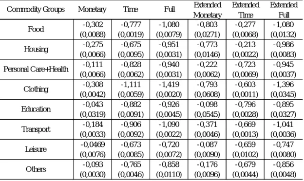
Therefore, another interpretation is that the tendency of being engaged in informal activities would also be due to the prices. Table 4 reports own-price elasticity results. Monetary and extended monetary based estimations show that households are more sensitive to price variation for necessary goods. Households’s reaction to changes in monetary prices of food, housing and clothing commodity groups apparently stronger than rest of the consumption groups. These results promise to expand the understanding of a person's motivation to participate in informal activities. The monetary price elasticities are more inelastic than the time ones. However, this tendency changes for extended estimation results. The simple fact is that households are more likely to compensate the loss due to prices changes, by increasing domestic activities and decreasing monetary expenses. Therefore, education, transport, personal care with health, leisure and other expenditures imply more inelastic price elasticity of demand. In this relation, compensation by time spent in domestic activities for these groups of commodities is low. This result is coherent with our income elasticity findings.
Table 4: Decomposition of Compensated Own-Price Elasticities (Standard Errors in
Parenthesis), Whole Population
-0,302 (0,0088) -0,777 (0,0019) -1,080 (0,0079) -0,803 (0,0271) -0,277 (0,0068) -1,080 (0,0132) -0,275 (0,0066) -0,675 (0,0095) -0,951 (0,0031) -0,773 (0,0146) -0,213 (0,0022) -0,986 (0,0083) -0,111 (0,0066) -0,828 (0,0062) -0,940 (0,0031) -0,222 (0,0062) -0,723 (0,0069) -0,945 (0,0037) -0,308 (0,0042) -1,111 (0,0059) -1,419 (0,0020) -0,793 (0,0608) -0,603 (0,0011) -1,396 (0,0345) -0,043 (0,0319) -0,882 (0,0091) -0,926 (0,0045) -0,098 (0,0545) -0,796 (0,0028) -0,895 (0,0327) -0,184 (0,0033) -0,906 (0,0092) -1,090 (0,0022) -0,371 (0,0046) -0,669 (0,0013) -1,041 (0,0036) -0,0469 (0,0076) -0,673 (0,0085) -0,720 (0,0072) -0,087 (0,0090) -0,659 (0,0102) -0,747 (0,0080) -0,093 (0,0030) -0,765 (0,0046) -0,858 (0,0110) -0,176 (0,0096) -0,679 (0,0044) -0,856 (0,0048) Commodity Groups Monetary
Others Full Extended Monetary Extended Time Extended Full Food Housing Time Personal Care+Health Clothing Education Transport Leisure
*Variance were corrected for generated repressors by bootstrap
Sources: Household Budget Survey (2003,2004, 2005,2006) Time Use Survey (2006)
Taken together, these results propose two main conclusions. The first conclusion deduced from income elasticity results explained above is that households may be more inclined to work because of shortage of certain consumption groups which have relatively low shares in the budget (i.e. because necessary goods expenditures take large part of household’s total expenditures). The second conclusion proposes that decreasing purchasing power due to an increase in prices for certain commodities forces households to compensate this loss by informal monetary spending and not by domestic activities.
4. Conclusion
Full price approach provide such estimates for different commodity groups in absence of real price data, solving in this way the problem of price data availability in most developing countries. In this work, aggregated commodity groups were analyzed from two different perspectives: at first, we measure monetary one and full expenditure one allows taking into account the domestic production of the household through the incorporation of time on family expenditures. Thus, the proposed enlarged version of Lyssiotou et al. allows the estimation of the size of the informal economy by estimation of the complete demand system using full prices obtained by matching of time use information and monetary expenditure data. Neglecting informal activities results in an underestimation of total output by 47.22% and 32.06% using full expenditure respectively for self-employed and wage earners (39.07% and 26.53% respectively for monetary expenditure only).
Further in this study, to measure demand elasticities we use full price method. Full price elasticities were decomposed in monetary price and time elasticities. Additional to this estimation, we re-measure demand elasticities for all populations and sub-populations, such as the self-employed and wage earners, by adding the under-reported earning part of household income into full prices. Elasticity results report that shortage of consumption of health with personal care, education, transport, leisure, other consumption groups stimulates participation in informal activities for two reasons. These groups of consumption relatively take lower shares; hence insufficient, in the budget than that of food, housing, clothing. A second reason is that households are less able to compensate their loss, due to price changes, by time spent in domestic activities. The model allows also the estimation on the importance of informal activities for different sub-populations to be used in public polices targeting poverty and inequality issues.
REFERENCES
Aktuna-Gunes, A.T., Starzec, C., Gardes, F. [2014], “Une évaluation de la taille de l’économie informelle par un système complet de demande estimé sur données monétaires et temporelles”, Revue Economique, 65 (4), p. 567-590.
Banks, J., Blundell, R., Lewbel, A. [1997], “Quadratic Engel Curves and Consumer Demand”, Review of Economic Studies, 89 (4), p. 527-539.
Becker, G. [1965], “A Theory of the Allocation of Time”, The Economic Journal, 75, p.493-517.
Canelas, C., Gardes, F., Salazar, S. [2013], A Microsimulation Based on Tax Reform,
Documents de Travail du Centre d’Economie de la Sorbonne (CES).
Cox, T.L., Wohlgenant M.K. [1986], “Prices and Quality Effects in Cross-Sectional Demand Analysis”, American Journal of Agricultural Economics, 68(4), p. 908–919
De Vany, A. [1974], “The Revealed Value of Time in Air Travel”, The Review of Economics
and Statistics, 56(1), p. 77–82.
Deaton, A., Muellbauer, J. [ 1980], “An Almost Ideal Demand System”, The American
Economic Review, 70(3), p. 312–326.
Fortin, B., Lacroix, G., Pinard, D. [2009], “Evaluation de l’économie souterraine au Québec: une approche micro-économétrique”, Revue Economique, 60 (5), p. 1257-1274.
Gardes, F. [2014], “Full Price Elasticities and the Opportunity Cost for Time”, CES
Documents de Travail du Centre d’Economie de la Sorbonne (CES)
Gardes, F., and C. Starzec. [2014], “Individual prices and household’s size: a restatement of equivalence scales using time and monetary expenditures combined”, Working Paper, Centre d’Economie de la Sorbonne (CES).
Gardes, F., Duncan, G.J., Gaubert, P., Starzec, C. [2005], “A Comparison of Consumption Models Estimated on American and Polish Panel and Pseudo-Panel data”, Journal of
Business and Economic Statistics, April, 23(2).
Lyssiotou, P., Pashardes, P., Stengos, T. [2004], “Estimates of the Black Economy based on Consumer Demand Approaches”¸ The Economic Journal, 114, p. 622-640.
Pashardes, P. [1993], “Bias in Estimating the Almost Ideal Demand System with the Stone Index Approximation”, The Economic Journal, 103(419), p. 908–915.
Pissarides, C., Webber, G. [1989], “An Expenditure-Based Estimate of Britain’s Black Economy”, Journal of Public Economics, 39, p. 17-32.
TURKISH STATISTICAL INSTITUTE [2006,2005,2004,2003], Household Budget Survey TURKISH STATISTICAL INSTITUTE [2006], Time Use Survey.
Appendix I
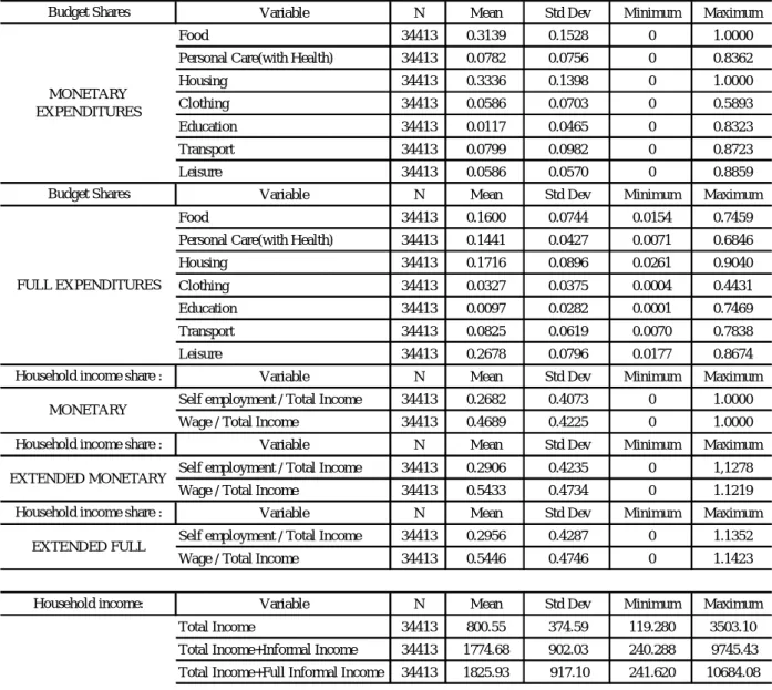
Table 5: Descriptive Statistics
Variable N Mean Std Dev Minimum Maximum
Food 34413 0.3139 0.1528 0 1.0000
Personal Care(with Health) 34413 0.0782 0.0756 0 0.8362
Housing 34413 0.3336 0.1398 0 1.0000
Clothing 34413 0.0586 0.0703 0 0.5893
Education 34413 0.0117 0.0465 0 0.8323
Transport 34413 0.0799 0.0982 0 0.8723
Leisure 34413 0.0586 0.0570 0 0.8859
Variable N Mean Std Dev Minimum Maximum
Food 34413 0.1600 0.0744 0.0154 0.7459
Personal Care(with Health) 34413 0.1441 0.0427 0.0071 0.6846
Housing 34413 0.1716 0.0896 0.0261 0.9040
Clothing 34413 0.0327 0.0375 0.0004 0.4431
Education 34413 0.0097 0.0282 0.0001 0.7469
Transport 34413 0.0825 0.0619 0.0070 0.7838
Leisure 34413 0.2678 0.0796 0.0177 0.8674
Variable N Mean Std Dev Minimum Maximum
Self employment / Total Income 34413 0.2682 0.4073 0 1.0000
Wage / Total Income 34413 0.4689 0.4225 0 1.0000
Variable N Mean Std Dev Minimum Maximum
Self employment / Total Income 34413 0.2906 0.4235 0 1,1278
Wage / Total Income 34413 0.5433 0.4734 0 1.1219
Variable N Mean Std Dev Minimum Maximum
Self employment / Total Income 34413 0.2956 0.4287 0 1.1352
Wage / Total Income 34413 0.5446 0.4746 0 1.1423
Variable N Mean Std Dev Minimum Maximum
Total Income 34413 800.55 374.59 119.280 3503.10
Total Income+Informal Income 34413 1774.68 902.03 240.288 9745.43
Total Income+Full Informal Income 34413 1825.93 917.10 241.620 10684.08
Budget Shares MONETARY EXPENDITURES FULL EXPENDITURES Budget Shares EXTENDED FULL Household income: Household income share : EXTENDED MONETARY
Household income share :
Household income share : MONETARY
Table 6: The estimation results of the Complete Demand System, self-employed, (GMM) 2003-2006
Variables Food t- ratio Pc+Health t- ratio Housing t- ratio Clothing t- ratio Education t- ratio Transport t- ratio Leisure t- ratio
Constant 24.27391 6.25 2.257977 1.19 18.80546 3.90 0.58871 0.49 0.216534 0.98 0.024431 0.02 2.737177 2.12
2003
2004 -0.40827 -6.76 0.037563 1.55 -0.11442 -2.08 0.044333 2.88 0.010848 3.48 0.055612 2.74 0.03008 1.82
2005 -0.03954 -1.37 0.031155 3.82 0.119515 5.58 0.009577 1.88 -0.00163 -1.60 0.023678 3.48 0.030596 5.50
2006 -0.25349 -5.84 0.002037 0.26 -0.02741 -0.80 0.019118 1.94 0.003224 1.68 0.014075 1.09 0.006037 0.57
Number of households members 0.022113 4.83 -0.00726 -3.24 -0.02492 -4.93 -0.00282 -1.98 -0.00078 -2.79 -0.0067 -3.53 -0.00555 -3.62
Home ownership 0.052861 4.71 -0.01803 -3.72 -0.00186 -0.19 -0.00441 -1.40 -0.00136 -1.72 -0.01167 -2.79 -0.0106 -3.20
Husband in white collar occupation 0.172647 5.37 -0.00415 -0.27 0.083627 2.36 0.001115 0.11 -0.00412 -1.99 -0.01296 -1.01 0.002538 0.24
Husband in blue collar occupation 0.192601 6.27 0.017928 1.19 0.152495 3.83 0.005384 0.56 -0.00111 -0.61 -0.00454 -0.36 0.016018 1.56
Wife in blue collar occupation -0.12797 -3.69 -0.01699 -0.98 -0.07682 -2.08 -0.00529 -0.48 -0.00007 -0.03 -0.00233 -0.16 -0.00641 -0.54
Wife in white collar occupation -0.25524 -4.89 -0.00525 -0.23 -0.13052 -2.64 0.015658 1.06 0.00831 2.39 0.024395 1.24 0.008256 0.52
Wife worker at the company (under 10 worker) 0.339502 6.71 -0.0576 -2.95 0.007589 0.19 -0.04767 -3.83 -0.00979 -3.81 -0.06622 -4.07 -0.03946 -2.97
Area (urban = 1) -0.30155 -7.45 0.113411 7.78 0.222445 6.33 0.044899 4.85 0.014464 7.04 0.064267 5.28 0.07434 7.50
Husband wage worker -0.1534 -2.17 0.234035 7.78 0.386199 4.59 0.127337 6.79 0.027751 6.43 0.179113 7.29 0.156177 7.60
Wife wage worker -0.03142 -0.99 0.061801 4.17 0.048456 1.61 0.026465 2.76 0.00402 1.85 0.045285 3.55 0.020819 2.04
Husband with out contract -0.01624 -0.21 0.221245 6.59 0.486511 4.86 0.13611 6.54 0.029004 6.24 0.171558 6.26 0.164472 7.19
Computer -0.10364 -4.33 -0.02144 -1.84 -0.12747 -4.46 -0.01218 -1.64 0.005288 3.06 -0.00393 -0.40 -0.0022 -0.28
Car 0.005434 0.39 0.000756 0.11 -0.00844 -0.56 0.002432 0.58 -0.00018 -0.19 0.069203 12.19 0.004728 1.04
Good heating system -0.09763 -5.70 0.005823 0.87 0.028374 2.00 0.009918 2.28 0.00437 3.91 0.008768 1.52 0.006399 1.38
Number of rooms in the house 0.015125 1.68 -0.00432 -1.04 0.015079 1.75 0.000061 0.02 -0.00026 -0.49 -0.00399 -1.13 -0.00005 -0.02
Children under than 16 years old -0.07046 -3.60 0.037755 4.89 0.071188 3.90 0.028283 5.75 0.005597 5.10 0.03148 4.82 0.027281 5.17
yr -17.2272 -5.31 -5.39331 -3.13 -19.8602 -3.85 -2.44508 -2.26 -0.1722 -0.86 -3.00981 -2.11 -3.45851 -2.94 yr2 31.06959 3.19 25.3528 4.97 69.98399 4.26 13.60385 4.28 1.786873 2.99 17.40005 4.13 16.81772 4.85 yr3 -13.5456 -1.96 -20.1576 -5.84 -50.4423 -4.41 -11.2943 -5.26 -1.63369 -3.96 -14.5758 -5.10 -13.4833 -5.75 Y -5.65383 -6.05 -0.47894 -1.05 -4.44109 -3.84 -0.13272 -0.46 -0.04065 -0.76 0.01878 0.05 -0.62874 -2.02 Y2 0.335709 6.01 0.026509 0.97 0.261863 3.83 0.007292 0.43 0.002471 0.77 -0.00239 -0.11 0.037114 2.00 Full Price 0.019172 1.22 -0.04846 -37.69 -0.09752 -7.33 -0.03289 -75.20 -0.02225 -14.94 -0.03163 -46.65 -0.03425 -40.53
Under-reporting Self-employment (Yr) t ratio
k (under reporting ratio for yr ) 5.00
Stock-Yogo weak ID test (endogenous regressor: income) >5% >10% >20%
Minimum eigenvalue statistic -F( 17, 26173) = 15,36 21,31 11,49 6,36 Parameter 1.58 (Critical values)2SLS relative bias - -- - - -
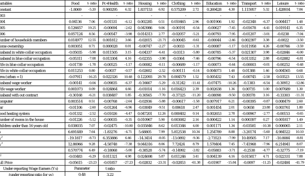
-Table 7: The estimation results of the Complete Demand System, wage earners, (GMM) 2003-2006
Variables Food t- ratio Pc+Health t- ratio Housing t- ratio Clothing t- ratio Education t- ratio Transport t- ratio Leisure t- ratio
Constant -1.8069 -5.20 0.900295 6.32 1.837153 6.92 0.575209 2.72 0.269428 4.30 1.115957 5.32 1.428934 7.84
2003
2004 0.04136 7.06 -0.01531 -6.12 0.002285 0.51 0.010465 2.96 0.001906 1.92 -0.02348 -6.37 0.004417 1.48
2005 0.126657 19.25 -0.00694 -2.62 0.043986 9.06 -0.00191 -0.54 -0.00627 -7.45 -0.01678 -4.41 0.019141 6.35
2006 0.057124 8.56 -0.00547 -3.98 0.014313 2.77 -0.02057 -5.21 -0.00793 -7.95 -0.01207 -3.01 -0.0238 -7.04
Number of households members 0.014977 12.55 0.001812 3.66 -0.02015 -21.71 -0.00045 -0.61 -0.00044 -2.46 0.002397 3.38 -0.0022 -3.50
Home ownership 0.003051 0.71 0.000028 0.01 -0.00747 -2.27 -0.0033 -1.31 -0.00087 -1.17 0.011958 4.26 -0.00766 -3.59
Husband in white collar occupation -0.05035 -5.98 0.011505 3.15 -0.04337 -6.41 -0.0313 -5.80 -0.00785 -5.37 0.021307 3.98 -0.02846 -6.00
Husband in blue collar occupation -0.05311 -7.08 0.013304 4.16 -0.02355 -3.98 -0.0364 -7.46 -0.00796 -6.54 0.013352 2.88 -0.02882 -6.81
Wife in blue collar occupation -0.01739 -1.78 -0.00525 -1.17 -0.00082 -0.11 -0.00689 -1.17 -0.00073 -0.44 -0.00003 -0.01 -0.00252 -0.48
Wife in white collar occupation 0.011253 0.80 -0.0037 -0.57 -0.02602 -2.52 -0.00111 -0.14 0.004073 1.48 0.01388 1.46 0.004565 0.68
Area (urban = 1) -0.07911 -16.25 0.022326 10.48 0.122093 29.78 0.004579 1.52 0.005432 7.43 -0.00745 -2.58 0.03523 13.55
Husband wage worker -0.00141 -0.04 -0.09835 -6.37 -0.16667 -5.29 -0.31242 -11.41 -0.07475 -10.26 -0.1383 -6.54 -0.30912 -12.86
Wife wage worker 0.001073 0.09 0.024864 4.66 -0.01014 -1.16 0.016423 2.39 0.002638 1.36 0.00735 1.00 0.007689 1.30
Husband with out contract -0.30168 -6.21 0.038487 1.85 -0.30565 -7.70 -0.37325 -11.20 -0.08098 -9.50 0.09378 3.16 -0.33303 -11.31
Computer 0.003514 0.51 -0.00768 -2.64 -0.02936 -5.88 -0.00617 -1.58 0.007917 6.21 -0.00395 -0.87 0.008479 2.60
Car -0.01106 -2.60 -0.01264 -6.96 -0.03049 -9.51 0.00618 2.47 0.001454 2.01 0.0658 23.88 0.003761 1.80
Good heating system -0.01332 -2.52 -0.01026 -4.47 0.047201 12.26 0.000402 0.14 0.002653 2.78 -0.00967 -2.77 -0.00153 -0.65
Number of rooms in the house -0.01226 -5.12 -0.00035 -0.35 0.010967 5.90 0.003082 2.16 0.000422 1.14 0.000397 0.27 0.001817 1.49
Children under than 16 years old 0.038035 7.07 -0.02475 -10.80 0.035846 8.62 0.013346 4.00 0.001171 1.34 -0.03581 -10.38 0.006065 2.11
ys 6.691449 7.64 -1.83276 -4.71 5.68805 7.99 5.812538 10.34 1.254789 8.88 -3.20174 -5.60 4.984522 10.10 ys2 -19.1817 -8.73 6.353886 6.46 -14.3414 -8.05 -13.0892 -9.36 -2.73523 -7.99 10.49505 7.17 -10.8084 -8.81 ys3 12.86966 9.28 -4.58748 -7.38 9.044316 8.06 7.72424 8.79 1.578404 7.45 -7.41968 -7.96 6.214941 8.07 Y 0.570774 6.49 -0.18068 -5.00 -0.38528 -5.74 -0.14992 -2.82 -0.05883 -3.71 -0.2538 -4.77 -0.32775 -7.19 Y2 -0.03483 -6.29 0.011321 4.98 0.024698 5.87 0.011246 3.41 0.004139 4.16 0.015817 4.71 0.022331 7.88 Full Price -0.05615 -23.23 -0.01857 -27.23 -0.02832 -23.31 -0.02853 -61.38 -0.01907 -15.84 -0.0097 -11.25 -0.02484 -41.79
Under-reporting Wage Earners (Ys) t ratio
t under reporting ratio for ys ) 3.22
-
-Parameter 0.48
-Table 8: The estimation results of the Complete Demand System, full expenditure, self-employed, (GMM) 2003-2006
Variables Food t- ratio Pc+Health t- ratio Housing t- ratio Clothing t- ratio Education t- ratio Transport t- ratio Leisure t- ratio
Constant -0.47579 -6.16 -0.22907 -6.91 -0.01809 -0.63 0.001717 0.13 -0.19759 -4.98 0.002532 0.07 0.117357 1.34
2003
2004 0.005366 5.12 0.00131 3.17 0.001561 9.75 -0.00006 -0.67 -0.00037 -0.87 -0.00004 -0.17 0.004219 6.68
2005 0.075348 130.78 0.235708 1567.72 0.056245 378.89 0.010434 232.19 0.005639 46.48 0.091672 576.20 0.524302 1752.13
2006 0.091984 118.71 0.112093 872.83 0.066723 365.40 0.021827 255.93 0.021384 57.70 0.089508 413.82 0.485875 784.76
Number of households members 0.000214 3.60 -0.00002 -0.72 0.000133 5.15 0.000272 17.25 0.000162 3.89 -0.00009 -2.48 -0.00085 -10.05
Home ownership -0.00051 -2.85 0.000191 2.26 0.000186 3.15 -0.00004 -1.49 -0.00046 -4.44 -0.00022 -2.63 0.000178 0.89
Husband in white collar occupation 0.000059 0.13 -0.00014 -0.65 0.000102 0.79 0.000401 6.09 0.000914 3.54 0.000941 4.45 -0.00242 -5.01
Husband in blue collar occupation -0.00216 -5.35 -0.00121 -6.63 -0.00006 -0.31 0.000209 2.83 -0.00041 -1.73 0.000686 3.00 -0.00064 -1.28
Wife in blue collar occupation -0.00161 -3.17 0.000481 2.37 0.000063 0.41 -0.00003 -0.36 -0.00032 -1.72 -0.00018 -0.69 -0.00144 -2.65
Wife in white collar occupation 0.003334 4.60 0.001897 5.53 0.000139 0.56 0.00005 0.41 0.001415 3.93 0.000547 1.38 -0.00183 -2.15
Area (urban = 1) 0.001821 1.98 0.00047 0.99 -0.00195 -6.23 -0.0007 -8.63 -0.00124 -2.99 -0.00024 -0.94 0.005279 8.22
Husband wage worker -0.00175 -1.50 -0.0028 -3.53 -0.00168 -2.61 -0.00111 -4.69 -0.00424 -5.45 0.000948 1.39 0.010077 6.26
Wife wage worker 0.002726 4.45 0.000821 3.81 -0.00014 -0.85 -0.0001 -1.24 0.000284 1.27 0.000688 2.61 0.000818 1.39
Husband with out contract -0.00499 -3.25 -0.0048 -4.35 -0.00207 -2.44 -0.00084 -2.67 -0.00446 -4.08 0.00142 1.59 0.010083 4.78
Computer 0.002619 5.70 0.001109 4.56 0.000618 3.22 0.000231 2.73 0.001296 4.96 -0.00025 -0.95 -0.00167 -2.88
Car 0.00009 0.53 -0.00022 -2.87 -0.00005 -0.73 0.000072 2.23 -0.00003 -0.39 0.000565 5.16 -0.00009 -0.40
Good heating system 0.001718 5.81 0.000315 3.35 0.00066 8.35 0.000109 2.65 0.000485 4.16 0.00012 1.02 -0.00031 -1.12
Number of rooms in the house -0.00022 -1.74 -0.00015 -3.06 0.000109 2.79 0.000041 1.89 -0.00006 -0.93 -0.00007 -1.07 -0.00006 -0.37
Children under than 16 years old 0.00074 2.29 -0.00049 -3.09 8.832E-6 0.07 -0.00004 -0.84 0.000337 2.43 0.000625 4.54 0.000444 1.51 ys 0.104193 2.42 0.104346 4.70 0.036787 1.51 -0.02494 -3.24 -0.03198 -1.20 -0.15964 -6.60 0.099148 1.88 ys2 -0.08883 -0.68 -0.33169 -4.61 -0.15795 -1.81 0.030453 1.26 0.015413 0.21 0.531028 6.94 0.081203 0.50 ys3 -0.02707 -0.28 0.225393 4.33 0.122086 1.91 -0.0059 -0.35 0.011146 0.22 -0.37783 -7.05 -0.17771 -1.56
Y 0.119832 6.12 0.057348 6.73 0.004231 0.58 -0.00016 -0.05 0.051246 5.08 0.000975 0.10 -0.03366 -1.52
Y2 -0.00735 -6.06 -0.00353 -6.66 -0.00022 -0.50 0.000012 0.06 -0.0032 -5.12 -0.00015 -0.25 0.002118 1.55
Full Price -0.00302 -7.71 0.000287 3.79 0.000346 3.34 -0.0001 -12.15 7.788E-6 0.12 0.000056 1.41 0.000305 4.38
Under-reporting Self-employment (Yr) t ratio kunder reporting ratio for yr ) 2.24
-
-Parameter 1.91
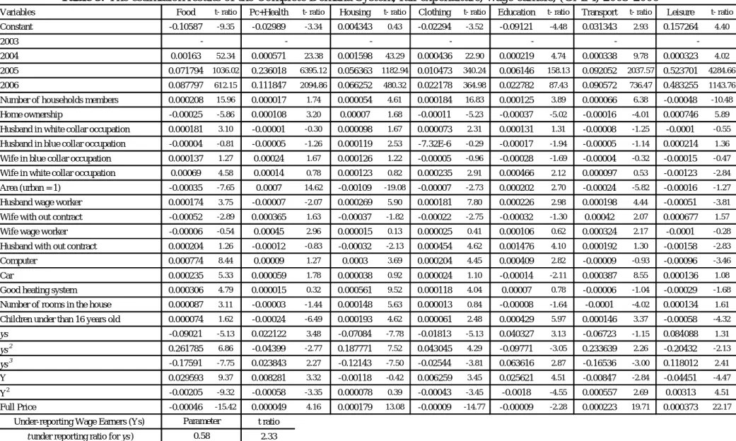
-Table 9: The estimation results of the Complete Demand System, full expenditure, wage earners, (GMM) 2003-2006
Variables Food t- ratio Pc+Health t- ratio Housing t- ratio Clothing t- ratio Education t- ratio Transport t- ratio Leisure t- ratio
Constant -0.10587 -9.35 -0.02989 -3.34 0.004343 0.43 -0.02294 -3.52 -0.09121 -4.48 0.031343 2.93 0.157264 4.40
2003
2004 0.00163 52.34 0.000571 23.38 0.001598 43.29 0.000436 22.90 0.000219 4.74 0.000338 9.78 0.000323 4.02
2005 0.071794 1036.02 0.236018 6395.12 0.056363 1182.94 0.010473 340.24 0.006146 158.13 0.092052 2037.57 0.523701 4284.66
2006 0.087797 612.15 0.111847 2094.86 0.066252 480.32 0.022178 364.98 0.022782 87.43 0.090572 736.47 0.483255 1143.76
Number of households members 0.000208 15.96 0.000017 1.74 0.000054 4.61 0.000184 16.83 0.000125 3.89 0.000066 6.38 -0.00048 -10.48
Home ownership -0.00025 -5.86 0.000108 3.20 0.00007 1.68 -0.00011 -5.23 -0.00037 -5.02 -0.00016 -4.01 0.000746 5.89
Husband in white collar occupation 0.000181 3.10 -0.00001 -0.30 0.000098 1.67 0.000073 2.31 0.000131 1.31 -0.00008 -1.25 -0.0001 -0.55
Husband in blue collar occupation -0.00004 -0.81 -0.00005 -1.26 0.000119 2.53 -7.32E-6 -0.29 -0.00017 -1.94 -0.00005 -1.14 0.000214 1.36
Wife in blue collar occupation 0.000137 1.27 0.00024 1.67 0.000126 1.22 -0.00005 -0.96 -0.00028 -1.69 -0.00004 -0.32 -0.00015 -0.47
Wife in white collar occupation 0.00069 4.58 0.00014 0.78 0.000123 0.82 0.000235 2.91 0.000466 2.12 0.000097 0.53 -0.00123 -2.84
Area (urban = 1) -0.00035 -7.65 0.0007 14.62 -0.00109 -19.08 -0.00007 -2.73 0.000202 2.70 -0.00024 -5.82 -0.00016 -1.27
Husband wage worker 0.000174 3.75 -0.00007 -2.07 0.000269 5.90 0.000181 7.80 0.000226 2.98 0.000198 4.44 -0.00051 -3.81
Wife with out contract -0.00052 -2.89 0.000365 1.63 -0.00037 -1.82 -0.00022 -2.75 -0.00032 -1.30 0.00042 2.07 0.000677 1.57
Wife wage worker -0.00006 -0.54 0.00045 2.96 0.000015 0.13 0.000025 0.41 0.000106 0.62 0.000324 2.17 -0.0001 -0.28
Husband with out contract 0.000204 1.26 -0.00012 -0.83 -0.00032 -2.13 0.000454 4.62 0.001476 4.10 0.000192 1.30 -0.00158 -2.83
Computer 0.000774 8.44 0.00009 1.27 0.0003 3.69 0.000204 4.45 0.000409 2.82 -0.00009 -0.93 -0.00096 -3.46
Car 0.000235 5.33 0.000059 1.78 0.000038 0.92 0.000024 1.10 -0.00014 -2.11 0.000387 8.55 0.000136 1.08
Good heating system 0.000306 4.79 0.000015 0.32 0.000561 9.52 0.000118 4.04 0.00007 0.78 -0.00006 -1.04 -0.00029 -1.68
Number of rooms in the house 0.000087 3.11 -0.00003 -1.44 0.000148 5.63 0.000013 0.84 -0.00008 -1.64 -0.0001 -4.02 0.000134 1.61
Children under than 16 years old 0.000074 1.62 -0.00024 -6.49 0.000193 4.62 0.000061 2.48 0.000429 5.97 0.000146 3.37 -0.00058 -4.32
ys -0.09021 -5.13 0.022122 3.48 -0.07084 -7.78 -0.01813 -5.13 0.040327 3.13 -0.06723 -1.15 0.084088 1.31 ys2 0.261785 6.86 -0.04399 -2.77 0.187771 7.52 0.043045 4.29 -0.09771 -3.05 0.233639 2.26 -0.20432 -2.13 ys3 -0.17591 -7.75 0.023843 2.27 -0.12143 -7.50 -0.02544 -3.81 0.063616 2.87 -0.16536 -3.00 0.118012 2.41 Y 0.029593 9.37 0.008281 3.32 -0.00118 -0.42 0.006259 3.45 0.025621 4.51 -0.00847 -2.84 -0.04451 -4.47 Y2 -0.00205 -9.32 -0.00058 -3.35 0.000078 0.39 -0.00043 -3.45 -0.0018 -4.55 0.000557 2.69 0.00313 4.51 Full Price -0.00046 -15.42 0.000049 4.16 0.000179 13.08 -0.00009 -14.77 -0.00009 -2.28 0.000223 19.71 0.000373 22.17
Under-reporting Wage Earners (Ys) t ratio
t under reporting ratio for ys ) 2.33
-
-Parameter 0.58
-Table 10: -Tables description and the details of selected instruments
The estimation of the model for full expenditure and exclusive monetary expenditure from the pooled cross-sectional data covering the period of investigation 2003-2006, for self-employed and wage earners are presented respectively in Tables 3.5-3.8. The size of the pooled sample increases to 34 414 households.
The proposed instruments were: the age of husband and wife, marital status, number of children, children more than 16 years old, owing house-related debt, household head being bound by an open-ended working contract, daily working occupation for household head, education status of the household head, having access to an internet connection, owning a television, refrigerator, oven.
The control variables included in the model are: the number of households members, the number of rooms in the house, home ownership, the number of children under 16 years old, physical environment (urban or rural), husband in blue collar occupation, husband in white collar occupation, wife in blue collar occupation, wife in white collar occupation, wife worker at the company (under 10 workers), husband wage worker, husband without working contract, wife wage worker and the durable goods dummies such as owning a computer, car ownership, having a good heating system.
Appendix II
Computation of the Under-Reported Ratio Both for the Self-Employed and Wage Earners
Once equation (4) has been applied, the estimated parameters of the Engel curves are used for the calculation of self-employed and wage earners’ true incomes as
* , m m m m s r Y Y
where Yr*and Ys* are the adjusted self-employed and wage earners' incomes obtained by multiplying their monetary (i.e. declared) incomes Y and r Y with corresponding under-sreported parameters and r . For the self-employed s is equal to r
ˆ , ˆ 10 1 R m m m a s r r y n y
and for wage earners is sˆ , ˆ 10 1 R m m m a r s s y n y
These under-reported parameters are calculated for each consumer group by using the estimated parameters of the complete demand system given in the equation (4) 1.
1 ˆ
Ris defined in terms of the quadratic model as
3 2 2 , 1 ˆ ˆ ˆ ˆ ˆ ˆ ˆ ˆ ˆ i 2 i (( i 2 i) 4 i( iln h i(ln h) (ˆi ˆij jh in( r s)n ˆt t) j n t R Y Y Z y A