HAL Id: halshs-00754295
https://hal-pjse.archives-ouvertes.fr/halshs-00754295
Submitted on 31 May 2020
HAL is a multi-disciplinary open access archive for the deposit and dissemination of sci-entific research documents, whether they are pub-lished or not. The documents may come from
L’archive ouverte pluridisciplinaire HAL, est destinée au dépôt et à la diffusion de documents scientifiques de niveau recherche, publiés ou non, émanant des établissements d’enseignement et de
Solving heterogeneous-agent models with paramaterized
cross-sectional distribution
Yann Algan, Olivier Allais, Wouter J. den Haan
To cite this version:
Yann Algan, Olivier Allais, Wouter J. den Haan. Solving heterogeneous-agent models with parama-terized cross-sectional distribution. Journal of Economic Dynamics and Control, Elsevier, 2008, 32 (3), pp.875-908. �10.1016/j.jedc.2007.03.007�. �halshs-00754295�
SOLVING HETEROGENEOUS-AGENT
MODELS WITH PARAMETERIZED
CROSS-SECTIONAL DISTRIBUTIONS
Yann ALGAN, Oliver ALLAIS, and Wouter J. DEN HAAN
March 16, 2007
Abstract
A new algorithm is developed to solve models with heterogeneous agents and aggregate uncertainty. Projection methods are the main building blocks of the algorithm and— in contrast to the most popular solution procedure— simulations only play a very minor role. The paper also develops a new simulation procedure that not only avoids cross-sectional sampling variation but is 10 (66) times faster than simulating an economy with 10,000 (100,000) agents. Because it avoids cross-sectional sampling variation, it can generate an accurate representation of the whole cross-sectional distribution. Finally, the paper outlines a set of accuracy tests.
Key Words: Incomplete markets, numerical solutions, projection methods, simulations
JEL Classi…cation: C63, D52
Algan: Paris School of Economics, University of Marne La Vallée; [email protected]. Allais: INRA, Corela; [email protected]. Den Haan: University of Amsterdam, London Business School, and CEPR; [email protected]. The authors would like to thank Chris Carroll, Ken Judd, Michel Juillard, Michael Reiter, and two anonymous referees for useful comments.
1
Introduction
Models with heterogeneous agents and aggregate uncertainty are becoming increas-ingly important. They not only improve the predictions of representative agent models, they also make it possible to study the behavior of sub groups in a general equilibrium framework. Solving such models is di¢ cult, because the set of state variables contains the cross-sectional distribution of agents’characteristics, which is a time-varying in…nite dimensional object in the presence of aggregate uncertainty. The most commonly used algorithm summarizes the cross-sectional distribution with a …nite set of moments and calculates the transition law for these state variables using a simulation procedure.1 This algorithm is relatively easy to implement and has been used to solve a variety of models. Nevertheless, it is important to have alternative algorithms. First, if an alternative algorithm generates a very similar numerical solution then this builds con…dence in the generated results. Accuracy checks are of course also helpful in this respect but accuracy tests have its limits. It is especially di¢ cult to test in all possible dimensions if the model has many dimensions. For complex models it is not uncommon that the results of some tests are not that great. If they occur in dimensions that are deemed not that important for the main properties of the model, we typically argue that it is not worth the extra computing time to …x the problem and sometimes it may not even be feasible. The problem is that it is very hard to determine whether inaccuracies in some parts of the model do not spill over to other more important parts or whether tiny but systematic inaccuracies do not accumulate to something more important. It is therefore important if one can replicate results using algorithms that uses di¤erent methodologies. The second reason to develop multiple algorithms is that di¤erent algorithms have di¤erent strenghts and weaknesses and so one type of algorithm may be more suitable for a particular problem.
The algorithm developed in this paper to solve models with heterogenous agents and aggregate uncertainty is quite di¤erent from the popular simulations-based al-gorithm in that simulations only play a minor role. In particular, simulation pro-cedures are not used to obtain the aggregate law of motion. Like Den Haan (1997) and Reiter (2002), we parameterize the cross-sectional distribution, which makes it possible to obtain a numerical solution using standard quadrature and projection techniques. Our algorithm has important e¢ ciency gains over the algorithms devel-oped in these two papers. In particular, we follow Reiter (2002) in using reference moments to get a better characterization of the cross-sectional distribution without increasing the number of state variables, but we do so in a way that is much more
tractable.
Two elements of the algorithm are likely to be useful in other applications as well. First, to obtain reference moments we need to simulate the economy and we develop a simulation procedure that avoids cross-sectional sampling uncertainty. Second, we propose a particular class of parameterizing densities that makes the problem of …nding the coe¢ cients that correspond to a set of moments a convex optimization problem. Using this class of functions avoids the need for good starting values, whereas for other functional forms we found this to be a major concern. Linking moments with a parameterized density is part of our simulation procedure and also plays a key role in the solution algorithm itself.
The standard simulation procedures constructs a panel of NT observations and
NN agents. By parameterizing the cross-sectional distribution and using quadrature
integration, however, our procedure can generate an accurate simulation with a con-tinuum of agents. Note that models with a large number of heterogeneous agents almost always assume a continuum of agents, so that the law of large numbers en-sures that idiosyncratic risk is averaged out. In fact, the assumption of a continuum of agents plays a key role, not only in the speci…cation of the state variables and the de…nition of the equilibrium, but also in the construction of most algorithms.2
Thus, by simulating with a continuum instead of a …nite number of agents, we stay much closer to the actual model being solved.
Our simulation procedure not only avoids cross-sectional sampling variation, it is also much cheaper. We found that simulating an economy with 10,000 agents for 1000 periods took 13 times as long as simulating the same economy with a continuum of agents. In our own algorithm, the simulation procedure only plays a very minor role. This is, of course, no reason not to use a more accurate simulation procedure. For algorithms that use a simulation procedure to calculate the aggregate law of motion, however, the improved simulation procedure will have bigger bene…ts.
The rest of this paper is organized as follows. The next section describes the production economy of Krusell and Smith (1998). Section 3 brie‡y discusses existing algorithms and summarizes the contributions of this paper. Section 4 describes the algorithm in detail and Section 5 describes the simulation procedure. Section 6 discusses how to check for accuracy and reports the results. The last section concludes.
2In particular, a crucial property being used is that conditional on realizations of the aggregate
shock and this period’s cross-sectional distribution, next period’s cross-sectional distribution is known with certainty.
2
The production economy
The economy is a production economy with aggregate shocks in which agents face di¤erent employment histories and partially insure themselves through (dis)saving in capital. For more details see Krusell and Smith (1998).
Problem for the individual agent. The economy consists of a unit mass of ex ante identical households. Each period, agents face an idiosyncratic shock " that determines whether they are employed, " = 1, or unemployed, " = 0. An employed agent earns a wage rate of $t: An employed agent earns an after-tax wage rate of
(1 t)$t and an unemployed agent receives unemployment bene…ts $t. Markets
are incomplete and the only investment available is capital accumulation. The net rate of return on this investment is equal to rt , where rt is the rental rate and
is the depreciation rate. Agent’s i maximization problem is as follows: max fci t;kit+1g1t=0 EP1t=0 t(c i t) 1 1 1 s.t. cit+ kt+1i = rtkti+ (1 t)$tl"it+ $t(1 "it) + (1 )kit ki t+1 0 (1) Here ci
t is the individual level of consumption, kit is the agent’s beginning-of-period
capital, and l is the time endowment.
Firm problem. Markets are competitive and the production technology of the …rm is characterized by a Cobb-Douglas production function. Consequently, …rm heterogeneity is not an issue. Let Kt and Lt stand for per capita capital and the
employment rate, respectively. Per capita output is given by
Yt= atKt(lLt)1 (2) and prices by $t= (1 ) at( Kt lLt ) (3) rt= at( Kt lLt ) 1 (4)
Aggregate productivity, at, is an exogenous stochastic process that can take on two
Government The only role of the government is to tax employed agents and to redistribute funds to the unemployed. We assume that the government’s budget is balanced each period. This implies that the tax rate is equal to
t =
ut
lLt
: (5)
where ut= 1 Lt denotes the unemployment rate in period t.
Exogenous driving processes. There are two stochastic driving processes. The …rst is aggregate productivity and the second is the employment status. Both are assumed to be …rst-order Markov processes. We let aa0""0 stand for the probability
that at+1 = a0 and "it+1= "0 when at= a0 and "it= "0. These transition probabilities
are chosen such that the unemployment rate can take on only two values. That is, ut = ub when at= ab and ut= ug when at= ag with ub > ug.
Equilibrium. Krusell and Smith (1998) consider recursive equilibria in which the policy functions of the agent depend on his employment status, "i, his
beginning-of-period capital holdings, ki, aggregate productivity, a, and the cross-sectional
distribution of capital holdings. An equilibrium consists of the following. Individual policy functions that solve the agent’s maximization problem. A wage and a rental rate that are determined by 3 and 4, respectively.
A transition law for the cross-sectional distribution of capital, that is consistent with the investment policy function.
3
Relation to existing algorithms
In this paper we give a brief overview of existing algorithms and then highlight the contributions of this paper.
3.1
Existing algorithms
A standard aspect of numerical algorithms that solve models with heterogeneous agents is to summarize the in…nite-dimensional cross-sectional distribution of agents’ characteristics by a …nite set of moments, m. The transition law is then a mapping that generates next period’s moments, m0, given the values of the moments in the current period, m, and the realization of the aggregate shock. Den Haan (1996),
Krusell and Smith (1998), and Rios-Rull (1997) propose to calculate this transition law as follows. First, construct a time series for the cross-sectional moments by simulating an economy with a large but …nite number of agents. Second, regress the simulated moments on the set of state variables. The …rst disadvantage of the simulation procedure is that moments are calculated using Monte Carlo integration, which is known to be an ine¢ cient numerical integration procedure.3 The second
disadvantage is that the observations are clustered around the mean, since they are taken from a simulated series. An e¢ cient projection procedure, however, requires the explanatory variables to be spread out, for example, by using Chebyshev nodes.4
Consequently, the use of simulation procedures may make it expensive (in terms of computing time) to obtain an accurate solution, especially if one wants the solution to be accurate across the whole state space.
Den Haan (1997) parameterizes the cross-sectional distribution with a ‡exible functional form, P (k; ), which makes it possible to use quadrature techniques to do the numerical integration. In addition, his algorithm uses Chebyshev nodes to construct a grid of explanatory variables for the projection step. The coe¢ cients of the approximating density, , are pinned down by the set of moments used, m. The disadvantage of Den Haan (1997) is that the shape of the distribution is completely pinned down by the moments used as state variables and the class of ‡exible functional forms used. Consequently, a large number of state variables may be needed to get the shape of the cross-sectional distribution right even when just a few moments actually matter for agents’ behavior. Another drawback of Den Haan (1997) is that an ine¢ cient procedure is used to …nd the coe¢ cients of the approximating density. Reiter (2002) improves upon the algorithm of Den Haan (1997) in an ingenious way by letting the shape of the distribution depend not only on the moments used as state variables, m; but also on a set of reference moments that are obtained by a simulation procedure.
Promising recent alternatives to the standard algorithm have been developed in Preston and Roca (2006) and Reiter (2006). Reiter (2006) …rst solves a model with-out aggregate uncertainty using standard projection procedures. Next, by replacing the endogenous variables in the equations of the model with the parameterized nu-merical solution, he obtains a di¤erence equation in the nunu-merical coe¢ cients. Then he uses perturbation techniques to solve for the sensitivity of the numerical solution to aggregate shocks. This is quite a di¤erent approach then the procedure used here, which is good for the profession, because the more variety among available approaches used the better. Preston and Roca (2006) use a "pure" perturbation
3See Judd (1998).
method to solve the model.5 Perturbation methods are likely to work well when
the distribution needs to be characterized by many statistics, because dealing with many arguments is the strength of perturbation methods.
3.2
The contributions of this paper
The main contributions of this paper are the following.
Calculating the transition law of the cross-sectional distribution. The
disadvantage of Reiter (2002) is that the particular implementation of the idea of reference moments is very cumbersome.6 As in Den Haan (1997) and Reiter (2002),
this paper develops a procedure to calculate this transition law without relying on simulation procedures to calculate moments and to carry out the projection step. As in Reiter (2002), it uses reference moments, but the modi…cations introduced make the procedure much more straightforward to implement. In other words, the algorithm is an important improvement over earlier attempts that use projection methods to solve models with heterogeneous agents. Moreover, because the building blocks are so di¤erent from the simulation procedures, it provides a constructive alternative.
Calculating the approximating density for given moments. The algorithm
links a set of moments with a parameterized density. Consequently, an important part of the algorithm is the mapping between the set of moments and the coe¢ cients of the density. One possibility would be to use an equation solver that chooses the set of coe¢ cients so that the moments of the parameterized density are equal to the speci…ed moments. We found this procedure to be slow and intermittently breaking down. By choosing a particular choice for the basis functions of the approximating
5They replace the inequality constraint with a penalty function, since perturbation methods
cannot deal well with the kind of inequality constraint used here. This also accomplishes that agents do not have negative capital holdings and try to stay away from low capital stocks.
6Reiter (2002) constructs a reference density G(m), which relates the shape of the distribution
to the set of moments that serve as state variables. It is a weighted average of distributions from a simulated economy, where distributions with moments closer to m get more weight. Step functions are used to construct a reference distribution, which has the advantage of being very ‡exible but has the disadvantage of using a lot of parameters. One problem of the approach in Reiter (2002) is that the moments of the reference density may not be equal to m. This means that one …rst has to apply operations to ensure that one obtains a new reference function eG(m) for which this is not the case. But even if m contains only …rst and second moments, then this problem entails more than a linear transformation, since eG(m) has to be a step function that conforms to the speci…ed grid and cannot violate the constraints on the support of the distribution, such as the constraint
polynomial we transform this problem into a convex optimization problem, for which reliable convergence algorithms exist. This procedure is likely to be useful outside the literature of numerical solution techniques, since characterizing a cross-sectional distribution with a CDF from a class of ‡exible functional forms is a common prob-lem in econometrics.
Simulating a panel without cross-sectional sampling variation. This
pa-per develops a procedure to simulate an economy without cross-sectional sampling variation. Standard procedure is to simulate data using a …nite number of agents and a …nite number of time periods, which means that the outcome depends on the particular random draw used. Sampling variation disappears at a slow rate and could be especially problematic if the number of a particular type of agent is small relative to the total number of agents.
Existing models with a large number of heterogeneous agents typically assume that there is a continuum of agents. This implies that conditional on the realization of the aggregate shock there is no cross-sectional sampling variation, a property that plays a key role in the de…nition of the set of state variables and the de…nition of the recursive equilibrium. The simulation procedure developed in this paper sticks to the assumption of the model and uses a continuum of agents. Moreover, because the procedure avoids cross-sectional sampling variation, it can obtain an accurate description of aspects of the distribution such as behavior in the tails much more easily than simulation methods.
Accuracy tests. It is never trivial to check the accuracy of a numerical solution for dynamic stochastic models, since the true solution is not known. Checking for accuracy is made especially di¢ cult, because there are many aspects to the solution of this type of model. In this paper, we discuss several tests to evaluate the accuracy of the solution for a model with heterogeneous agents.
4
The algorithm
In this section, we discuss the di¤erent steps of the algorithm. In Section 4.1, we start with a discussion of the state variables used, followed by an overview of the algorithm in Section 4.2. The remaining sections describe the steps of the algorithm.
4.1
State variables and transition laws
Krusell and Smith (1998) consider a recursive equilibrium in which the policy func-tions of the agent depend on his employment status, "i, his beginning-of-period
capital holdings, ki, aggregate productivity, a, and the cross-sectional distribution of capital holdings.7 Let fw(k) be the cross-sectional distribution of beginning-of-period capital holdings for agents with employment status w 2 fe; ug and k 0: The arrow pointing left indicates that the cross-sectional distribution refers to the distribution at the beginning of the period (but after all shocks are observed, that is once individual employment shocks and aggregate shocks had taken place). Sim-ilarly, f!w(k) refers to the distribution at the end of the period. The following two
steps determine the transition law that links the current-period distribution, fw(k);
with next period’s distribution, fw0(k).
The end-of-period distribution is determined by a, fe, fu, and the individual
investment function. That is, !fe = !e(a;fe;fu) and f!u = !u(a;fe;fu).
Next period’s beginning-of-period distribution, fw0(k), is determined by the
end-of-period distribution and the employment-status ‡ows corresponding to the values of a and a0. Thus, fe 0 = e(a; a0;!fe;f!u)andfu0= u(a; a0;!fe;!fu).
e( )and u( )are simple functions that are determined directly by the
tran-sition probabilities.8
An alternative to using the cross-sectional distribution of employment and capital holdings is to use all past realizations of the aggregate shocks.9 For the model
considered here, we found that a large number of lags is needed. Nevertheless, if one doesn’t have a complete description of the cross-sectional distribution, it still may be worthwhile to add some lagged values of a.10 In our algorithm we, therefore, add
the lagged value of a as a state variable. But there is another reason, which will become evident in the remainder of this section.
7Miao (2006) shows the existence of a recursive equilibrium, but also uses expected payo¤s as
state variables. It is not clear whether a recursive equilibrium exists when the smaller set of state variables is used. For a numerical solution this is less important in the sense that approximation typically entails not using all information.
8Details are given in A.1.
9This is the approach used in Veracierto (2002). He solves a model with irreversible investment
in which the cross-sectional distribution matters because the investment decision is of the (S,s) variety. Instead of keeping track of the cross-sectional distribution, he keeps track of a history of lower and upper threshold levels.
To deal with the in…nite dimension of the cross-sectional distribution, we follow Den Haan (1996, 1997), Krusell and Smith (1998), and Rios-Rull (1997) and describe the cross-sectional distribution with a …nite set of moments. The remainder of this section discusses in detail which moments we use.
In this model, agents face a borrowing constraint, k 0. We, therefore, include the fraction of agents of each type that start the period with zero capital holdings, me;c and mu;c. Employed agents never choose a zero capital stock. This means that the density !fe does not have mass at zero. In contrast, fe does have mass at zero, because some of the agents that are employed in the current period were unemployed in the last period and chose a zero capital stock. Both me;c and mu;c can be easily
calculated from m!u;c1 and the employment-status ‡ows corresponding to the values of a and a0. Thus, instead of using ha;me;c;mu;ci we also can use ha; a
1;m!u;c1
i . We prefer to use ha; a 1;m!u;c1
i
; because a 1 can take on only two values and is, thus,
computationally an inexpensive state variable. Moreover, as explained above a 1
could have predictive value that goes beyond the ability to determineme;cand mu;c.
In addition, the algorithm uses centralized moments of the distributions of strictly positive capital holdings . The set of moments that are used as state variables are stored in the following vector
m =h !mu;c1;me;1; ;me;NM;mu;1; ;mu;NM
i ;
wheremw;j is the jth-order centralized moment for workers with employment status w and strictly positive capital holdings. The dimension of the vector is NM = 2NM + 1.
The aggregate state is thus given by s = [a; a 1; m]. Since we only use a
limited set of moments as state variables, the transition law only needs to spec-ify how this limited set of moments evolve over time. Thus, instead of calculat-ing !e( ) and !u( ), we now calculate [m!u;c;m!u;1; ;mu;N!M] = !u
n(s;
u
n ) and
[m!e;c;m!e;1; ;me;N!M] = !e
n(s; e
n ), where
!w
n(s) is an nth-order polynomial with
coe¢ cients nw. To simplify the notation we will typically write !w(s), but one
should keep in mind that this is an approximating function with coe¢ cients that are determined by the algorithm. In the implementation of the algorithm, we set— as in Krusell and Smith (1998)— NM equal to 1.
4.2
Overview
An important part of this algorithm is to avoid Monte Carlo integration by approx-imating the densities fe and fu with a ‡exible functional forms. To determine this
functional form, we use the moments that are used as state variables, m, as well as some additional information that we will refer to as "reference moments". The reference moments are higher-order moments that are helpful in getting the shape of the distribution right.
The algorithm uses the following iterative procedure to solve the model.
Given transition laws, !e(s) and !u(s);solve for c("; k; s) and k0("; k; s). This
is discussed in Section 4.3.
Use the solutions for the individual policy functions, c("; k; s) and k0("; k; s)
to obtain information about the "reference moments". This is discussed in Section 4.4.
Given solutions for the individual policy functions, c("; k; s) and k0("; k; s),
solve for !e(s) and !u(s). This is discussed in Section 4.6. This requires
setting up a grid of the aggregate state variables [a; a 1; m]and a procedure to
link the values of the moments m and the reference moments with an explicit cross-sectional density. This procedure is discussed in Section 4.5.
Iterate until the transitions laws used to solve for the individual policy func-tions are close to the transition laws implied by the individual policy funcfunc-tions.
4.3
Procedure to solve for individual policy functions
The procedure to solve for individual policy functions relies on standard projection methods, except that we modify the standard procedure to deal with the inequality constraint on capital. In this section, we describe how to solve for the individual policy rules taking the aggregate policy rules !e(s) and !u(s) as given. The …rst-order conditions of the agent are given by11
c("; k; s) =E [ c("0; k0; s0) (1 + r(s0))] for k0 > 0;
c("; k; s) E [ c("0; k0; s0) (1 + r(s0))] for k0 = 0; and (6)
c + k0 = r(s)k + w(s)l" + (1 )k; (7)
In this system w(s) and r(s) only depend on a and the aggregate capital stock and can be solved directly from Equations 3 and 4. The conditional expectation in Equation 6 is a function of the individual and aggregate state variables. To solve the individual problem we approximate this conditional expectation with a ‡exible functional form. That is,
E c("0; k0; s0) (1 + r(s0)) n(k; "; s; En); (8)
where n( ) is an nth-order polynomial and En its coe¢ cients. Let k("; s) be the
capital stock such that
k0 = 0 if k k("; s): (9)
Then @k0=@k = 0 for k < k("; s). This implies that E[ c("0; k0; s0) (1 + r(s0))]as a function of k is ‡at for k < k and nondi¤erentiable at k = k. When k < k("; s) one does not need the approximation n( );since k0 = 0and one can solve consumption
from the budget constraint. To calculate the approximation for the conditional expectation, we only use grid points at which k0 > k("; s). This means that the
grid is no longer …xed within the algorithm and we loose some of the optimality properties of using Chebyshev grid points, but we found that with this procedure we can obtain more accurate solutions.
Besides this modi…cation, our procedure to solve for the individual policy rules is a standard application of projection methods as discussed in Judd (1992). In particular, we use the following procedure.
Construct a grid for the values of individual and aggregate state variables. Use as the initial value for En. Given the value , it is straightforward to solve for c("; k; s) and k0("; k; s) from the …rst-order condition and the budget
constraint.
At each grid point calculate k0;
For all possible realizations of a0 and "0 calculate c("0; k0; s0) (1 + r(s0)). This requires calculating m0 but this is easy since!e and !u are given.12 Next,
calculate E[ c("0; k0; s0) (1 + r(s0))]by weighting the possibly outcomes with
the probabilities.
Perform a projection to obtain a new estimate for En, b .
Iterate until the coe¢ cients have converged.13
4.4
Procedure to generate reference moments
The reference moments are used to ensure that the functional form of the cross-sectional distribution is appropriate without using too many moments explicitly as state variables. Note that an extra state variable increases the dimension of the grid and the set of arguments of each function, whereas an extra reference moment does not. Given the complexity of the system one has to rely on simulations to obtain information about the shape of the distribution. Thus, we also use a simulation procedure to obtain reference moments, but we propose a new simulation procedure that reduces the amount of sampling variation. This new simulation procedure is discussed in Section 5.
The simulation generates a time series with for each period a set of observations mw;jt for w 2 fe; ug and j 2 fNM+ 1; ; NMg. The simplest way to proceed would
be to use the sample averages as the reference moments, but we let the reference moments depend on a.14
4.5
Procedure to …nd cross-sectional distribution
At each grid point, we know the values of a and a 1 as well as the values of mw;j
for w 2 fe; ug and j 2 fc; 1; ; NMg. We also have a set of higher-order reference
moments mw;j
, w 2 fe; ug and j 2 fNM + 1; ; NMg. Let P (k; w) be the
expo-nential of a polynomial of order an NM with coe¢ cients w. One way to solve for 13As pointed out by Reiter (2006), one doesn’t need the law of motion for m0 to solve the
individual problem. Using the parameterized cross-sectional distribution, one could in principle use quadrature methods to directly calculate the values of m0 when needed. By doing this one
could in each iteration not only update the individual policy rules but also the law of motion for the aggregate state variables. This is likely to speed up the algorithm if it is on course towards the …xed point, but the simultaneous updating might make the algorithm less stable.
14Without complicating the algorithm, one could let the higher-order moments depend on all
the elements of the aggregate state variables, s, that is
mw;j = wn(s), (10)
where w
n is an nth-order ‡exible functional form. One can obtain the coe¢ cients of wn by a
simple regression and at each aggregate grid point it is trivial to use w
n to determine the set of
reference moments. We have not done so, because— as pointed out by Young (2005)— higher-order moments do not exhibit a clear relationship on average to lower-order moments.
w is to solve the following system of N
M + 1 equations and unknowns. 1 Z 0 h k mw;1 i P (k; w)dk = 0 1 Z 0 h (k mw;1)2 mw;2i P (k; w)dk = 0 1 Z 0 h (k mw;1)NM mw;NMi P (k; w)dk = 0 1 Z 0 P (k; w)dk = 1 (11)
This is a non-linear system of equations and without additional restrictions on P (k; w), there are no algorithms with reliable convergence properties. It is
fea-sible to solve this system, but it required in our experience a lot of work in …nding good initial conditions. By adopting a particular class of approximating polynomials one can reduce this problem to a convex optimization problem for which convergence is no longer problematic.
Our alternative procedure parameterizes the density with a regular polynomial, but the basis functions are constructed in a speci…c way. In particular, the polyno-mial of order NM is written as:
P (k; w) = w 0 exp 0 B B B B B @ w 1 h k mw;1i+ w 2 k mw;1 2 mw;2 + + w NM k mw;1 NM mw;NM 1 C C C C C A : (12)
When the density is constructed in this particular way, the coe¢ cients, except
for w
0, can be found with the following minimization routine:
min w 1; w2; ; wN M 1 Z 0 P (k; w)dk: (13)
The …rst-order conditions correspond exactly to the …rst NM equations in (11). w 0
The Hessian (times w 0) is given by 1 Z 0 X mw;1; ;mw;NM X mw;1; ;mw;NM 0 P (k; w)dk; (14)
where X is an (NM 1)vector and the ith element is given by
k mw;1 for i = 1
k mw;1
i
mw;i for i > 1
(15) The Hessian is positive semi-de…nite since X does not depend on w.15 Consequently, this is a convex optimization problem. Our minimization routine (BFGS) does not exploit the fact that this is a convex optimization problem. Even without exploiting the convexity in the minimization routine we found that …nding a solution for w was an enormous improvement. Most importantly, it avoided the need for good initial conditions. When using exponentials to parameterize the density and using (11) to …nd the coe¢ cients, the algorithm often got stuck and had to be restarted with better initial conditions. Even when good initial conditions were given then the convex problem made it possible to …nd a solution much faster (even though the minimization routine didn’t exploit the convexity).16
4.6
Procedure to solve for aggregate laws of motion
The procedure is characterized by the following steps.
We construct a grid with values for a, a 1, m!u;c1, and mw;j for w 2 fe; ug and
j 2 f1; ; NMg. Here
!
mu;c1 is the fraction of unemployed agents that chose k0 = 0 last period and mw;j is the jth moment of the distribution of strictly positive capital holdings for agents with employment status w. Given values for a, a 1, and
!
mu;c1; we can calculate me;c and mu;c. The grid values for this period’s and last period’s aggregate state are the two possible realizations and
15Note that evaluated at the solution for w, it is a covariance matrix.
16In particular, we tried …nding the coe¢ cients using standard exponentials, i.e.,
0exp( 1k + 2k2+ ), and using our preferred functional forms. The best way to …nd the coe¢ cients of the
exponential— in our experience— is to solve (??) using a Newton procedure. As starting values we used in both procedures the solution to a slightly perturbed set of values for the target moments. With the Newton procedure it took on average 57 seconds to …nd the solution, whereas with our preferred procedure it took on average 0.24 seconds, more than 200 times as fast.
we use Chebyshev nodes to locate the grid points for the other state variables. These are the "x-values".
Using quadrature methods, we calculate end-of-period moments, mw;j! for
j 2 fc; 1; ; NMg; at each grid point. These are the "y-values". The
pa-rameterization of the cross-sectional distribution discussed in the last section makes it possible to use Simpson quadrature to calculate end-of-period mo-ments.
Using the y-values and the x-values, we perform a projection step to …nd the coe¢ cients of the approximating function, !e
n(s; e n ) and !u n(s; u n ).
5
Simulating a panel with a non-random
cross-section
An important contribution of this paper is to develop a simulation procedure that eliminates the amount of cross-sectional sampling variation in the simulation of a panel. Simulations play a relatively minor role in the algorithm proposed here and are only used to get information on the shape of the cross-sectional distribution. But this simulation procedure can also be used in algorithms that rely on simulations to determine the law of motion of the aggregate state variables, such as, the algo-rithm used in Krusell and Smith (1998). This section discusses the new procedure. Accuracy tests for this procedure are proposed in the next section.
The idea of the simulation procedure proposed is to stay close to the idea that there is a continuum of agents in the model. This implies that— conditional on the realization of the aggregate shock— there is no cross-sectional sampling variation with our simulation procedure, just as there is none in the true solution. The standard procedure in the literature uses a large but …nite number of agents, NN.
Since sampling variation only vanishes at rate pNN one may need a high value of
NN to get accurate moments and indeed quite high values are used in the literature
(between 10,000 and 100,000). Having an accurate procedure to simulate a cross-sectional distribution is also useful if one is interested in a particular region of the distribution. If the simulated series do not visit these regions freqeuntly then one would not accurately describe what happens there even if the value of NN is high
enough to accurately describe the moments used as state variables. The procedure works as follows
produc-sampling variation, there is still produc-sampling variation due to the stochastic nature of the aggregate productivity shock.
In period 1, the procedure starts with the following information. First, the fractions of employed and unemployed agents with zero capital stock at the beginning of the period, me;c1 , and mu;c1 . Second, NMf centralized moments of the distribution of strictly positive beginning-of-period capital holdings for the unemployed and the employed, mw;j1 for w 2 fe; ug and j 2 f1; ; NMfg. Since this procedure is relatively cheap and not part of a complex …xed-point calculation one can set NMf fairly high. We set NMf = NM = 6, but these parameters do not have to be equal to each other.
The momentsmw;j1 for w 2 fe; ug and j 2 f1; ; NMfg determine the densities of positive capital holdings for the employed and unemployed, P (k; e
1) and
P (k; u
1). That is, using the procedure discussed in Section 4.5, we …nd the
coe¢ cients of the densities in period 1, e1 and u1, so that the moments of
P (k; e
1)and P (k; u1)correspond to the speci…ed moments.
Use P (k; e1); P (k; u1), m e;c
1 , and m
u;c
1 , i.e., the distribution of
beginning-of-period capital holdings together with the individual policy rules to calculate the end-of-period moments, mw;j1! for w 2 fe; ug and j 2 fc; 1; ; NMfg, and
!
mu;c1 . We use Simpson quadrature to do the integration.
Use the values of the productivity shocks in period 1 and 2, i.e., a1 and a2,
together with the end-of-period moments for period 1 to calculate beginning-of-period moments for period 2, mw;j2 and mw;c2 for w 2 fe; ug and j 2 fc; 1; ; NMfg. Recall that this simply takes care of the e¤ects of changes in the employment status on the cross-sectional distribution. Details are given in Appendix A.1.
Use the procedure discussed in 4.5 to …nd the values for e2 and u2.
Repeat the procedure for the next period until t = NT.
To ensure that the sample used to obtain information about the cross-sectional distribution has reached (or is at least close to) its ergodic distribution one should disregard an initial set of observations. For the particular model we study in this paper, we found that if the initial distribution is not close to the ergodic set, then one has to disregard a large number of initial observations, since it can take quite a
while before the economy has reached the ergodic distribution. After some experi-mentation, one has a good idea about a reasonable initial distribution and then this is less of a problem.
For some policy functions, it may be the case that some higher-order moments of the cross-sectional distribution do not exist or that higher-order moments are on an explosive path. In our numerical procedure we integrate over a …nite range of capital holdings so this problem cannot occur. To make sure that the numerical procedure doesn’t hide diverging properties of the true model it is important to check whether the results are robust to changing the upper bound of capital stock.
6
Results and accuracy
In this section, we discuss the accuracy of the aggregate policy function and the parameterized cross-sectional distribution. We also discuss the accuracy of our sim-ulation approach. Tests to check the accuracy of the individual policy function are standard and these are discussed in A.3. Parameter settings of the numerical proce-dure, such as the order of the polynomial and the number of grid points, are given in A.2.
6.1
Parameter values
In the benchmark speci…cation, parameter values are taken from Krusell and Smith (1998) and are reported in Tables 1 and 2. The discount rate, coe¢ cient of relative risk aversion, share of capital in GDP, and the depreciation rate take on standard values. Unemployed people are assumed to earn a …xed fraction of 15% of the wage of the employed.17 The value of a is equal to 0.01 so that productivity in a
boom, 1+ a, is two percent above the value of productivity in a recession, 1- a. Business cycles are symmetric and the expected duration of staying in the same regime is eight quarters. The unemployment rate in a boom, ug, is equal to 4% and
the unemployment rate in a recession, ub, is equal to 10%. The time endowment, l, is chosen to normalize total labor supply in the recession to one. The average unemployment duration is 2.5 quarters conditional on staying in a recession and equal to 1.5 quarters conditional on staying in a boom. These features correspond with the transition probabilities reported in Table 2.
17This is the only change relative to Krusell and Smith (1998) who set = 0. This has little
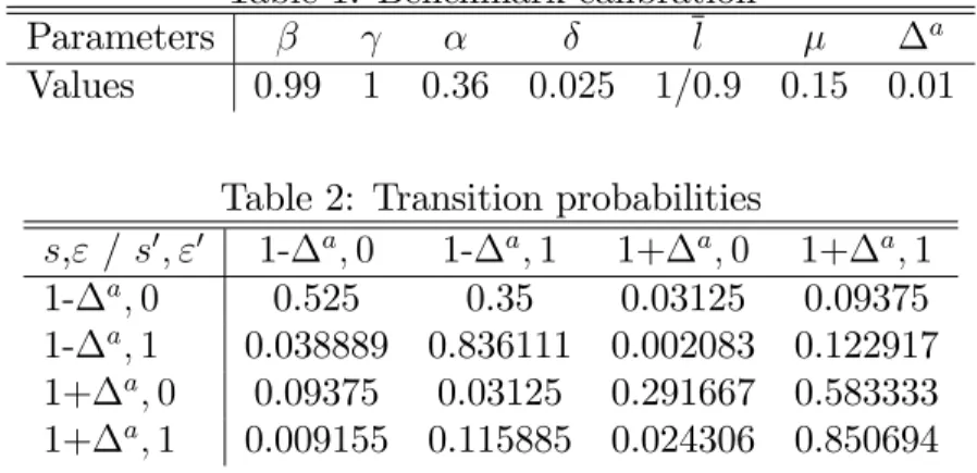
Table 1: Benchmark calibration
Parameters l a
Values 0:99 1 0:36 0:025 1=0:9 0:15 0:01
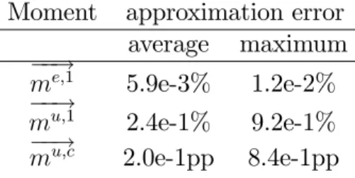
Table 2: Transition probabilities
s," / s0; "0 1- a; 0 1- a; 1 1+ a; 0 1+ a; 1
1- a; 0 0.525 0.35 0.03125 0.09375
1- a; 1 0.038889 0.836111 0.002083 0.122917
1+ a; 0 0.09375 0.03125 0.291667 0.583333
1+ a; 1 0.009155 0.115885 0.024306 0.850694
6.2
Aggregate policy function
In this section, we address the accuracy of the aggregate policy function. In Section 6.2.1, we establish the accuracy of the functional form taking the parameterization of the cross-sectional distribution as given. In Section 6.2.2, we establish whether more moments are needed as state variables. In Section 6.2.3, we describe a more demanding accuracy test by taking a multi-period perspective.
6.2.1 Accuracy of functional form of aggregate policy function
The aggregate policy functions, !e
n(a; a 1; m; e n ) and !u n(a; a 1; m; u n ) capture
the law of motion of the end-of-period values of the three moments that are used as state variables. The approximation uses a tensor product polynomial with at most …rst-order terms for a and a 1, since a can take on only two values, and up to
second-order terms for the elements of m.
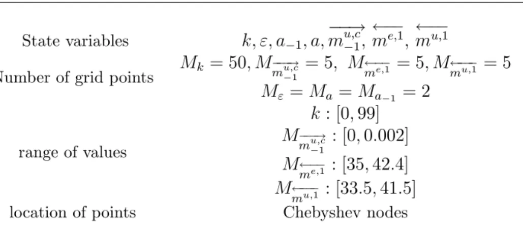
Accuracy is evaluated using a grid of the aggregate state variables on which the three variables with continuous support can take on a …ne range of values. In par-ticular, fme;1g = f35; 35:2; :::; 42:4g, fmu;1g = f33:5; 33:7; :::; 41:5g, and fm!u;c1g = f0; 0:05%; :::; 0:2%g: At each grid point, we use the values of m and the reference moments to obtain the corresponding density exactly as they are calculated in the algorithm. Whether this parameterization of the cross-sectional distribution is ac-curate will be discussed below. Using the parameterized density and the individual policy function, we calculatem!u;c,m!e;1, andm!u;1:These explicitly calculated values
are compared with those generated by the approximations !e(s) and !u(s).
% error across this …ne set of grid points.18 The errors for the …rst-order moment
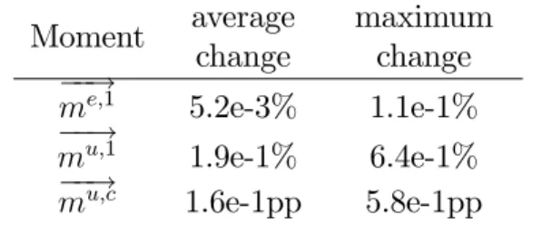
of the capital stock of the employed are small. The maximum error is 0.012% and the average error is 0.0059%. The moments for the unemployed are somewhat bigger, but still relatively small. In particular, the maximum error for the …rst-order moment is equal to 0.92% and the average error is equal to 0.24%. This maximum is attained when the value of me;1 takes on the highest and mu;1 the lowest grid
value, which is an unlikely if not impossible combination to occur. The average and maximum error form!u;c are 0.2 and 0.84 percentage points (pp), respectively.19
There are two reasons why these two numbers are not problematic. First, given that both the actual and the approximation predict very low fractions of agents at the constraint, these errors are of no importance and it wouldn’t make sense to spend computing time on improving the part of !u(s) that determines m!u;c. Second, in
Section 6.2.3, we show using a simulation that the economy doesn’t get close to points in the state space where such large errors are observed. In fact, using a simulation of 1,000 periods we …nd an average error of 0.0076 percentage points and a maximum error of 0.071 percentage points.
Table 3: Accuracy of functional form of aggregate policy function
Moment approximation error
average maximum
!
me;1 5.9e-3% 1.2e-2%
!
mu;1 2.4e-1% 9.2e-1%
!
mu;c 2.0e-1pp 8.4e-1pp
6.2.2 Number of moments as state variables
The algorithm uses m!u;c1, me;1, and mu;1 as state variables and in this section we
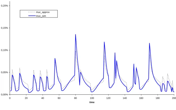
analyze whether additional moments should be used as state variables. That is, conditional on staying within the class of cross-sectional distributions pinned down by the reference moments does it make a di¤erence if additional moments are used as state variables. In particular, we check whether changes in the second-order moment
18Sincemu;c!is a small number and already a percentage, we express the error formu;c!in terms
of percentage points di¤erence an not as a percentage.
19This maximum di¤erence for mu;c! is also attained at the unlikely combination of a very high
value forme;1 and very low value formu;1. At this grid point, the value from our approximation
matter for the key set of moments the agents predict, i.e., m!u;c1, me;1, and mu;1. To
do this we calculate at each of the aggregate grid points m!u;c, m!e;1, and m!u;1 in two di¤erent ways. First, when me;2 and mu;2 take on its reference values, i.e., the average observed in the simulated series (conditional on the value of a). Second, when me;2 and mu;2 take on the maximum values observed in the simulation, but
the values of me;j, and mu;j for j > 2 are still equal to the reference moments.
Table 4 reports for each of the three statistics the average and maximum absolute % change across the grid points when the variance increases.
Table 4: E¤ect of increase in variance under reference distribution
Moment average
change
maximum change !
me;1 5.2e-3% 1.1e-1%
!
mu;1 1.9e-1% 6.4e-1%
!
mu;c 1.6e-1pp 5.8e-1pp
The e¤ect of the increase in the variance on m!e;1 and m!u;1 is small, especially considering that the increase in the variance is enormous. Again, the largest changes occur at unlikely grid points and the changes form!u;c are larger. Of course, it is not
surprising that an increase in the variance has an e¤ect on the fraction of agents choosing a zero capital stock, since the increase in the variance increases the fraction of agents close to zero. Given the lack of importance of agents at the constraint, it doesn’t make sense to add the second-order moment as a state variable.
6.2.3 Multi-period perspective
A word of caution is warranted in drawing conclusions about accuracy from the type of one-period tests performed in the last two sections. The reason is that small errors can accumulate over time if they do not average out. To investigate this issue we compare values form!e;1,m!u;1, andm!u;c generated by two di¤erent procedures. First,
we generate these statistics with our simulation procedure that explicitly integrates over the choices made by the agents in the economy. This procedure does not use our approximations!e(a; a
1; m)and !u(a; a 1; m). Second, we generate these statistics
using only our approximations !e(a; a
1; m) and !u(a; a 1; m). It is important to
point out that this second procedure only uses !e(a; a
1; m) and !u(a; a 1; m), and
38 39 39 40 40 41 41 0 20 40 60 80 100 120 140 160 180 200 time me1_approx me1_sim
Figure 1: m!e;1 generated using the approximation !e(s) or the simulation on a continuum of agents
of motion will be used as the input in the next period.20 This comparison, thus, is
truly a multi-period accuracy test.
The results for m!e;1, m!u;1, and m!u;c are plotted in Figures 1, 2, and 3 respec-tively. The graphs make clear that our approximate aggregate laws of motion do a magni…cent job of tracking the movements of m!e;1 and m!u;1. In fact, one cannot
even distinguish the moments generated by!e(s)and !u(s) from the corresponding
moments generated by explicit integration over the individual policy rules. Some di¤erences between the two procedures are visible for m!u;c, but our approximate aggregate laws of motion track the changes in m!u;c well. As mentioned above, in
a sample of 1,000 observations the average and maximum absolute di¤erence are 0.0076 and 0.071 percentage points, respectively.
6.3
The parameterized cross-sectional distribution
Parameterization of the cross-sectional distribution with a ‡exible functional form serves two objectives in our algorithm. First, it enables the algorithm to calculate
34 34 35 35 36 36 37 37 38 38 0 20 40 60 80 100 120 140 160 180 200 time mu1_approx mu1_sim
Figure 2: m!u;1 generated using the approximation !u(s) or the simulation on a
0,00% 0,05% 0,10% 0,15% 0,20% 0 20 40 60 80 100 120 140 160 180 200 time muc_approx muc_sim
Figure 3: m!u;c generated using the approximation !u;c(s) or the simulation on a
the aggregate laws of motion, !e(s)and !u(s), with standard projection techniques,
since with a parameterized density (i) next period’s moments can be calculated on a prespeci…ed grid and (ii) next period’s moments can be calculated with quadrature instead of the less e¢ cient Monte Carlo techniques. Second, it makes it possible to simulate the economy without cross-sectional variation, which improves the proce-dure to …nd the reference moments.
An accurate representation of the cross-sectional distribution may not be neces-sary for an accurate solution of the model. What is needed for an accurate solution of the model are accurate aggregate laws of motion,!e(s)and !u(s), since the agent
is only interested in predicting future prices and to determine these one does not need the complete distribution, just the set of statistics that determine prices, that is, m!u;c1, me;1, and mu;1.
In this section, we take on the more demanding test to check whether the cross-sectional parametrization, P (k; e) and P (k; u), are accurate. This is a more
de-manding test for the following reasons. First, it requires that all NM moments used to pin down the distribution are accurately calculated instead of just the NM
moments that are used as state variables. More importantly, because the shape of the cross-sectional distribution is endogenous and time-varying, the functional form used must be ‡exible enough to capture the unknown and changing shapes.
To check the accuracy of our simulation procedure and, thus, the accuracy of our parameterized densities, we do the following. We start in Section 6.3.1 with a comparison between the simulated time path of moments generated by our parame-terized densities, with those generated by a standard simulation using NN agents.
The alternative simulation is, of course, subject to sampling variation, but the ad-vantage of the standard simulation procedure is that there is no functional restriction on the cross-sectional distribution at all.
A second accuracy test consists of checking whether the results settle down if NM increases. This is done in Section 6.3.2. The last accuracy test checks whether moments of order higher than NM are calculated precisely.
6.3.1 Comparison between simulation procedures
In this section, we compare the moments generated by our new simulation approach with those generated by the standard Monte Carlo simulation procedure. We re-port Monte Carlo simulations with 10,000 agents and 100,000 agents.21 The same 21In our implementation of the simulation procedure we impose— as in Krusell and Smith
(1998)— that ut = ug (ub) when at = ag (ab). We also ensure that the ‡ows into and out of
(un)employment expressed as a fraction of the total population correspond to those one would …nd with a continuum of agents. Our alternative simulation procedure uses a continuum of agents and
individual policy function is used under the two approaches. We plot time paths of generated moments when we impose the value of a to alternate deterministically between 1 a and 1 + a every 100 periods so that the behavior of the economy
during a transition between regimes becomes clear. A set of initial observations is discarded so that e¤ects of the initial distribution are no longer present.22
Figure 4 reports the evolution of the end-of-period …rst moment of the employed !
me;1. Note that the group of the employed is at least 9,000 (90,000) in the Monte
Carlo simulations with 10,000 agents (100,000 agents). Although the sampling varia-tion is still visible in the graph with 10,000 agents, it is small relative to the observed changes in the calculated moment. It has virtually disappeared in the simulation with 100,000 agents.
Figures 5 shows the evolution of the-end-of period …rst-order moment of the unemployed m!u;1 . The number of observations in this group is much smaller,
amounting to 400 agents (4,000 agents) during recessions in the Monte Carlo sim-ulation with 10,000 (100,000) agents. The sampling variation is substantial in the simulation with 10,000 agents and is still visible in the simulation with 100,000 agents.
The e¤ect of sampling variation is very clear when we consider the fraction of agents at the constraint m!u;c, whose evolution is reported in Figure 6. In this case, even the Monte Carlo simulation with 100,000 agents displays severe sampling variation. The fraction of agents at the constraint is small, and the unemployed do not own much capital. Any inaccuracy due to the high sampling variation is, thus, likely to be inconsequential for the properties of any aggregate series.23
A good way to document the higher accuracy of the new simulation procedure is to look at the transition from the bad regime (high unemployment rate) to the good regime (low unemployment rate). The new simulation procedure clearly shows a sharp increase in the fraction of agents at the constraint when the economy enters the good regime. In contrast, for the standard simulation procedure this increase is not always present and there are many other spikes. The true solution of the model should exhibit such a spike. In this economy, employed agents become unemployed every period. When the economy moves from the high-unemployment to the low-unemployment regime, then the ‡ow out of employment into low-unemployment drops sharply. This means that after the regime change, a smaller fraction of employed automatically imposes the correct stocks and ‡ows.
22Details about the simulation procedure are given in Table 9.
23In this model with only two discrete possibilities for the employment status one could
34 35 36 37 38 39 40 41 42 43 1 51 101 151 201 251 301 351 401 451 501 Time
me1 Non-random cross-section me1 Monte Carlo simulation N=10,000 me1 Monte Carlo simulation N=100,000
Figure 4: m!e;1 generated using a …nite and a continuum of agents
29 31 33 35 37 39 41 43 1 51 101 151 201 251 301 351 401 451 501 Time
mu1 Non-random cross section mu1 monte Carlo simulation 10,000 mu1 monte Carlo simulation 100,000
0,00% 0,25% 0,50% 0,75% 1,00% 1 51 101 151 201 251 301 351 401 451 501 Time
muc Non-random cross-section muc monte Carlo simulation 10,000 muc monte Carlo simulation 100,000
Figure 6: m!u;c generated using a …nite and a continuul of agents
becomes unemployed every period, and thus an unemployed agent is much less likely to have been employed the previous period. Consequently, after a change to the low-unemployment regime, a larger fraction of low-unemployment agents will have a zero capital stock.
To conclude, our new simulation procedure clearly is more accurate than stan-dard Monte Carlo simulation procedures. However, for the current model the sim-ulation procedure is accurate where it matters, namely in tracing the mean capital stock of the employed.
Eventually, not only our proposed simulation method is more accurate than Monte Carlo simulation, but it is also an order of magnitude faster. For instance, Monte Carlo simulations over 3500 periods would take 1 hour and 6 minutes with 10,000 agents and seven hours and 40 minutes with 100,000 agents. In contrast, our simulation procedure takes only 7 minutes for the same number of periods. 24
6.3.2 Increasing NM
In this paper, we use NM moments to characterize the cross-sectional distribution and NM of these are state variables. In Section 6.2.2, we analyzed whether additional
moments are necessary as state variable. Here we address the question whether increasing NM makes a di¤erence.
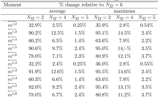
To check the importance of NM, we simulate an economy using di¤erent values of NM to parameterize the cross section. We check when the results settle down. The idea of the test is made clear in Figures ?? and ?? that plot the second and sixth-order moment of the distribution for the unemployed for di¤erent values of NM. The …gures make clear that NM has to be su¢ ciently high. When we increase NM from 2 to 4 then the generated moments change enormously. A further increase from 4 to 5 still causes some changes, but when we increase NM from 5 to 6 then the changes are very minor.
Table 5 reports the results for all moments. It corroborates the results from the …gures. Using a value of NM equal to 2 is clearly way too low to generate an accurate set of moments. An increase in NM from 5 to 6, however, only causes minor changes in the generated moments. For example, the average change for me;2 is only 0.25%
and the average change for mu;2 is equally small. The average (maximum) change for me;6 and mu;6 are equal to 2.3% (3.7%) and 2.4% (3.7%), respectively. These are, thus, somewhat, higher, but as made clear in the graph, these errors are low relative to the observed variation in the moments.
Table 5: The e¤ect of increasing NM
Moment % change relative to NM = 6
average maximum NM = 2 NM = 4 NM = 5 NM = 2 NM = 4 NM = 5 me;2 32.9% 2.5% 0.25% 35.9% 2.8% 0.54% me;3 90.2% 12.5% 1.5% 95.1% 14.5% 2.4% me;4 60.2% 6.5% 1.4% 63.6% 7.9% 2.2% me;5 90.6% 9.7% 2.4% 95.0% 14/-% 3.5% me;6 78.0% 7.1% 2.3% 80.9% 12.1% 3.7% mu;2 32.2% 2.4% 0.25% 36.0% 2.8% 0.55% mu;3 91.9% 12.6% 1.5% 95.5% 14.6% 2.4% mu;4 60.3% 6.6% 1.4% 63.6% 7.9% 2.2% mu;5 92.0% 9.2% 2.4% 95.4% 13.1% 3.5% mu;6 78.0% 6.7% 2.4% 80.8% 11.2% 3.7%
6.3.3 The shape of the distribution
There are two aspects to our approximation of the cross-sectional distribution. First, the class of functions used and second the value of NM. The coe¢ cients are chosen so that the …rst NM moments are correct. But higher-order moments are implied by
the values of the …rst NM moments and the class of functions chosen. For example, when one uses a normal distribution, then one can impose any mean and variance, but skewness and kurtosis are no free parameters.
So for any …nite value of NM, the class of approximating polynomials used, thus, imposes certain restrictions on the function form. Here we check those restrictions along a simulated time path by comparing the jth-order moments for j > NM
implied by the parameterized cross-section with those calculated by integration of the individual’s policy function.
In particular, we do the following. Draw a long time series for the aggregate productivity shock, a. Let e
1 and w1 be the parameters of the cross-sectional
dis-tribution in the …rst period and let me;c1 and mu;c1 be the fraction of employed and unemployed agents with zero capital holdings at the beginning of the period. With this information, we calculate the end-of-period values of the …rst NM moments.25
! mw;11 = 1 Z 0 k("w; k; s) P (k; w1)dk; w 2 fe; ug: (16) ! mw;j1 = 1 Z 0 k("w; k; s) mw;11! j P (k; w1)dk; 1 < j NM; w2 fe; ug: (17)
In exactly the same way, we calculate higher-order moments. That is, ! mw;j1 = 1 Z 0 k("w; k; s) mw;11! j P (k; w1)dk; j > NM; w2 fe; ug: (18)
Now we check whether these higher-order moments (j > NM) are similar to the mo-ments implied by the parameterized cross-sectional distribution. To do this, we use the …rst NM end-of-period moments to calculate the coe¢ cients of the corresponding 25By indicating in bold the variable that we are integrating over, we make clear that we are
approximating density,!e
1 and!u1. Next, we calculate higher-order moments implied
by this parameterized cross-sectional density. That is, ! =j1 = 1 Z 0 k mw;11! j P (k;!w1)dk; j > NM; w 2 fe; ug: (19)
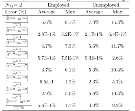
If the shape of the cross-sectional distribution is not too restrictive, then the implied higher-order moments correspond to the explicitly calculated higher-order moments. We perform this exercise using values for NM equal to 2 and 6 and then calculate the average and maximum error observed along the simulation of 2,000 observations with the error term de…ned as follows:26
=w;n mw;n
mw;n :
Table 6: Implied and actual higher-order moments; NM = 2
NM= 2 Employed Unemployed
Error (%) Average Max Average Max
=w;3 mw;3
mw;3 5.6% 9.1% 7.0% 15.3%
=w;4 mw;4
mw;4 2.8E-1% 3.2E-1% 2.1E-1% 6.4E-1%
=w;5 mw;5
mw;5 4.7% 7.5% 5.6% 11.7%
=w;6 mw;6
mw;6 5.7E-1% 7.5E-1% 9.3E-1% 2.6%
=w;7 mw;7 mw;7 3.7% 6.1% 5.3% 10.3% =w;8 mw;8 mw;8 6.5E-1 1.2% 2.3% 5.7% =w;9 mw;9 mw;9 2.9% 5.0% 5.6% 10.3% =w;10 mw;10 mw;10 5.6E-1% 1.7% 4.0% 9.2%
26Note that the accuracy measure is actually de…ned for beginning-of-period moments, but this
is simply a transformation of end-of-period values taking into consideration the change in the employment status.
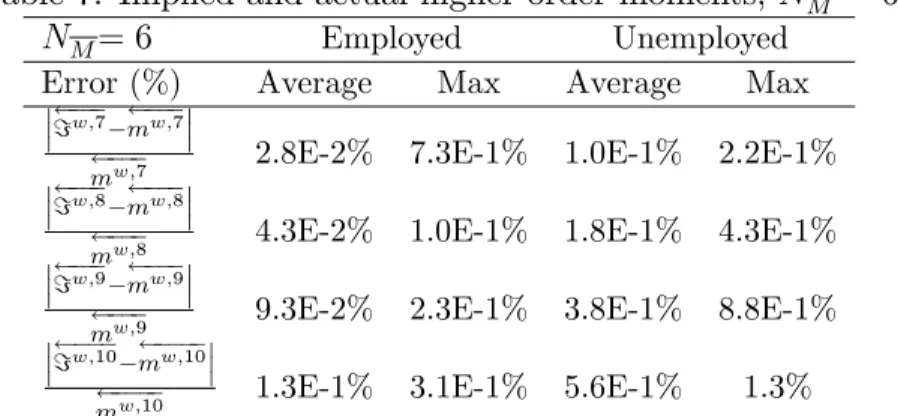
Table 7: Implied and actual higher-order moments; NM = 6
NM= 6 Employed Unemployed
Error (%) Average Max Average Max
=w;7 mw;7
mw;7 2.8E-2% 7.3E-1% 1.0E-1% 2.2E-1%
=w;8 mw;8
mw;8 4.3E-2% 1.0E-1% 1.8E-1% 4.3E-1%
=w;9 mw;9
mw;9 9.3E-2% 2.3E-1% 3.8E-1% 8.8E-1%
=w;10 mw;10
mw;10 1.3E-1% 3.1E-1% 5.6E-1% 1.3%
Tables 6 and 7 report the errors for NM = 2 and NM = 6; respectively. When NM is equal to 2, then observed error terms are large for the odd-numbered mo-ments. That is, the shape of the distribution implied by our class of approximating functions doesn’t capture the correct shape of the distribution when a second-order approximation is used. The results are much better when NM is equal to 6. Now we
observe much smaller errors. The largest errors are for the 10-th order moment of the capital stock of the unemployed. For this moment, the maximum error is 1.3%, which is not excessively high.
7
Concluding comments
In this paper, we have developed a new algorithm to solve models with heteroge-neous agents and aggregate uncertainty. We used the algorithm to solve the model in Krusell and Smith (1998) and found our numerical solution to have similar prop-erties to the one obtained with simulation procedures. The ability to obtain similar numerical outcomes with quite di¤erent algorithms builds con…dence in the results. Accuracy tests, of course, can do the same but they also have its limits, especially in high-dimensional models.27 The models the profession will consider in the future are
likely to become more complex. Since di¤erent algorithms have di¤erent strenghts and weaknesses it is important to have a variety of algortithms to choose from. This paper helps to create a richer portfolio of algorithms to solve these complex models especially because the building blocks used are so di¤erent from the popular alternative.
27In particular, small errors that accumulate over time to non-trivial magnitudes may be hard
A
Appendix
A.1
Details on Transition equations
This appendix describes how the change in employment status that occurs at the beginning of each period a¤ects the moments of the cross-sectional distribution. Al-though, we use centralized moments as state variables, we actually do not use cen-tralized moments here. It is easier to …rst do the transformation for non-cencen-tralized moments and then calculate the centralized moments.
From beginning to end-of-period. Let ga;w be the mass of agents with
employ-ment status w when the economy is in regime a. At the beginning of the period we have to following groups of agents:
1. Unemployed with k = 0, whose mass is equal to mu;cg a;u
2. Unemployed with k > 0, whose mass is equal to 1 mu;c g a;u
3. Employed with k = 0, whose mass is equal tome;cga;e
4. Employed with k > 0, whose mass is equal to 1 me;c ga;e
Agents in group #1 choose k0 = 0, while agents in group #2 either set k0 = 0
or k0 > 0. Let the fraction of agents that set k0 = 0 be equal to k0=0
u;k>0. Thus, the
fraction of unemployed agents that set k0 = 0, is equal to
!
mu;c =mu;c+ ku;k>00=0 (1 mu;c):
The ith moment of the capital stock chosen by agents in group #2 is equal to
k0 0;i u;k>0 = k0=0 u;k>0 0 i + (1 ku;k>00=0 ) m!u;i: Thus, ! mu;i = k0 0;i u;k>0 (1 ku;k>00=0 ) where ku;k>00 0;i =R0+1k(0; k; s)iP (k; u)dk.
!
me;c = 0, since employed agents never choose a zero capital stock. To calculate
!
k0>0;i
e;k=0 = k(1; 0; s) i
;
and the mean of the capital stock chosen by those in group 4, i.e.,
k0>0;i
e;k>0 =
Z +1
0
k(e; k; s)iP (k; e)dk:
Weighting the two means gives ! me;i= m e;c k0>0;i e;k=0 + (1 me;c) k0>0;i e;k>0 me;c+ (1 me;c)
From end-of-period to beginning of next period. At the end of the current
period, we have to following groups of agents:
1. Unemployed with k0 = 0, whose mass is equal to m!u;cg a;u
2. Unemployed with k0 > 0, whose mass is equal to (1 m!u;c)ga;u
3. Employed with k0 > 0, whose mass is equal to g a;e
gww0;aa0 stands the mass of agents with employment status w that have
employ-ment status w0 in the next period period, conditional on the values of a and a0. For
all combinations of a and a0 we have,
guu;aa0 + geu;aa0 + gue;aa0 + gee;aa0 = 1:
The number of agents with k0 = 0as a fraction of all agents that are unemployed
in the following period is equal to
mu;c0= guu;aa0 guu;aa0 + geu;aa0
! mu;c:
and the fraction of all employed agents at the constraint is equal to me;c0= gue;aa0
gue;aa0 + gee;aa0
! mu;c
Next period’s ith-order moments of the distributions with strictly positive capital