Can polyethylene passive samplers be used to measure infiltration?

Can Polyethylene Passive Samplers be Used to

Measure Infiltration?

by

Tanguy Raguenez

Submitted to the Department of Civil and Environmental Engineering

in partial fulfillment of the requirements for the degree of

Master of Engineering in Civil and Environmental Engineering

at the

MASSACHUSETTS INSTITUTE OF TECHNOLOGY

June 2017

@

Massachusetts Institute of Technology 2017. All rights reserved.

Signature redacted

A uthor ...

...

Department of/ivil and Environmental Engineering

May 12, 2017

Certified by...Signature

redacted...

Eric Adams

Senior Research Engineer and Senior Lecturer

Thesis Supervisor

Signature redacted

Accepted by ...

...

I

_{Jesse Kroll}

MASSACHUSTS INSTITUTE

Professor of ivil and Environmental Engineering

OF TECHNOLOGY

vlanEgierg

Chair, Graduate Program Committee

JUN 14 2017

LIBRARIES

-Can Polyethylene Passive Samplers be Used to Measure

Infiltration?

by

Tanguy Raguenez

Submitted to the Department of Civil and Environmental Engineering on May 12, 2017, in partial fulfillment of the

requirements for the degree of

Master of Engineering in Civil and Environmental Engineering

Abstract

Environmental impact assessments on contaminated sites require to understand all of the possible sources of pollution in the field, including groundwater seepage. Polyethy-lene passive samplers have been used extensively to measure a chemical's concentra-tion in the sediment or water column and convenconcentra-tional seepage meters are deployed to infer the infiltration flux. A model was developed to describe how passive samplers could instead realize both these functions to completely characterize contamination through seepage in the environment. The simulations describe the concentrations in a strip of polyethylene inserted in sediment where porewater flows steadily and vertically. Providing that the target chemical's diffusion and partitioning properties in the sediment are known, the model allows the user to obtain concentration profiles in the passive sampler at different infiltration velocities. Experimental data can then be fitted on these profiles to deduce infiltration within a factor of 2. The approach is promising and was successfully tested in the laboratory using naphthalene, and fur-ther studies should be made to fully validate the use of passive samplers as seepage meters.

Thesis Supervisor: Eric Adams

Acknowledgments

I would like to thank the United States Geological Survey (USGS) and in particular Denis Leblanc for providing seepage meters and assisting the project during a field study in Ashumet Pond. I would also like to thank my advisor Dr Eric Adams for his guidance during the year, as well as Pr Philip Gschwend for his assistance in the preparation of the experimental measurements presented in this paper.

Contents

1 Introduction

2 Passive Samplers: General Concepts

2.1 Underlying Theory of Concentration Measurements . . . . 2.1.1 Performance Reference Compounds . . . . 2.1.2 Partitioning and Equilibrium Models . . . . 2.2 Protocol and Measurement Method of PE Passive Samplers .

2.2.1 Preparation and Testing of PE strips . . . . 2.2.2 Sediment Sampling Methods . . . .

2.2.3 Extraction and Analyses of Pore Water and Polyethylene

3 Existing Seepage Measurement Methods: why study samplers?

3.1 Conventional seepage meters ... 3.2 Other seepage measurement methods ...

3.2.1 Heat tracer methods . . . . 3.2.2 Using Darcy's Law . . . . 4 Modeling of PE Passive Samplers in Infiltration Zones 4.1 Theoretical M odel . . . . 4.1.1 2-D Geometry of the Problem . . . . 4.1.2 Input Parameters . . . . 4.1.3 Governing Equations . . . . PE passive 18 . . . . 18 . . . . 20 . . . . 20 . . . . 21 23 . . . . 24 . . . . 24 . . . . 26 . . . . 28 8 10 11 11 12 14 14 15 16

4.1.4 Boundary and Initial Conditions . . . . 4.2 Numerical Model . . . . 4.2.1 Spatial and temporal discretization . . . . 4.2.2 Coefficient Matrices . . . . 4.2.3 Precision and Stability of the Model . . . . . 5 Numerical Simulation Results and Analysis

5.1 Observing concentration over time . . . . 5.1.1 Presentation and Purpose . . . ... 5.1.2 Results and Analysis . . . . 5.2 Observing concentration at different infiltration rates

5.2.1 Presentation and Purpose . . . .

5.2.2 Results and Analysis . . . . 6 Ex situ Validation of Numerical Model

6.1 Description of the Experiments . . . .

6.1.1 Main Setup . . . .

6.1.2 Measurement Method . . . . .

6.2 Results and Analysis . . . . 6.2.1 Experimental Results . . . . 6.2.2 Validating the Model . . . . 7 Conclusions and Next Steps

A Matlab Code 28 29 30 32 35 36 36 36 37 40 40 40 45 . . . . 45 . . . . 45 . . . . 47 . . . . 49 . . . . 49 . . . . 50 52 54

Chapter 1

Introduction

Polyethylene (PE) passive samplers are usually deployed to measure' dissolved phase concentrations of hydrophobic organic compounds (HOC) such as PAHs and PCBs in a contaminated environment. They consist of a thin sheet of polyethylene, coated in a reference compound (PRC) and placed in a rigid frame. PE samplers have been used to determine the state of contamination in a water bed, and are key in evaluating the required remediation efforts to reduce the hazards

[9].

Numerous studies have been conducted to characterize how passive samplers mea-sure HOC concentrations

181.

The process relies on partitioning estimates of the compound among the different phases of the sediment. Chapter two introduces the primary underlying concepts of concentration measurements using PE samplers.

HOC contamination in the environment can have multiple sources, such as river and lateral fluxes, resuspension and groundwater infiltration, i.e. seepage, which is our focus. Whereas PE samplers can determine the concentration of pollutants in the sediment, as of now (in their usage) they do not measure the porewater velocity and therefore the flux of HOC from the bed to the water column. Chapter three describes how seepage measurements are made in sediment beds and why these are important to define remediation efforts. Multiple measurement tools are presented and compared. The case of the Lower Duwamish Waterway (LDW) in Washington is studied briefly to explain how cheap, reliable and easy to operate seepage meters are

key in alleviating HOC (in this case PCBs) pollution. The objective is to demonstrate how conceptually, PE samplers can provide an interesting alternative to conventional seepage meters in measuring sediment porewater velocity.

First, this work attempts to compute numerically how PE samplers could measure porewater sediment velocity and what its theoretical sensitivity would be. Chapter 4 presents the diffusion and advection model and the assumptions made. In chapter 5, the numerical simulation results are presented and discussed. These results give a first insight on the feasibility of using PE samplers and partitioning estimates to measure a velocity.

Finally, laboratory experiments calibrated from the numerical results were con-ducted to verify theoretical protocol of using the samplers in seepage measurements. Chapter 6 details the experiments and studies how the results at varying times and varying velocities compare to the numerical model. While further experimental val-idation is required, the results are promising and certainly allow to envision the use of passive samplers as seepage meters.

Chapter 2

Passive Samplers: General Concepts

In this section, the underlying concepts of polyethylene passive samplers, the theoret-ical model and protocol of the concentration measurements, are presented. Various polymeric passive samplers have been deployed to assess hydrophobic organic chemical contamination in the environment, but this paper focuses on the use of Performance Reference Compounds (PRC) in the samplers to deduce the chemical concentrations. These samplers have been developed extensively at MIT in the Ralph M. Parsons Laboratory since 2009

[4][?]nonpolar,

and offer an improved contamination risk as-sessment from regular polymer-based samplers.

The PE passive samplers consist of a strip of polyethylene fixed in a steel frame designed to be inserted in the sediment bed. The preparation of the PE strip will be discussed in greater detail later in the chapter. The following picture shows a PE passive sampler as it is developed at MIT.

Figure 1: A Polyethylene Passive Sampler being prepared in the MIT laboratory.

This chapter first illustrates the underlying models for the samplers, in particular how the equilibrium HOC concentration can be deduced from the chemical uptake in the sampler. Then, this chapter reviews the measurement method and how the PE samplers operate in the field.

2.1

Underlying Theory of Concentration

Measure-ments

2.1.1

Performance Reference Compounds

The general concept behind polymer-based passive samplers is that by inserting the polymer strip inserted in the environment (water, sediment, etc.) contaminants will sorb to the polymer and once equilibrium is reached, the concentration in the poly-mer reflects the concentration in the environment. Use of Performance Reference Compounds (PRC) in samplers is motivated by two main defaults of most regular polymeric samplers: requirements to take samples for equilibration in a laboratory and the long equilibration time when experiment conducted in situ [8].

The first passive samplers were designed to measure freely dissolved water concen-trations of chemicals using equilibrium concenconcen-trations

14].

The HOC would accumu-late in the polymer proportionally to the environment concentration, a process which can be very slow. However, use of PRCs, previously impregnated in the PE, allows to measure concentrations before equilibrium is reached [13J. There are different meth-ods to extrapolate the equilibrium concentrations at a time t before equilibration.

First, if the mass transfer rate of the PRC and the HOC in and out of the PE strip are the same, the HOC concentration in the environment is simply [8]:

C* - CHOC(t)CPRC,init

C PRC,init - CPRC(t)

With CHoc(t) the concentration of HOC measured in the polymer at the time t,

CPRC,init the initial PRC concentration in the polymer and CPRC (t) the concentration of PRC remaining in the polymer at the time t. However, this is only likely if mass transport is controlled by diffusion through the polyethylene, which is not often the case with HOCs, for which transport is often controlled by diffusion through the sediment or the water. In this case, the PRC and target HOC may behave differently in the sediment, in particular regarding sorption to the solid particles (mineral or biological) present in the environment. PRCs are still used to extrapolate mass transfer rates through the PE but further knowledge of the chemicals' sorption and partitioning properties are required.

2.1.2

Partitioning and Equilibrium Models

Determining the sediment porewater concentrations of a chemical requires knowing its sorption properties. Essentially, the two variables we want to know are Kd, the "normal" sorption coefficient, and KPEW, the polymer-water partition coefficient. As

described by Fernandez et al [8], PRCs can still be used to determine the sorption coefficients of the target chemicals.

Indeed, using at least two PRCs of the same chemical compound class as the target HOC and the relationship between log Kow and log Kd, we can estimate the

sorption coefficient of the target chermical.

Knowing the sorption parameters of the target chemical, what is the partitioning model in the sediment bed? The sorptive capacity of the passive sampler is described

by the following relationship [31:

3

mol KPEW [3 mo

capacity[ - = x L[cmPE X Csedi I

cm

W[

Kd and KPEW are the previously described partitioning coefficients, L is the half thickness of the PE strip, and Ced is the chemical's concentration in the sediment. We can see that only is last parameter, Csed, changes with time and that as the target is depleted around the PE, Csed will locally decrease and the rate of sorption in the strip will also decrease. This explains why the time to reach equilibration in the polymer is often very long. Overall, the time Tsed to reach equilibration in the PE

depends on the studied chemical and the sediment, and is a function of the partition coefficients, L, the tortuosity (T) and porosity (#) of the sediment and the diffusion

coefficient in the water:

KS-Ew x )(2 Tsea = = constant Kd x Dw X 1 105 .0 0.8 * 0.6- ~ S0.4 108 U- 0.2- ₁₀₉ 0 10 30 60 90 120 150 180 240 300 360 Time (days)

Figure 2: Approach to equilibrium for a passive sampler deployed in a stagnant sediment bed over time (in days) for different Tsed (in seconds) values

[3].

The previous plot shows that the greater the equilibration time TSED is, the slower the intake of the chemical is, and the process can take several years. The entire approach of measuring the chemical uptake rates in the PE and correcting the values with measurements of PRC loss (taking into account both organic and black carbon) have been verified and agree with in situ data [4].

2.2

Protocol and Measurement Method of PE

Pas-sive Samplers

In this section, PE passive samplers are presented in a more practical way in an attempt to answer questions such as how they are fabricated and prepared, what is the best way to deploy them and how the measurements are operated. The goal is to understand how easily they can be used on the field to compare them in Chapter 3 with different seepage measurement methods.

2.2.1

Preparation and Testing of PE strips

Preparation

The preparation process of the PE strips is relatively straightforward. The sheets of polyethylene are usually 25 or 100 pm thick and can simply be bought in a hardware store.

First, the PE is impregnated with the desired performance reference compound. After being soaked consecutively twice in dichloromethane, twice in methanol and twice in water, each time for 24 hours, the strip is placed in a solution containing the PRC. In order to achieve a uniform equilibration in the PE, this process can last from a couple of days to several months

[91

depending on the chemical. Then, the polymer sheet is incased in the second piece of the passive sampler: the steel frame, which is constructed to penetrate the sediment and to be easily mounted on a platform.

Testing

in the PE, DPE, and the polyethylene-water partition constant

KPEW-First, by doing various water measurements with the polyethylene for different PAH (polycyclic aromatic hydrocarbons) and PCB compounds, we can estimate the equilibration of these HOCs inside the PE. From this, we can estimate the KPEW

for each of the compounds and an empirical log-linear relationship logKPEW= a X

logKow + b (a and b constants) which we can use for other HOCs with known Kow

values

[9].

Similarly, DPE can be measured for different molar volumes V from which we can extrapolate another log-linear relationship: logDPE = a x V + b

[9].

Finally, further laboratory testing can be made for different sediments and con-ditions to study the passive sampler's behavior in the environment. Parameters like water temperature, flow rate, current, salinity, etc. can be studied in detail (an example of an ex situ testing is described extensively in Chapter 6).

2.2.2

Sediment Sampling Methods

Initially, the sites where the passive samplers are deployed are chosen according to historical information of contamination (ex: knowledge of a previous industrial outfall location) and past measures of HOC concentration. Once the PE strips are attached to their aluminium frame, they need to be inserted at the desired locations from a boat. Indeed, one of the advantage of these passive samplers is that they do not nec-essarily require divers to deploy them. The following picture illustrates schematically two PE samplers in their aluminium frame ready to be lowered into deeper waters from a boat (not represented) [9].

,Adeo camera

Figure 3: PE sampler in an aluminium frame ready to be deployed in deeper water from a boat 191.

The deployment vehicle represented above needs to meet a few criteria (small enough to fit on a boat, resistance to corrosion, have "adjustable" weights, be easy to retrieve, etc) so may need to be built and designed for specific use. Weights can be added or removed depending on the nature of the sediment and the need for extra penetration.

The PE samplers need to be inserted about 10cm into the sediment and the sam-pling time is around a week. These parameters can vary depending on the nature of the sediment and the target HOC (different equilibration times for different com-pounds). Immediately after extraction, the PE samplers are rinsed with clean water and wrapped in aluminium foil. This is to prevent as much as passible the target HOC impregnated in the PE from diffusing in the air. They are sent to the laboratory for testing and to determine the PRCs and target chemicals' concentrations

[91.

2.2.3

Extraction and Analyses of Pore Water and

Polyethy-lene

Different analyses can be made on the polyethylene strip and retrieved sediment and/or organisms (ex: clams) found at the sampling site. Indeed, analyzing in detail the environment at the sites can give greater insight on the target's preferential loca-tions and help understand how organisms react to it. The process of extracting PAHs

and PCBs from sediments and organisms can be tedious and is explained extensively in Gschwend's SERPD Project report [9]. However, in this paper's interests, only the PE is useful for possibly predicting sediment porewater velocity (cf Chapter 4 for further information) so only the PE analysis method will be reviewed.

After being cleaned and rinsed again, the PE strip is cut into sections of about 4cm length. To extract the target chemical and PRC from the strip, the PE is then soaked in dichloromethane for a day, and the extracts are combined and concentrated to be analyzed. This allows greater precision in determining the different compounds' concentrations.

What is the accuracy of this method? Gschwend et al

[9]

conducted experiments to compare the concentration deduced using PE passive samplers and concentrations found using other methods (porewater extraction, sediment extraction, air bridges, etc.). The studies were made with a representatitve PAH and a representative PCB and found that PE passive samplers were accurate to a factor of two or three and had a precision of 30%. Other methods were not as accurate, which proves the interest for using these samplers to measure sediment porewater or fully dissolved concentrations.

Chapter 3

Existing Seepage Measurement

Methods: why study PE passive

samplers?

As previously stated, seepage measurements are a key component of risk assessments in contaminated sites. There are multiple ways to measure groundwater seepage into surface water, from measuring directly the water flux, to using more technical methods such as visualizing temperature gradients with a fiber optic cable [12]. How efficient are each of these methods? What are their advantages and defects? Multiple factors such as spatial and temporal scales, uncertainties, or the nature of the site should be taken into account when choosing a seepage meter.

This chapter aims to illustrate the range of seepage meters, that are most currently used, and how PE passive samplers could be a useful fit among the other meters. This is not an exhaustive list of seepage meters but rather a review of the three prominent methods.

3.1

Conventional seepage meters

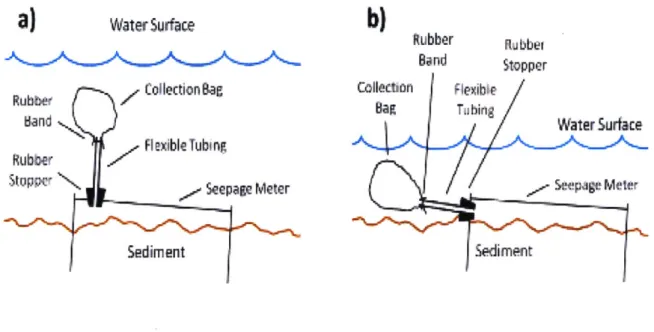
These are the most commonly used seepage meters and operate by making direct water flux measurements on the sediment bed. A sealed "container" (typically the

top of an oil drum) is placed on the bed to enclose a specific area and the amount of water that flows through this area during a time At is collected in a bag at the end of the container. The basic setup is represented in Figure 4

[?]:

a)

WaterSurface

Rubbe Collection Bag

Hand

,,. Flexible Tubing

Stoppcr _{Seepage Meter}

Sediment

b)

Band Stopper Collecion Flexible Water Surt: Lo Sediment

Figure 4: Cross section view of a typical installation of conventional seepage meters (left) and in shallow waters (right).

An initial amount of water V is placed in the collection bag in case the flux is from the water column to the sediment bed. The volume of water V collected after At is measured and we can infer the average seepage

Q

at the chosen cite with a simple relationship:

V

-V

Q At

(It is worth noting

Q

is only a measure of seepage at a given location and at a given time. Groundwater flow can be very dynamic and change a lot with time and space.) Conveniently, when combined with hydraulic head measurements, these meters can estimate the hydraulic conductivity K of the sediments using Darcy's law. Also, these seepage measurements have been proven to be relatively accurate [5]. An error of less than 20% was consistently observed during multiple tank tests. The

preparation and analysis processes are very direct so few external factors can impact the measurement of the flux.

However, while the concept behind these meters is simple, their deployment is not as straightforward. For one, many problems have been observed with the collection bag. As explained by Kalbus et al. [141, water flowing around the bag may distort the bag or affect the hydraulic head in it, which can result in an inaccurate volume at the end. Also, in deeper waters, these meters require the intervention of divers and may need to be checked regularly. Finally, the accuracy of the measurements is greatly impacted by the spatial variability of seepage flux in the sampled area [17I. It is not advised to use these seepage meters in sites where the flux varies a lot within a small area. Therefore, the sampling site needs to be carefully chosen to mitigate this variability as much as possible.

Different variations of this model exist, such as having rigid bags less affected by passing flow, or automated meters that record the flow rate directly at the outlet tube [141. This is done with various instruments, such as electromagnetic meters (voltage induced by and proportional to passing fluid in an electromagnetic field), ultrasonic meters, dye-dilution meters and heat pulse meters.

3.2

Other seepage measurement methods

3.2.1

Heat tracer methods

As stated previously, some automated seepage meters include heat signature mea-surements to infer the water flux. Many different heat tracer methods can be used to measure seepage.

Heat tracer methods use the difference in temperature between groundwater and surface water to identify seepage. Groundwater temperature stays relatively con-stant, whereas surface water changes temperature during the day, with diurnal cycles. Therefore, if in a site sediment water temperature stays constant and surface water has dampened diurnal temperature cycles, this is indicative of water flowing from the

sediment bed at constant temperature and homogenizing surface temperatures. By contrast, losing reaches for surface water can be characterized by variable sediment temperatures [14]. A detailed review of using heat as a tracer, the heat transport equation models in the sediment and water and simulations is presented by Anderson

[1].

This method is popular for detailed mapping of groundwater seepage as temper-ature measurements are relatively inexpensive, immediate and easy to perform. The temperature in the water column or along the sediment bed can be made simply by direct measurements or with a thermal infrared camera. Although they only require a good numerical model and estimate for thermal and hydraulic conductivities in the sediment, a lot of calibration is still needed to obtain valid results.

Moreover, innovative ways to measure temperature exist, such as using fiber optics: this method is called fiber-optic distributed temperature sensing (FO-DTS). A pulse of light is sent in a cable and the returned scatter energy is collected and measured. The cable is extended on the sediment bed and can provide measurements on its entire length (up to 10km long) with a spatial resolution of 1 meter and a temporal resolution of 30 seconds [12]. Simultaneously, a MER cable (marine electrical resistivity) is placed next to the FO-DTS cable and indicates the delimitation of freshwater and saltwater. Indeed, saltwater is more conductive than freshwater and returns a stronger signal. An extensive study by Hare et al. (2015) [11] compares this method to typical measurements with thermal infrared (TIR) cameras. Overall, the FO-DTS method is spatially more precise and detects seepage on the sediment bed better than TIR cameras. However, unlike these cameras, it did not identify seepage that occurred on the banks, which shows why in certain cases, multiple seepage meters should be combined.

3.2.2

Using Darcy's Law

Darcy's Law is used to calculate the specific discharge or Darcy flux q within an aquifer:

dh

q

=-K--dl

K is the hydraulic conductivity and 4 the hydraulic gradient. Methods based on this principle simply aim to estimate these parameters and deduce q.

The hydraulic gradient can simply be measured in wells and piezometers installed in the study sites. However, to establish a gradient, groundwater needs to flow be-tween the sites, which means they are in the same aquifer and that there are no geological obstacles in the way. To measure the sediment's hydraulic conductivity, samples are collected and studied in the laboratory. Conductivity is then measured by analyzing the grain size (first estimate) and making permeameter tests (using Darcy's law). Similarly, the geological nature and hydraulic conductivity needs to be know at each point between the two study sites [14J. K is never homogeneous over an area, which adds further uncertainty. Overall, this method is impractical wherever the sediment geology is heterogenous and previously uncharacterized, which is often the case.

Why is it interesting to study passive samplers as a way to measure seepage? By already determining contaminant concentrations in the environment, the sam-plers could be used to measure contaminant infiltration in the water column in one measurement and with one tool. Secondly, passive samplers are easy to operate and relatively inexpensive, especially compared to FO-DTS measurements. They could be used as a less costly alternative to heat tracer methods and as a complement to conventional seepage meters by both measuring the target concentration and corrob-orating the seepage measurement with their own estimate of it.

Chapter 4

Modeling of PE Passive Samplers in

Infiltration Zones

Now that we have identified how the market of seepage meters is open to new tech-nologies for contamination assessments, we need to characterize how passive samplers can effectively measure infiltration. Indeed, it can be conceptualized that when a sam-pler is placed in sediment and subjected to water flow, the discharge rate of PRCs from the PE will not be the same as if there wasn't any flow, and will evolve if the flow increases, decreases, reverses, etc. How can this be modeled and verified?

Before verifying with practical experiments in the laboratory or in the field if PE samplers can measure seepage, it is essential to model and predict the sampler's behavior beforehand. For one, if the models predict samplers cannot measure infiltra-tion, for instance if the concentrations observed at high and low seepage are minimally different, then it is not necessary to conduct any further experiments. Moreover, these models can provide a basis and curves on which in situ and ex situ data points could be fitted. This chapter focuses on the physical model used for the simulations and details the numerical model which is tested in Chapter 5.

In our model, the PE is initially impregnated with a chemical, not present in the environment, and we simulate how the concentrations in the PE and in the sediment evolve with time and infiltration.

4.1

Theoretical Model

4.1.1

2-D Geometry of the Problem

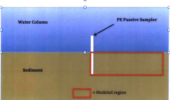
The passive sampler and the environment are modeled in this paper in two dimen-sions. It is a more simple first approach and we can consider that the thickness of the polyethylene strip (100pm) is much smaller than its width (about 10cm) so the chemicals will essentially diffuse into the environment through the PE's thickness. The following diagram illustrates the 2D situation where a passive sampler is intro-duced in the sediment bed of a water column. The cross section visualizes the height and thickness of the passive sampler.

PE Passive Sampler

Water Colum

Modeled region

Figure 5: Cross section diagram of a passive sampler introduced in the sediment bed of a water column. The width of the sampler is normal to the page.

The red rectangle represents the specific section we will model numerically. This paper focuses on use of PE samplers to measure infiltration and therefore our goal is to measure the porewater velocity w in the sediment. Near the sediment-water interface, this velocity w should be vertical. Figure 6 is a closer view on the analyzed portion of the sediment and polyethylene.

z

PE

SED

h

L

Figure 6: Cross section diagram of a passive sampler introduced in the sediment bed of a water column.

The diffusion and advection problem is symmetrical so we can restrict the analysis to half the thickness of the polyethylene. The white rectangle represents the passive sampler (denoted PE); h is the depth of the sampler in the sediment (note that the total length of the sampler is greater than h, as part of the PE sticks out in the water column) and is around 10 cm depending on how deep the sampler can be inserted, and I is the half-thickness of the PE, around 50 pm. The brown rectangle represents the sediment (denoted SED); h is the height of the sediment in our model (above is the water column and below we consider there is no repercussion on the PE), and L is the length of sediment in our study. Theoretically, L is infinite but as we will see in the next chapter displaying our results, we only need to have L around 1 meter to be considered infinitely far from the passive sampler.

The x dimension is along the thickness and the dimension in z is vertical.

4.1.2

Input Parameters

Concentrations

The PE is initially impregnated with a performance reference compound. The nature of the PRC is not important to our problem, but we suppose that it is not present initially in the environment. The concentrations of the PRC are the param-eters we want to measure and control in the problem - they are the main variables.

CPE(X, z, t), a function of time and space, is the concentration of the chemical in the

polyethylene. Similarly, CSED(X, z, t) represents the concentration of the chemical in the sediment porewater. Indeed, the chemical in the sediment can be present in the water, the solid particles or biological organisms but we consider it essentially moves in space only in the water phase. However, the sorption component in the sediment is taken into account with the diffusion coefficients and partitioning constants.

Partition Coefficients

The partition coefficients describe the equilibrated concentrations of a chemical when multiple phases are present. In particular, in our model, the PRC can be present in the polyethylene, in the porewater and in the solid sediment particles. This simplified approach does not consider sorption to biological mater and considers the sediment to be of uniform nature. We can therefore define the following partition coefficients (all concentrations are at equilibrium):

KPE -CPE cm 3 ~ae

Cw _{lcm3 pol ymer.}

_Cry sed 1 [cm

3 _water

Cw Psed cm3 sed

KPEW is the polymer-water partition coefficient and Kd is the sediment-water partition coefficient (the sediment density introduced to have matching cm3 _units,

the "classic" sorption coefficient with sediment has units of "3

water

).

Finally, we can

g dry sed a

define the polymer-sediment partition coefficient KPESED:

KPEW cm3 sed1

KPESED ~ K _[cm3

PE_

Diffusion Coefficients

Movement of the chemical in the environment is partly controlled by diffusion processes, which are considered to be Fickian. The molecular diffusion coefficient in the porewater, D, is approximately 10--cm2_{/s and the molecular diffusion coefficient}

in the polyethylene, DPE is in the order of 3 x 10-10 cm2_{/s. Finally, the molecular}

diffusion coefficient in the sediment (porewater + solid particles) can be expressed with D., Kd, the tortuosity T and the volume ratio of solid particles to water calcu-lated from the porosity r,, and reflects diffusion through the porewater retarded by sorption to solid particles [8]:

DSED - ( D)

(I + r,,,Kd )T

Sediment Porewater velocity

In our simplified model, w, the sediment porewater velocity, is both constant and uniform. We consider that w is uniformly vertical to characterize a uniform water flux in or out of the sediment. It is also worth noting that although w is represented as positive in Figure 6, the seepage is from the sediment to the water column, it can also be reversed (negative sign) to model seepage from the water column to the bed. Whilst the velocity is uniform and constant for one simulation, it can obviously be changed between simulations. During a field trip to Ashumet pond in Cape Cod, infiltration velocity measurements made with conventional seepage meters indicated that in the environment, sediment porewater velocity is of the order of 1-10 cm/day. During our simulation and ex situ experiments, w will be of this order of magnitude and vary from around 1 to 20 cm/day.

4.1.3

Governing Equations

The concentrations in the polymer and sediment are characterized by a transport equation. We make the following assumptions in our model:

(1) There are no external sources or sinks (conservative compound) for the PRC. (2) Transport processes in the PE are only controlled by diffusion, and transport

processes in the sediment are controlled by both diffusion and vertical advection. (3) In the PE, diffusion in the z direction is negligible compared to diffusion in the x direction. Indeed, 1 << h and therefore the concentration gradients (high C in the PE, lower C in the sediment) are much higher in the lateral direction. Fick's law therefore indicates that the diffusive flux in x is much greater than in z.

(4) In the sediment, the vertical diffusive flux can be neglected compared to the vertical advective flux.

The concentrations in the polyethylene and sediment are modeled as follows:

OCPE Ot OCSED

at

92CPE SDPE 2 ODSED +wZ for x < 1 O2CSED = DSED OX2 _{for x > L}

4.1.4

Boundary and Initial Conditions

Initial Conditions

Initially, the chemical is impregnated uniformly in the PE and is not present in the sediment. We consider that the concentration is initially equal to 1 in the PE.

Boundary Conditions

x = 0 The concentration in the PE is symmetrical at all time for x > 0 and x < 0, therefore by symmetry we can consider that the boundary x = 0 is a no flux boundary:

&CPE

C(x= 0,z, t)= 0

x _{L L is considered remote enough from the PE that the chemical chemical's} con-centration does not vary laterally at x = L:

9CSED (x _{L, z,t) -0} dx

z 0

/

z =h For boundary conditions in z, only one condition is needed. Indeed, there is no vertical component in the governing equation for CPE and only a first order derivative in z for CSED. The choice of a boundary condition for z = 0 or z = h depends on the direction of w. If w > 0, there is no chemical presence for z

< 0 and if w < 0, there is no chemical presence for z > h.

CSED(X, Z = 0, t) = 0, if w > 0

CSED(X, Z h= ,t) 0, if w < 0

x = 1 At the boundary between PE and sediment, there are 2 conditions. First, there

is a balance of fluxes (no mass accumulation at x = 1) and secondly, we assume there is a local equilibrium distribution:

DPE 0CE (x = l, z,t) =DSED CSED(X 1,Zt)

CPE(X = l, z,t) = KPESEDCSED(X = Zzt)

4.2

Numerical Model

The numerical simulations aim to describe how the concentration in the PE will change with time and infiltration w. The simulations are made on Matlab and use a

finite difference method, and this section describes the numerical model and details the finite differences calculations.

The PE and sediment are discretized using a regular rectangular mesh: The polyethylene mesh is of size (Nx x Nz) with Nx the number of cells laterally and Nz the number of cells vertically. Similarly, the sediment mesh is of size (NX x Nz) with

NX the number of cells laterally between x = 1 and x = L, and Nz the number of

cells vertically, the same as for the PE. This allows us to define dx, the lateral incre-ment length in the PE (dx = 1), dX, the lateral increment length in the sediment (dX =

f)

and dz, the vertical increment length in both the PE and the sediment

(dz =h).

4.2.1

Spatial and temporal discretization

The finite differences method approximates the governing partial differential equation with differences representations. For example, with (ij) the coordinate indices in x

and z, the derivative 92C'3 translates as:

02C, _ Ci-1,j - 2Cjj + Ci+₁

,,

Ox2 (dx)2

This section details the coefficient matrices used for both the PE and the sediment and the translation of boundary conditions numerically. Finally, we use a Crank Nicholson (parameter 0, here equal to 0.5) approach for each time step.

Polyethylene equation discretization

The first approximation in the PE is for the governing equation. By integrating it over the length scale dx, we obtain the following general equation valid everywhere except at the boundaries:

dCs d -2DCi,+ DCi_, + DCi+1,j

dt dx dx dx

Ct+O = OCt+1

+

(I -O)Ct

Finally, by combining the two, we obtain the equation (EPE):

dx 2 t 1 -- Ctl dxt

C~l + 2aC' - aCt_+l,, - aCt,1 = dt Z. '7 i-1,j '+1,j -dt C,, ?- - 2bC, + bCt + bCt+1,ji+1,j_

GD b(1 --O)D

a = OD and b = ( )

dx dx

Sediment equation discretization

The time step decomposition is the same as for the PE, and the governing equation in the sediment can be translated by:

dCi,₁dx - -2DdzCi,, + DdzCi_1. + DdzCi+1, _ x d - C..

dt dx dx dx

Here, w is pointed upwards and the diffusive flux is estimated with a downward flux approximation. Using the same reasoning as in the PE, we can obtain the following numerical discretization (ESED) in the sediment:

dxdz

C ( d + 2adz + wdxO) - adzCi+tj - adzCi+,,t + 1 - wdx6C tl

?" dt Iij-1

dxdz

Ct,( d -2bdz-wdx(1-0))+bdzC_1, +bdzCj+1,jt +wdx(1 -)C_

23dt i,

Integrating the boundary conditions

The no flux boundaries at x = 1 and x = L are the easiest to take into account. They simply translate to Cjj = Ci_,j at x = 0 and Csj = Ci+1,j at x = L. Indeed, by

Fick's law, writing that the first cell beyond the boundary is at the same concentration as the last cell before the boundary indicates there is no diffusive flux through the boundary.

direction translates simply by writing Cij-1 = 0 in the sediment.

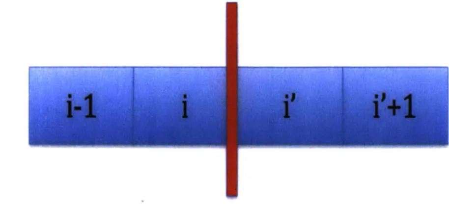
Finally, the PE/Sediment boundary is more complex

- 4

I

₁

'1

-

lm

I

eipil

masmmm6

-

umsmmlsseaise

ns

a

~mm4

Figure 7: Diagram of the grid spatial discretization at the PE/sediment boundary. Using the notations of the diagram above, the boundary condition at x = 1 is:

Ci+1/2,j = Ci-1/2,j X KPESED

2 (Cij - C_+1/2,j)

'E

= 2 DSED (C - j

All the previous relations allow us to build the coefficient matrices to describe our model.

4.2.2

Coefficient Matrices

In the Polyethylene

In the PE, the governing equation is simple and can be translated with the fol-lowing matrices (at a given z coordinate

j):

A x C'+1 = B x C+ E

C+1 = A\(B x C+ E)

With A and B constant Nz x Nx size matrices, E a constant Nx x 1 matrix and Cj also a Nx x 1 matrix but evolving with time:

dx+ _dxa -a 0 .. 0 A 0 - 0 -a 0 ... 0 -a dx+2a dx b b 0 ... ₀ dt b dx -2b_dt B= 0 0 b 0 ... 0 b x -2b dt C1, 0 C = C2,j and E 0 CNx,J 2DPEKPESEDCsed,x=l

(The constant matrix E results from the boundary condition at x 1 but needs

to be updated at every time step as the concentration at the limit of the sediment varies). C +1 is calculated sequentially at each time step until the simulation time

is reached. This allows us to obtain the concentration over the thickness of the PE

after At and at a given height

j,

although CPE is constant in the vertical direction (no processes in z are considered).

In the sediment

The reasoning is identical in the sediment as in the PE. However, since advection is a vertical process, there is a dependence in z and there are more matrices to build. We can calculate C +' with the following relation:

Al x C+1 + A2 x Ct_1 = B1 x C+ B2 x C +F

With Al and BI constant Nz x NX size matrices, A2 and B2 constant Nz x NX size matrices (applied to Cj_1), F a constant NX x 1 matrix and C also a NX x 1 matrix but evolving with time and dependent of Cj_1:

dadz +3adz+wdxO dt -adz -adz dadz+2adz+wdxO 0 0 bdz dxdz _dt -2bdz-wdx(1-0) 0 0 0 ... 0 . '. 0 S - d -a d z o -adz dxdz _dt +2adz+wdxO 0 0 0 '. 0 . bdz bdz dxdz -2bdz-wdx(1-) _ A2= wdX B2= C1,

j

C =C2,j -wdXO 0 0 (1-6) 0 0 0 ... 0 0 ... 0 -wdXO 0 and F = . 0 . 0 wdX(1 - 9) 2 DSED dz Csed,x=l 0 [ CNXJ I 0

J

The matrix F is added to consider the left boundary condition for the sediment. This matrix is also updated at every time step to integrate the changes in the bound-ary concentration.

A1=

d -dz -3bdz-wdx(1-0) bdz

4.2.3

Precision and Stability of the Model

Using the Crank Nicholson approach to model the time-changing concentrations gives not much more numerical expense than the fully implicit approach but is also more accurate. Overall, with this model, we can consider that we have convergence of results if:

At D A 1

Ax2

At is the incremental time step, D the diffusion coefficient and Ax an incremental length. This will always be verified prior to the calculations on Matlab.

Chapter 5

Numerical Simulation Results and

Analysis

5.1

Observing concentration over time

5.1.1

Presentation and Purpose

This section covers the basic result of obtaining the concentration profiles in the polyethylene and the sediment over time with a fixed sediment porewater velocity. The parameters for the profiles in this section are chosen in accordance with the paper by Fernandez et al. [81 which describes a model with only diffusion. Therefore, the chemical we consider is d10-pyrene; the diffusion coefficients for this PRC are

DPE = 3 x 10 10cm2/s and Dsed = 3 x 10-9cm2_{/s; the partitioning coefficient} KPESED is equal to 5; finally, we fix w = 5cm/day to reflect a typical value for infiltration in the environment. The geometry parameters are as follows: height of 10cm, thickness of 100pm and sediment length of 10cm (diffusion transport process is slow enough to consider this length is infinitely long compared to the diffusion length scale in the sediment).

The goal of this initial simulation is to understand the general behavior of the system over time, how concentration evolves and the time scales for PRC depletion in the PE. However, all of these highly depend on the chosen chemical so the results

cannot be considered universally true.

5.1.2

Results and Analysis

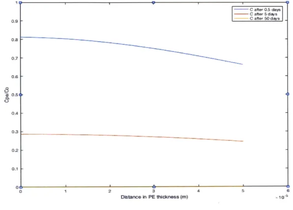
The first numerical model plots the concentration profile of the PRC over the PE's thickness at the height z = h (top of the PE strip):

0.9 0.7 0.6 8 0.6 OA 03 0.2 F 0.1 0 2 3 Distwice in PE ftckness (m) 4 5 X10.6

Figure 8: Concentration profile of PRC over the PE's thickness at various times.

As expected, we can see that the concentration gradually decreases in the PE as the PRC leaves the PE and goes in the sediment. The concentration is highest at

x=0, which is also expected as the boundary x=0 represents the middle of the PE,

therefore the region of maximum concentration at any given time. Also, as the yellow curve shows, all of the d10-pyrene has left the PE by 50 days. This time is highly dependent on the chemical and will be studied in greater detail in the third section of this chapter. The following profiles show the concentration over the sediment length at the same height and at the same specified times: 0.5 days, 5 days and 50 days:

altrO days - C alter 50 das -_ ~~ -4 .L 1& 04 I I

0.121 0.1 01J O 0.064 004 002 I 0 0.1 02 0.3 OA 06S 0l Dstance in sediment in X ("n$ 0.7 0A 0.9 1 S10.

Figure 9: Concentration profile of PRC over the sediment length at various times.

Similarly, the profile shows the PRC infiltrates the sediment at the boundary with the PE and gradually diffuses through the sediment length. The length scale L to define a zone infinitely far from the PE can be very small, as in this case for instance, where any sediment portion further than 1mm away from the PE boundary has a negligible PRC concentration. This is due to the high Kd of d10-pyrene which induces a very small diffusion coefficient in the sediment. L can be adjusted accordingly, and in this case the domain was reduced in x from 10 cm to 1 mm.

Finally, we can plot the concentration profiles along the vertical dimension of the PE. C atar 0.5 day ___Cater5d~ts ----Cater 50 days K on -GRP I - -

--0.7 4 I I 013 05 OA 02 02 0.1 001 0.02 013 044 0135 006 Height fmxn z = 0 in m 0.07 0.08 0139 0.1

Figure 10: Concentration profile of PRC over the PE height at various times.

The graph on Figure 10 is plotted at the PE/sediment boundary in x. The bottom of the PE is in direct contact with sediment containing no PRC at any given time; therefore it is normal to find CPE = 0 for z = 0. Moreover, it is normal to find that

the concentration gradually increases with z because the bottom of the sediment is constantly flushed by "fresh" water containing no PRC. Therefore, the concentra-tion in the sediment is lower for "small" values z, which induces a more important concentration gradient and diffusive flux from the PE to the sediment.

Note: While all the previous concentration profiles seem to be consistent with reality in terms of overall shape and evolution, experimental validation is still required to see if the entire profile is reasonable. Chapter 6 details an experiment to validate the numerical model.

a

Cafte5 dqn

|C aftr 0 days

-5.2

Observing concentration at different infiltration

rates

5.2.1

Presentation and Purpose

The core of this paper is detailing how passive samplers can reflect infiltration velocity in the sediment. The main principle behind this measurement method is that the concentration in the passive sampler depends on this velocity and that experimental data can be fitted with a set of curves of modeled concentrations at different velocities. Thus, using a least squares optimization method for example, we would be able to deduce the porewater velocity from this set of curves for each compound.

Moreover, to obtain sufficient precision on the velocity deduction, the impact of velocity on the profiles needs to be strong enough so that differences can be easily detectable. For instance, if the concentration in the PE with an infiltration speed of 1 cm/day is only 1% higher than with an infiltration speed of 10 cm/day, the differences are too small to deduce from PE extraction which of these two infiltration velocities is more likely in the environment. Therefore, we will also be looking at the differences in amplitude when plotting the concentration profiles at various velocities.

In this section, we plot a set of concentration profiles at different values of w for the same chemical as in the previous section, d10-pyrene. The values of DPE, DSED

and KPESED remain the same, the amount of time the PE is left in the environment is fixed at two days for each simulation, and the velocities are 1cm/day, 10cm/day and 100cm/day.

5.2.2

Results and Analysis

First, the concentration profiles over the PE's thickness after two days are represented in Figure 11. Each curve models the concentration profiles at a given velocity and is plotted at the height z = h.

Is I I I I I I I I 0. -C A --- w = 10 cr da 0 a b 1 1.5 2 M 3 3.5 4 4h 5 Distance iPE im ,106

Figure 11: Concentration profile of PRC over the PE thickness for various sediment porewater velocities after two days.

The first observation we can make is that the average concentration over the PE thickness decreases when the velocity increases. Indeed, the greater the porewater velocity is, the more the sediment is flushed with "fresh" water from z < 0 and there-fore the lower is the concentration in the sediment. This increases the concentration gradient at the PE/sediment boundary and the PRC diffuses from the PE faster.

In terms of amplitude variations, the graph shows that if we observe concentrations at z = h in the PE, there is about a 10% variation on average between velocities of

1 and 10 cm/day, whilst there is a factor of about three between the concentration profile at 100 cm/day and the lower velocity profiles. Therefore, for d1O pyrene, it seems that measurements at z = h can be used to infer velocities greater than 10 cm/day with sufficient precision, but for lower infiltration, the precision is much lower. Can we obtain greater profile variations for low velocities at different PE heights? The following graph plots the concentration profiles over the PE height at

the PE/sediment boundary (x days) as the previous graph:

0.5 OAS I OA 035

8

₀₂₅ 02 0.15 0.1 0jo5

= 1) and for the same velocities and duration (two

0 0.01 0.02 0.03 004 005 06 Distance in PE ower height (m)

Figure 12:

0.07 0.08 Ov.0 0.1

Concentration profile of PRC over height at the PE/sediment interface after two days for various sediment porewater velocities.

We can make three conclusions for d10-pyrene from this plot:

- As w increases, the concentration over the boundary decreases overall. This can be explained for the same reason as the decrease in concentration over the thickness

(cf. Figure 11).

- With the velocity of 1 cm/day, the concentration doesn't evolve in z beyond 2 cm from the bottom. This is because after 2 days, the "fresh" water has only traveled 2 cm so all the PE beyond that behaves as if w = 0. We can conclude that with no infiltration and after two days, the d10 pyrene concentration should be uniformly about 48 % of the initial concentration over the PE/sediment boundary.

- Different heights of the PE need to be sampled to have the best possible precision when deducing the velocity. For instance, for d10-pyrene, the extraction should be

II I I I I I/ 7 7 / / /

K

w = I crt~daj w = 10 cn~daV w =100 crdaV -

7.-at z = h if the infiltr7.-ation is believed to be between 10 and 100 cm/day, whereas the extraction should be at around one tenth of the height for lower velocities. Therefore, the model shows that in theory, PE passive samplers can be used to deduce velocities in the range of what is observed in the environment with sufficient precision.

Figure 13 showcases another method that could be used to velocity.

measure infiltration

0 0.01 0.02 0.3 0.04 005 0.06

Heigt in PE in m

0.07 0.08 009

Figure 13: Concentration profile of PRC over height at the PE/sediment interface after 1 day for various sediment porewater velocities.

Here, like on Figure 12, the concentration in the PE is plotted over height at the PE/sediment for various velocities but only after one day. The chosen porewater velocities are also in the same order of magnitude (1 to 10 cm/day) to better illustrate this method.

As "freshwater" from beneath the PE moves at the velocity w (from left to right on Figure 13), the "transient front", i.e. the decrease in concentration at the boundary induced by this fresh flux, also moves at the velocity w. It is clearly visible that

O. OS I. OA f

a

a 0o3 I I I I - I I, I I I I I I I - I I I I I I I I I I I I I I . . I 0.2 0.1 0 0.1 w 2 crWdaV w 5 crWday vw- 8 crWdaV

after one day, at the velocities of 2 cm/day, 5 cm/day and 8 cm/day, the front has traveled respectively 2 cm, 5 cm and 8 cm up the PE. This distance Zfront can easily be measured during the PE analysis after extraction by cutting the strip into 1 cm strips for instance and detecting where the concentrations are changing in z (freshwater has reached the portion) and where they stay relatively constant (freshwater hasn't reached the portion yet). We can then deduce w by simply writing:

Zfront

At

Note that for this method to work, the front must have traveled less than the height of the PE but also sufficiently to be detectable (at least a tenth of the height for example). This limits the range of infiltration velocities that can be measured using this method but if w is known within one order of magnitude and the height of the PE as well as At are calibrated accordingly, a precise estimate can be provided.

Whilst we can conclude on the passive sampler's theoretical effectiveness in deduc-ing velocity for d1O pyrene, this analysis could change for different chemicals. The ability of passive samplers to deduce porewater velocity needs to be defined every time a new chemical is used.

Chapter 6

Ex situ Validation of Numerical

Model

The numerical results displayed in the previous chapter can only be used as a basis to predict sediment porewater velocity in the environment if these results are validated by experimental data. Therefore, the aim of the following experiments is to recreate in the laboratory a condition where a PE passive sampler in sediment is subject to a known infiltration velocity, and check that the evolution of concentration in the polyethylene follows the numerical evolution.

6.1

Description of the Experiments

6.1.1

Main Setup

First, in order to reproduce conditions close to what is observed in the laboratory, a few key questions need to be answered:

- Which performance reference compound should be impregnated in the PE ini-tially?

- What sediment should be used?

- How can a velocity of the scale of 1-10 cm/day be generated and maintained in the sediment?