Path Deformation Roadmaps

HAL Id: hal-01987454

https://hal.laas.fr/hal-01987454

Submitted on 21 Jan 2019

HAL is a multi-disciplinary open access

archive for the deposit and dissemination of

sci-entific research documents, whether they are

pub-lished or not. The documents may come from

teaching and research institutions in France or

abroad, or from public or private research centers.

L’archive ouverte pluridisciplinaire HAL, est

destinée au dépôt et à la diffusion de documents

scientifiques de niveau recherche, publiés ou non,

émanant des établissements d’enseignement et de

recherche français ou étrangers, des laboratoires

publics ou privés.

Path Deformation Roadmaps

Léonard Jaillet, Thierry Simeon

To cite this version:

Léonard Jaillet, Thierry Simeon. Path Deformation Roadmaps. Algorithmic Foundation of Robotics

VII, 47, Springer Berlin Heidelberg, pp.19-34, 2008, Springer Tracts in Advanced Robotics.

�hal-01987454�

L´eonard Jaillet and Thierry Sim´eon

LAAS-CNRS 7 avenue du Colonel Roche 31077 Toulouse Cedex 4 France ljaillet@laas.fr - nic@laas.fr

This paper describes a new approach to sampling-based motion planning with PRM methods. Our aim is to compute good quality roadmaps that encode the multiply connectedness of the Cspace inside low redundancy graphs, yet representative of the different varieties of free paths. The proposed approach relies on a notion of path deformability indicating whether or not a given path can be continuously deformed to another existing one. By considering a simpler form of deformation than the one allowed between homotopic paths, we propose a method that extends the Visibility-PRM technique [12] to con-struct compact roadmaps that encode a richer and more suitable information than representative paths of the homotopy classes. The Path Deformation Roadmaps also contain additional useful cycles between paths in the same homotopy class that can be hardly deformed into each other. First experi-ments presented in the paper show that our technique enables small roadmaps to reliably and efficiently capture the multiply-connectedness of the space in various problems.

1 Introduction

Robot motion planning has led to active research over the past decades [5] and sampling-based planning techniques have now emerged as a general and effective framework for solving challenging problems that remained out of reach of the previously existing complete algorithms. They allow today to handle the complexity of many practical problems arising in such diverse fields as robotics, graphics animation, virtual prototyping and computational biology. In particular, the Probabilistic RoadMap planner (PRM) introduced in [4, 8] and further developed in many other works (see [2, 6] for a survey) have been conceived to solve multiple-query problems.

While most of the PRM variants focus on the fast computation of roadmaps approximating the connectivity of the free configuration space, only few works [9, 7] address the problem of computing good quality roadmaps that encode the multiply connectedness of the space inside small graphs containing only

useful cycles, ie. cycles representative of the varieties of free-paths. Intro-ducting such cycles is important for getting higher quality solutions when postprocessing queries, thus avoiding the computation of unnecessarily long paths, difficult to shorten by the smoothing techniques (e.g. [10, 13]).

Intuitively, the probability that a roadmap captures well the different paths varieties of Cf ree increases with its degree of redundancy. However, a direct

approach attempting connections between all pair of nodes is far too costly and several heuristic-based connection strategies have been proposed to limit the number of redundant connections. A first way (e.g. [4]) is to limit the con-nection attempts of new samples to the k nearest nodes of the roadmap (or of each connected component). Another variant is to only consider nodes within a ball of radius r centered at the new sampled configuration (e.g. [1]). A more recent technique proposed in [7] only creates cycles between already connected nodes if they are k times more distant in the roadmap than in the configura-tion space. In all cases, the chances to capture the different path varieties of Cf ree notably varies depending on the choice of the k or r parameter.

More-over it is difficult to choose with these heuristic sampling strategies the good parameter values for a given environment. This may result in a significant loss of performance regarding the roadmap construction process.

In this paper we present an alternative method to build compact roadmaps, yet representative of the different varieties of free paths. The method only gen-erates a limited number of useful cycles in the roadmap. Moreover it stops automatically when most of the relevant alternative paths have been found. Our approach relies on a notion of path deformability indicating whether or not a given path can be continuously deformed to another existing one. In comparison with the standard notion of homotopy which is not directly suitable for our purpose because it relies on too complicated deformations (Sect. 2), we consider more simple and easily computable deformations be-tween paths (Sect. 3) that result in compact roadmaps capturing a richer set of paths than homotopy (Sect. 4). We describe in Section 5 a two-stage algo-rithm for constructing such (easy) path deformable roadmaps. The first stage uses Visibility-PRM [12] to construct a small tree covering the space and cap-turing its connected components as well as possible. The second stage aims to enrich the roadmap with new nodes involved in the creation of useful cycles. The key ingredient of this step is an efficient path visibility test used for the filtering of useless cycles that can be easily deformed to the existing roadmap. Following the philosophy of Visibility-PRM, the second stage integrates a stop condition based on the difficulty to find new useful cycles. Finally, our first experiments (Sect. 6) show that the technique enables small roadmaps to re-liably capture the multiply-connectedness of configuration spaces in various problems involving free-flying or articulated robots.

2 Homotopy versus Useful Roadmap’s Paths

We first informally discuss the relation between homotopy and the represen-tative path varieties that it would be desirable to store in the roadmap. The

capture of the homotopy classes of Cf ree corresponds to a stronger property

than connectivity. Two paths are called homotopic (with endpoints fixed) if one can be ”continuously deformed” into the other (see section 3.1). Ho-motopy defines an equivalence relation on the set of all paths of Cf ree. A

roadmap capturing the homotopic classes means that every valid path (even cyclic paths) can be continuously deformed to a path of the roadmap. PRM methods usually do not ensure this property. Only the work of Schmitzberger [9] considers formally the problem and sketches a method for encoding the set of homotopic classes inside a probabilistic roadmap. However, the approach is only applied on two-dimensional problems and its extension is limited by the difficulty to characterize homotopic deformations in higher dimensions.

Fig. 1. A roadmap capturing only the paths of different homotopy would have a unique representation for the two kind of paths presented above.

Moreover, as it was noted in [7] capturing the homotopy classes in higher dimensions might not be sufficient to encode the set of representative paths since homotopic paths (ie. paths in the same homotopy class) may be too hard to deform into each other. This problem is illustrated on the example of the figure 1. Here Cf ree contains only one homotopy class. Therefore, an

homotopy-based roadmap would have a tree structure. Nevertheless, even if the ”topological nature” of the two represented paths is the same, their dif-ference is such that it seems preferable to store both paths in the roadmap.

Generalizing this idea, we say that a roadmap is a good representation of the varieties of free paths if any path can be ”easily” deformed into a path of the roadmap. This notion of simple path deformation is formalized below.

3 Complexity of a Path Deformation

In this section, after reminding the definition of a homotopic deformation, we propose a way to characterize classes of path deformations according to their complexity.

3.1 Homotopy

The homotopy between two paths is a standard notion from Topology (see a complete definition in [3]). Two paths τ and τ0 in a topological space X are homotopic (with end points fixed) if there exists a continuous map h : [0, 1] × [0, 1] → X with h(s, 0) = τ (s) and h(s, 1) = τ0(s) for all s ∈ [0, 1] and h(0, t) = h(0, 0) and h(1, t) = h(1, 0) for all t ∈ [0, 1].

Homotopy is a way to define any continuous deformation from one path to another. Next, we introduce a less general class of deformations, called K-order deformations characterizing particular subsets of homotopic deformations and that is used in section 4 for computing path deformation roadmaps.

3.2 K-order Deformation

Definition 1. A K-order deformation is a particular homotopic deformation such that each curve transforming a point of τ into a point of τ0 is an angle line of K segments. τ τ! τ τ! τ τ! a b c

Fig. 2. (a) general homotopic deformation. (b) first order deformation: the defor-mation surface is a ruled surface. (c) Second order defordefor-mation: the defordefor-mation surface is obtained by concatenating two ruled surfaces.

Therefore, a first-order deformation surface describes a ruled surface and a K-order deformation is obtained by concatenation of K ruled surfaces. This is illustrated by figure 2 that shows different types of path deformations: (a) is a general homotopic deformation whereas (b) and (c) show respectively 1st-order and a 2nd-order deformations.

Let Di denote the set of i-order deformations. We clearly have Di ⊂

Dj _{for all i < j. Thus, the value K of the smallest K-order deformation}

ex-isting between two paths is a good evaluation of the difficulty to deform one path into the other.

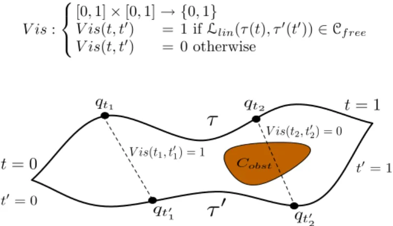
3.3 Visibility Diagram of Paths

It is important to note that a first-order deformation between two paths exists if and only if it is possible to simultaneously go through the two paths while

maintaining a visibility constraint between the points of each path (see figure 3). This formulation provides a computational way to test the existence of a first-order deformation, also called visibility deformation between two paths. Let Llin be the straight line segment between two configurations of C. The

parametric visibility function V is of two paths (τ, τ0) is defined as follows:

V is :  



[0, 1] × [0, 1] → {0, 1}

V is(t, t0) = 1 ifLlin(τ (t), τ0(t0)) ∈Cf ree

V is(t, t0) = 0 otherwise

t

= 0

t

_{= 1}

τ

τ

q

Fig. 3. The parametric visibility function of two path evaluates the visibility between the points of each path.

Then, the visibility diagram of paths (τ, τ0_{) is defined as the two}

dimen-sional diagram of the function V is, as illustrated by the figure 4 showing sev-eral examples of computed visibility diagrams with the corresponding paths. Thanks to the visibility diagram, the visibility (i.e. first-order) deformation between two paths can now be expressed as follows: two paths (τ , τ0) (with the same endpoints) are deformable by visibility one into the other if and only if there is a path in their visibility diagram linking the points of parameters (0, 0) and (1, 1). Therefore it is possible to test the visibility deformation between two paths by computing their visibility diagram and then searching for a path in the diagram linking the points (0, 0) and (1, 1). In figure 4, such a deformation is only possible for the last example (d).

4 K-order Deformation Roadmap

In the previous section we have defined a way to characterize the complexity for two paths to be deformed one into the other. This formalism is now used to define for a given roadmap its ability to capture the different varieties of free paths of the configuration space.

Definition 2. A roadmap R is a K-order deformation roadmap if and only if for every path τ of Cf ree it is possible to extract a path τ0 from R (by

connecting the two extremal configurations of the paths) such that τ and τ0 are K-deformable.

init goal Init goal init goal

a

b

c

d

c

Fig. 4. Visibility diagrams for pairs of paths with the same endpoints. White areas represent regions where V is(t, t0) = 1. A visibility deformation is only possible in the last example (d), where a valid path linking the points (0,0) and (1,1) can be found in the visibility diagram.

This definition establishes a strong criterion specifying how the different varieties of free paths are captured inside the roadmap. One can also note that since a K-order deformation is a specific kind of homotopic transfor-mation, any deformation roadmap captures the homotopy classes of Cf ree.

The following subsections present a computational method to construct such roadmaps.

4.1 Visibility Deformation Roadmap

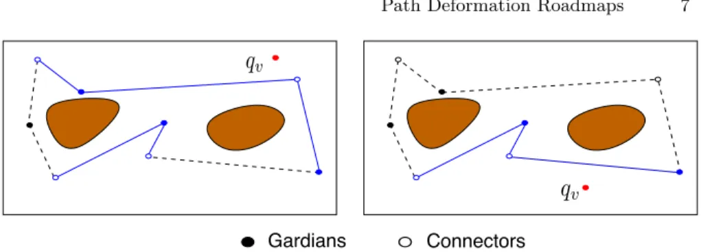
We first define the notion of Roadmap Connected from any Point of View (called RCPV roadmaps) previously introduced in [9]. We then establish that RCPV roadmaps are visibility (i.e. first-order) deformation roadmaps. Visible Subroadmap

Let R be a roadmap with a set N of nodes and a set E of edges. If R cov-ers Cf ree, we can extract a set of nodes Ng (called guardians) maintaining

this coverage. Then, we can define for a free configuration qv, the Visible

Subroadmap Rv= (Nv, Ev), as follows :

• Nvsublist of guardians visible from qv: Nv= {n ∈ Ng/Llin(qv, n) ∈Cf ree}

• Ev, sublist of edges visible from qv: Ev= {e ∈ E/Llin(qv, e) ∈Cf ree}

Note that the notationLlin(qv, e) ∈Cf ree means that {∀q ∈ e, L(qv, q) ∈

Cf ree}. Examples of visible subroadmaps are presented in figure 5.

RCPV Roadmaps

Definition 3. A Roadmap Connected from any Point of View (or RCPV roadmap) is such that for any configuration of Cf ree, the visible subroadmap

q

q

Gardians Connectors

Fig. 5. Two examples of visible subroadmap from a given configuration qv. On the

left, the visible subroadmap is disconnected whereas it is connected on the right.

The following property establishes the link between RCPV roadmaps and visibility deformation roadmaps.

Property: A RCPV roadmap is a particular case of visibility deformation roadmap.

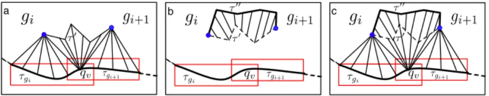
Sketch of proof: Let R be a RCPV roadmap and τ , a path ofCf ree. τ can

be partitioned into 2n − 1 successive paths:

τ = {τg1⊕ τg1∩g2⊕ ... ⊕ τgi⊕ τgi∩gi+1⊕ τgi+1⊕ ...τgn−1⊕ τgn−1∩gn⊕ τgn}

with τgi denoting the portion of path only visible from the giguardian and

τgi∩gi+1 the portion visible simultaneously from gi and gi+1. Since τgi and gi

are by definition visible, it is possible to build a patch of ruled surface between them (figure 6.a). Similarly, there is a patch of ruled surface between τgi+1and

gi+1. Because R is a RCPV roadmap, any configuration qv ∈ τgi∩ τgi+1sees a

path τ0 connecting gi to gi+1. This property allows to build a third patch of

ruled surface between qv and τ0 (figure 6.b). Finally, it is possible to extract

from these three patches a global ruled surface between τgi ∩ τgi+1 and τ

0

(figure 6.c). Thus, there exists a ruled surface (i.e. a visibility deformation surface) between the totality of τ and a path of the roadmap.

g

g

τ

g

g

τ

g

g

τ

Fig. 6. A RCPV roadmap is a visibility deformation roadmap. (a) the visibility of the guardians gives first patches of ruled surfaces. (b) the RCPV roadmap prop-erty guarantees the visibility of a roadmap path connecting two guardians. (c) By construction, a global visibility deformation surface can be built.

RCPV roadmaps are first-order deformation roadmaps. However, these roadmaps involve a high level of redundancy (see results section 6) and yet contain many useless cycles, especially in constrained situations. Therefore, to keep a compact structure we filter a part of the redundancy as explained in the following section. We will show that this filtering leads to a second-order deformation roadmap.

4.2 Second-order Deformation Roadmaps

Let R be a RCPV roadmap, Ng ∈ R be a set of guardian nodes ensuring

the Cf ree coverage. Let consider a pairs of guardians and τ , τ0 two paths of

the roadmap linking theses guardians (i.e. creating a cycle) and visibility de-formable one into the other. Then we have the following property:

Property: From a RCPV roadmap, the deletion of a redundant path τ0 (i.e. visibility deformable into a path τ and connecting the same guardians) leads to a second order deformation roadmap.

Sketch of proof: Let consider the partition of a free path τ , as defined sec-tion 4.1. In that secsec-tion we have shown that with a RCPV roadmap, one can extract a roadmap path τ0 such that τgi∩ τgi+1 is visibility deformable into

τ0 (figure 7.a). Now suppose that the redundant paths τ0 have been deleted as proposed above. Then each deleted path τ0 is visibility deformable into another path τ00 which remains in the roadmap (figure 7 b). Then, by con-catenation of the two ruled surfaces it is possible to build a second order deformation surface between each path of Cf ree and a path of the roadmap

(figure 7 c).

g

g

g

g

g

g

Fig. 7. Deleting redundant paths in a RCPV roadmap leads to a second-order deformation roadmap. (a) Visibility deformation for a RCPV roadmap. (b) A filtered path is itself deformable by visibility into a roadmap path. (c) By construction, there is a second-order deformation surface between a free path and a portion of roadmap.

Based on this notion of deformation roadmap, we describe below a com-putational way for constructing such roadmaps.

5 Algorithm for building Deformation Roadmaps

First, the roadmap is initialized with a tree structure computed with the Visibility-PRM method [12]. This ensures the coverage of the free space with

a limited number of nodes and edges (i.e. no cycles). Then, instead of first building a RCPV roadmap and filtering in a second step the redundant cycles (as defined section 4.2), the redundancy test is directly performed for effi-ciency purpose before each addition of a new cycle to the roadmap.

The pseudo-code of the algorithm used to build a second-order deformation roadmaps is shown in figure 8. At each iteration a free configuration qvis

ran-domly sampled and the connectivity of the visible subroadmap is computed (TestVisibConnection function line 5). The evaluation of its connectivity is performed avoiding as much as possible the whole computation of the sub-roadmap. the redundancy test is only performed when the visible subroadmap is disconnected. for this test, we choose randomly two disconnected compo-nents of the subroadmap and choose among them the nearest nodes n1, n2,

from qv. Then, we test if there is a visibility deformation between the path

τ = n1− qv− n2 and a path of the roadmap (TestVisDefo function line 9).

If such visibility deformation exists, the configuration is useless regarding the construction of a second-order deformation roadmap and is therefore rejected. The algorithm memorizes the number of successive failure since the last useful cycle inserted and uses this information to stop when the insertion of a new cycle becomes too hard, meaning that most of the useful cycles are already captured by the roadmap.

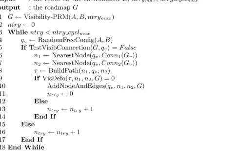
DEFORMATION PRM

input : the robot A, the environment B, ntrymax, ntry cyclmax

output : the roadmap G

1 G ← Visibility-PRM(A, B, ntrymax)

2 ntry ← 0

3 While ntry < ntry cyclmax

4 qv← RandomFreeConfig(A, B) 5 If TestVisibConnection(G, qv) = F alse 6 n1← NearestNode(qv, Conn1(Gv)) 7 n2← NearestNode(qv, Conn2(Gv)) 8 τ ← BuildPath(n1, qv, n2) 9 If VisDefo(τ, n1, n2, G) = 0 10 AddNodeAndEdges(qv, n1, n2, G) 11 ntry← 0 12 Else 13 ntry← ntry+ 1 14 End If 15 Else 16 ntry← ntry+ 1 17 End If 18 End While

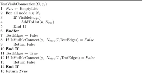
We next detail the algorithms used to establish the subroadmap connec-tivity (TestVisibConnection function) and to test the visibility deformation between pairs (TestRetract function).

5.1 Visible Subroadmap

The method establishing the connectivity of a visible subroadmap from a given configuration qv (TestVisibConnection function in the Def ormation P RM

algorithm) corresponds to the pseudo-code of figure 9. First, the number of nodes visible from qv is computed by testing if the straight line segments

linking qv to each of the roadmap nodes are free. Then, we test in two phases

the connectivity of these nodes from the point of view of qv. First, we evaluate

all the roadmap’s edges as potentially visible. Thus, two nodes are detected disconnected if all the paths of the roadmap connecting them pass through at least one invisible node (IsVisibleConnect function line 8). If this fast test is not sufficient to establish the connectivity of the visible subroadmap, we establish it by computing the visibility of the edges linking the visible nodes (IsVisibleConnect function line 12). We describe in the next section how the visibility of an edge from a given configuration can be tested.

TestVisibConnection(G, qv)

1 Nvis← EmptyList

2 For all node n ∈ Ng

3 If Visible(n, qv)

4 AddToList(n, Nvis)

5 End If 6 Endfor

7 TestEdges ← False

8 If IsVisibleConnect(qv, Nvis, G,TestEdges) = F alse

9 Return False 10 End If

11 TestEdges ← True

12 If IsVisibleConnect(qv, Nvis, G ,TestEdges) = F alse

13 Return False 14 End If

15 Return T rue

Fig. 9. Algorithm testing the visible subroadmap connectivity from a given configu-ration qv.

5.2 Edge Visibility

Testing the visibility of an edge from a configuration qvis equivalent to

check-ing the validity of a configuration space triangular facet, defined by qv and

the two edge’s endpoints (c.f. figure 10). Note that this visibility test possibly requires several facet tests depending on the topological nature ofC:

n

n

q

Fig. 10. Edge visibility: n1−n2 is visible from qv if the facet {qv, n1, n2} is valid.

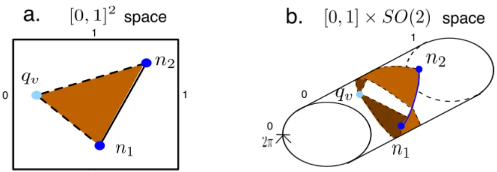
• IfC is isomorphic to [0, 1]n _{(the robot’s degrees of freedom are only}

trans-lations and/or bounded rotations) then the visibility test can be done by testing only a single facet inC (figure 11(a)).

• IfC is isomorphic to [0, 1]n_{× SO(d)}m_{with m > 0 (one or more degrees of}

freedom are cyclic), the visibility test of an edge can lead to test several facets (figure 10(b)). Actually a discontinuity occurs each time the distance between qv and a configuration on the edge is equal to π according to a

given degree of freedom.

[0

,

1]

[0, 1] × SO(2)

q

q

n

n

n

n

a.

space

b.

space

2π

Fig. 11. Testing the visibility of an edge can lead to test one (a) or several (b) facets, depending of the topological nature of the configuration space.

5.3 Elementary Facet Test

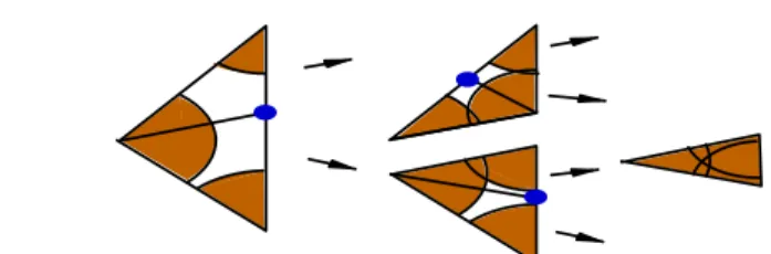
To test the validity of a facet we try to cover it entirely with free balls ofC (figure 12). First, the radius of the balls centered on each vertex of the facet are computed using a conservative method based on the robot kinematics and the distance of its bodies to the obstacles. If the balls are sufficient for covering the facet, then the algorithm returns that the facet is valid. Otherwise it is split into two sub-facets such that their common vertex is as far as possible from the regions already covered by the balls. The radius of the ball centered on this vertex is then computed. This dichotomic process is performed until the entire facet is covered or one vertex is tested as invalid.

Fig. 12. Dichotomic covering of a valid facet withCf ree balls.

5.4 Redundancy Test

A disconnected subroadmap from the point of view of a configuration qv can

be reconnected by linking two of the subcomponents through qv. Before

per-forming such connection attempt, we test if it would not lead to a redundant path which could be filtered. To do so, we build first the path τ = n1−qv−n2

with n1, n2 belonging to two distinct subcomponents. Then we test its

visi-bility deformation into a roadmap path thanks to the VisDefo algorithm (line 9 in figure 8). This algorithm is shown in figure 13. Roadmap paths are itera-tively extracted and tested according to their visibility deformation relaitera-tively to τ . This process starts with the shortest path found and stops when a vis-ible deformation is found (then the configuration is rejected) or when all the possible paths have been tested (then the configuration and the edges n1−qv

and n2−qv are inserted).

VisDefo(τ, n1, n2, G) 1 τ0← BestPath(n1, n2, G) 2 While τ0_{6= ∅} 3 If IsVisDefo(τ, τ0) = 1 4 Return 1 5 End If 6 τ0← BestPath(n1, n2, G) 7 End While 8 Return 0

Fig. 13. Visibility deformation test between a path τ and a roadmap path.

The IsVisDefo function (line 3 of algorithm 13) tests if two paths τ and τ0 can be visibility deformed one into the other. This function is based on the computation of the visibility diagram associated to the two paths with a grid method. The deformation is only possible when there exists a path between the (0, 0) and (1, 1) points in this diagram (c.f. section 3.3). In practice, the whole diagram is not computed and the tests are limited to the elements of the grid visited during the A∗ search of a ”valid path” in the visibility diagram, incrementally developed during the search. This implicit search of the diagram notably limits the number of visibility tests to be performed (figure 14) and highly speeds up the redundancy test.

Fig. 14. Visibility diagram (left) and the portion really explored (right) for a visibility deformation test between two paths.

6 Experimental Results

We implemented the algorithm for contructing (second-order) deformation roadmaps in the Move3D software plateform [11]. The experiments reported below were performed on a 1.2GHz G4 PowerPC running on Mac OS-X. The performance results summarized in Table 2 correspond to average values com-puted over several runs of the algorithm.

The first experiment shown on figure 15 compares the level of redundancy obtained in function of the algorithm used: (a), a minimum tree structure ob-tained with the Visibibility-PRM, (b) a first-order roadmap (build without the filtering process) and (c) a second-order deformation roadmap that captures the different varieties of paths while maintaining a compact structure.

b c

a

Fig. 15. Comparison between three algorithms of roadmap construction. (a) Visibility-PRM. (b), first-order and (c), second-order deformation roadmap.

The next set of experiments (figure 16) presents the deformation roadmaps obtained for a 2-dof robot evolving in more complex environments. The first scene (a) requires 29 elementary cycles to capture the homotopy. Our method is able to build a roadmap capturing these cycles in only 109 seconds . The second scene (b) has a higher geometrical complexity (70 000 facets). The computing time (164 sec.) reported in Table 2 shows that the algorithm can efficiently handle such geometrically complex scenes. One can also note that the resulting 2D roadmaps contain a very limited number of additional nodes compared to homotopy.

a b

Fig. 16. Deformation Roadmaps for 2D environments: (a) a labyrinth with many homotopy classes. (b) an indoor environment with a complex geometry.

The third experiment (figure 17) involves a narrow passage problem for a squared robot with 3-dofs (two translations and one rotation). The robot has four ways to go through the narrow passage, depending on its orientation. Therefore the narrow passage corresponds to four homotopy classes in the configuration space. x y 0 Π 2 y x θ Π 3Π 2 c a b

Fig. 17. Deformation roadmap capturing the four homotopy classes for a rotat-ing square and a narrow passage. (a) (x,y) view of the deformation roadmap, (b) (y,θ) view of the same roadmap showing the four kind of passages found inC, (c) comparison with the dense roadmap obtained with a classic k-nearest PRM.

Table 1. Homotopy classes found by a k-nearest PRM for the problem of figure 17. n classes time (s) k 10 20 100 10 20 100 N 1000 0.1 0.2 1.2 6.4 9.3 33.2 2000 0.1 0.6 1.6 33.2 43.5 110.0 4000 0.8 1.0 2.8 246 336 455 8000 1.4 2.4 3.2 2947 3295 3819

Table 1 presents results obtained with a traditional k-nearest PRM [4] for different couples (N, k) (with N, the number of roadmap nodes). The reported results (averaged over several runs) show that even for the most dense and redundant case (N = 8000, k = 100), the homotopy is not well

captured (n classes = 3.2/4) by the k-nearest PRM. Moreover, the large size of the computed roadmap results in a significant computing time (3819 secs) due to the amount of collision tests required for adding new nodes and edges. Comparatively, our method captures the four homotopy classes in only 37 secs. The high speed-up comes from the very compact size of the path deformation roadmap (only 12 nodes) which largely compensates the additionnal cost for filtering the useless redundant cycles.

The last set of experiments (figure 18) involves 6-dof robots in 3D en-vironments. In the first case (free flying robot), the free space has only one homotopy class. Thus, a roadmap based on homotopy would have a tree struc-ture. The results show that our method is able to build a compact roadmap (in 56 secs) while capturing a richer variety of paths than the homotopy. The second scene concerns a 6-dofs manipulator arm where 6 additional nodes (and 12 edges) are added to the visibility roadmap (total time of 100 secs) to represent the complexity of the space. In both cases, the yet limited number of roadmap’s cycles allows to find shorter paths during the query phase.

Finally, the performance results are summarized in Table 2 which also provides a breakup of the total computing time showing the respective con-tribution between the visibility tree building and the cycle addition stages.

a

Fig. 18. Deformation Roadmaps for complex environments: (a) free flying robot, (b) 6-dof manipulator arm.

Table 2. Computing time of the Deformation Roadmaps. time repartition (%)

dof nodes edges cycles time (s) Vis-PRM TestVisConn VisDefo Other Laby 2 149 177 29 109 19 32 35 14 Indoor 2 66 83 18 164 25 20 49 6 Square 3 12 14 3 37 24 61 11 4 Helico 6 30 39 10 56 5 9 80 6 Arm 6 41 46 6 99 12 70 13 5

7 Conclusion

We have presented a general method to build roadmaps with useful cycles rep-resentative of the different varieties of free paths of the configuration space.

The introduction of these cycles is important for obtaining higher quality solu-tions when postprocessing queries inside the roadmap. Our approach is based on the notion of path deformability indicating whether or not a given path can be easily deformed into another one. Our experiments show that the method enables small roadmaps to reliably capture the multiply-connectedness of pos-sibly complex configuration spaces. Several improvements remain for future work. First, the method has been currently tested for free flying and articu-lated robots with up to 6 dofs. We need to further evaluate its performance for higher dof articulated robots. Also, we would like to further investigate the link between the varieties of free paths stored in the roadmap and the smooth-ing method used to shorten the solution paths when postprocesssmooth-ing queries. Finally, another improvement concerns the extension to robots with kinemat-ically constrained motions requiring the use of non-linear local method.

References

1. R. Bohlin and L.E. Kavraki. Path planning using lazy prm. IEEE Int. Conf. on Robotics and Automation, pages 521–528, 2000.

2. H. Choset, K.M. Lynch, S.Hutchinson, G. Kantor, W. Burgard, L.E.Kavraki, and S. Thrun. Principles of robot motion. MIT Press, 2005.

3. A. Hatcher. Algebraic Topology. Cambridge University Press, 2002. Available at http://www.math.cornell.edu/ hatcher/AT/ATpage.html.

4. L.E. Kavraki, P. Svestka, J.-C. Latombe, and M.H. Overmars. Probabilistic roadmaps for path planning in high-dimensional configuration spaces. IEEE Transactions on Robotics and Automation, 12(4):566–580, 1996.

5. J.-C. Latombe. Robot Motion Planning. Kluwer Academic Publishers, 1991. 6. S.M. LaValle. Planning Algorithms. Cambridge University Press, 2004-2005.

Available at http://msl.cs.uiuc.edu/planning/.

7. D. Nieuwenhuisen and M.H. Overmars. Useful cycles in probabilistic roadmap graphs. IEEE Int. Conf. on Robotics and Automation, pages 446–452, 2004. 8. M.H. Overmars and P. Svestka. A probabilistic learning approach to

mo-tion planning. In K. Goldberg et al (Eds), editor, Algorithmic Foundations of Robotics (WAFR1994), pages 19–37. A.K. Peters, 1995.

9. E. Schmitzberger, J.L. Bouchet, M. Dufaut, W. Didier, and R. Husson. Capture of homotopy classes with probabilistic road map. IEEE/RSJ Int. Conf. on Robots and Systems, 2002.

10. S. Sekhavat, P. Svestka J.-P. Laumond, and M.H. Overmars. Multi-level path planning for nonholonomic robots using semi-holonomic subsystems. Interna-tional Journal of Robotics Research, 17(8):840–857, 1998.

11. T. Sim´eon, J.-P. Laumond, and F. Lamiraux. Move3d: a generic platform for path planning. IEEE Int. Symp. on Assembly and Task Planning, 2001. 12. T. Sim´eon, J.-P. Laumond, and C. Nissoux. Visibility-based probabilistic

roadmaps for motion planning. Advanced Robotics Journal, 14(6):477–494, 2000. 13. G. S´anchez and J.-C. Latombe. On delaying collision checking in prm planning - application to multi-robot coordination. International Journal of Robotics Research, 21(1):5–26, 2002.