Aggregation Semantics for Link Validity: Technical Report
Texte intégral
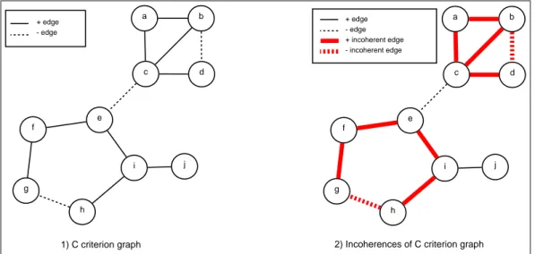
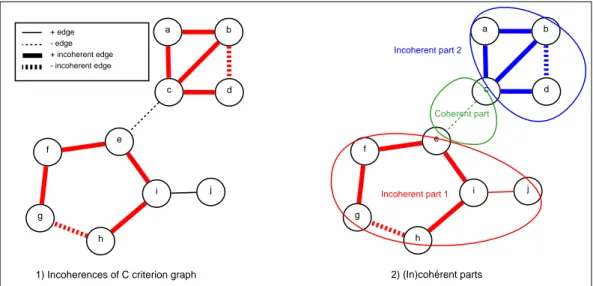
Figure
Documents relatifs
In multi-criteria optimization, one tries to approximate a set of solutions (the Pareto curve) with another set of solutions (the ε-approximate Pareto curve) and the more the
A fragmentation process is a Markov process which describes how an object with given total mass evolves as it breaks into several fragments randomly as time passes. Notice there may
The LIG search system [1] uses a user-controlled combina- tion of six criteria: keywords, phonetic string (new in 2009), similarity to example images, semantic categories, similarity
We will see, by counterexamples in L 2 , that in general, the martingale-coboundary decomposition in L 1 , the pro- jective criterion, and the Maxwell–Woodroofe condition do not
Delano¨e [4] proved that the second boundary value problem for the Monge-Amp`ere equation has a unique smooth solution, provided that both domains are uniformly convex.. This result
We then provide the results of an extensive experimental study of the distributional properties of relevant measures on graphs generated by several stochastic models, including
We developed a method called noc-order (pronounced as knock-order, based on NOde Centrality Ordering) to rank nodes in an RDF data set by treating the information in the data set as
In this paper, for every possible leave graph (excess graph), we find a corresponding maximum packing (minimum covering) of the complete graph with stars with up to five
