Analysis of shock propagation in the magnetosheath

Analysis of Shock Propagation in the

Magnetosheath

by

Aletta M. J. Wallace

Submitted to the Department of Earth, Atmospheric,

and Planetary Sciences

in partial fulfillment of the requirements for the degree of

Bachelor of Science in Planetary Science and Astronomy

at the

MASSACHUSETTS INSTITUTE OF TECHNOLOGY

ARCHIVES

June 2003

Aletta M. J. Wallace, MMIII. All rights reserved.

The author hereby grants to MIT permission to reproduce and

distribute publicly paper and electronic copies of this thesis document

in whole or in part.

Author ...

Signature redacted...

&'Department of Earth, Atmospheric,

/1 h V /)

Signature

redacted

I

and Planetary Sciences

May 15, 2003

Certified by....

V/

Alan J. Lazarus

Senior

esearch Scientist, Department of Physics

Thesis

Accepted

by.Signature

redacted

Brian Evans

Professor, Department of Earth, Atmospheric,

The author _{hereby grants to MIT permission to}

reproduce and to distribute pubicly paper and electronic copias of this thesis document in

and Planetary Sciences

MASSAHSETT I FUTmE

OFTECHNOL00GY

OCT

2 4 2017

Analysis of Shock Propagation

in the Magnetosheath

Aletta M. J. Wallace

June 2003

Analysis of Shock Propagation in the Magnetosheath

by

Aletta M. J. Wallace

Submitted to the Department of Earth, Atmospheric, and Planetary Sciences

on May 15, 2003, in partial fulfillment of the requirements for the degree of

Bachelor of Science in Planetary Science and Astronomy

Abstract

Four interplanetary shock waves and disturbances are analyzed. Data recorded by multiple spacecraft are compared in order to determine how the speed of these events is modified when they cross Earth's bow shock into the magnetosheath. To accom-plish this, it was necessary to find shocks that were seen by spacecraft both in the solar wind and inside the magnetosheath. Using a velocity coplanarity and a Rankine-Hugoniot methods of shock normal analysis, the speeds of these events in the solar wind were calculated. The time of their arrival at a spacecraft in the magnetosheath was determined. The predicted arrival time, assuming a constant shock speed from the spacecraft in the solar wind to the spacecraft in the magnetosheath is then com-pared to the actual arrival time. The resulting data support the conclusion that there is no change in the speed of the shock as it propagates through the magnetosheath. Thesis Supervisor: Alan J. Lazarus

Acknowledgments

The study of shocks in the magnetosheath is supported by grant ATM-9815089 from the National Science Foundation. General analysis of data from the SWE Faraday cups on the Wind spacecraft is supported by NASA grant NA6-10915. This research was carried out using the facilities of the Space Plasma Group at MIT's Center for Space Research.

I would like to thank Dr. Alan Lazarus and Dr. Justin Kasper for their constant help and guidance. Justin has been invaluable in this process, teaching me anything and everything I need to know about the solar wind and coming up with all the kludges I needed to complete my data analysis. I would also like to thank Dr. John Richardson for setting me on this project in the first place and being a valuable resource along the way; and Anne MacAskill for all her encouragement.

Finally, I never could have done this without the support of my parents or the infinite patience of Richard Tibbetts, which I will be repaying when he is finishing his thesis.

Introduction

1.1 Solar Wind . . . . 1.2 Interplanetary Shock Waves . . . . 1.3 Magnetosheath . . . . Previous Work . . . . Instrumentation . . . . 3.1 Advanced Composition Explorer (ACE) . . . 3.2 Wind Spacecraft . . . . 3.3 Interplanetary Monitoring Platform 8 (IMP-8) Data Analysis . . . . 4.1 Finding Shock Pairs . . . ... . 4.2 Shock Analysis . . . . 4.3 Determining Delay . . . . Results: Shocks Seen in Magnetosheath . . . . 5.1 January 11, 2000 . . . . 5.2 July 11, 2000 . . . . Results: Shocks Passing into Magnetosheath . . . . . 6.1 October 28, 1999 . . . . 6.2 January 22, 2000 . . . . 7 Conclusion .

Contents

1

Introduction

Humans have been aware of effects of the solar wind, namely the aurorae, since pre-historic times (Kivelson and Russell, 1995, p.1). Only in the latter half of the twentieth century did we begin to truly understand what the solar wind is and how it works. The past decade has led to an increased interest in shocks in the solar wind due to their adverse interactions with satellites orbiting Earth. Here I have set out to analyze how these shocks behave when they are close to Earth, namely, in the magnetosheath.

1.1

Solar Wind

The solar wind is a diffuse flow of ionized plasma which is constantly being ejected from the Sun. Its existence is due to the fact that the Sun's surface, the corona, is so hot that hydrogen and helium gases can become energetic enough to escape the Sun's gravity. This outward streaming coronal gas was identified by Eugene Parker in

1959 (Parker, 1963). Due to the rotational motion of the Sun, the solar wind flowing

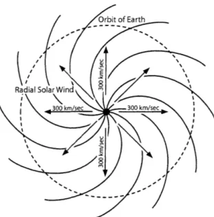
radially out from a source on the Sun traces an Archimedean spiral (Figure 1) as it travels radially. As the solar wind flows outward, it drags with it the solar magnetic field, creating an interplanetary magnetic field (IMF) which propagates out to the edge of the heliosphere, where it encounters the interstellar medium, thought to be at about 120 AU.

1.2 Interplanetary Shock Waves

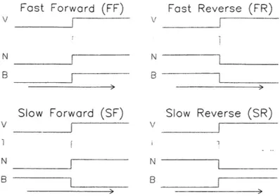
The solar wind is supersonic and travels at an average speed of 400 km/sec, with an average density of 4 particles/cc at 1 AU. Interplanetary shock waves pass through the solar wind causing sudden changes in its parameters. Shocks form when plasma tries to flow faster than the local wave speed. There are four types of shocks, distinguished

by the changes in density, temperature, speed, and magnetic field, as illustrated in

Figure 2 (Kasper, 2002). All the shocks that were looked at in this study are the most common type, fast forward (FF) shocks, where the velocity, temperature, density, and

Orbit of Earth

Radial Solar Wind

300 km/sec 300 km/sec

Figure 1: The solar wind traces out an Archimedean spiral, the so-called "garden hose" effect, caused by the Sun's rotation.

magnetic field all increase as the shock passes the spacecraft.

Coronal mass ejections (CMEs) or corotating interaction regions (CIRs) can cause these shock waves. A CME occurs when the configuration of magnetic fields in the corona becomes unstable. As the CME expands outwards into the corona it runs into coronal material and generates a shock front. CIRs create shock waves when a region of fast solar wind follows a region of slow solar wind in the corona, and due to the Sun's rotation, the fast region "catches up" to the slow as it travels outward (Rasinkangas, 1999). Shocks caused by CIRs are rarely seen at 1 AU, and most at Earth's orbit are caused by CMEs. The frequency of shocks varies over the solar cycle, with maxima every eleven years.

1.3

Magnetosheath

As the solar wind streams out through the solar system it encounters planets with magnetic fields, particularly the Earth. Earth's magnetic field deflects the highly conducting solar wind around it forming a boundary called the magnetopause. The region inside the magnetopause where Earth's magnetic field dominates is called the

Fast Forward (FF) Fast Reverse (FR)

V

N N

B B

Slow Forward (SF) Slow Reverse (SR)

V

N N

B B

Figure 2: The velocity V, temperature T, density N, and magnetic field B profile s of the four types of shocks seen in the interplanetary medium. The colored curves indicate what a spacecraft would observe as each of the shock types traveled past it. In each case time increases to the right as indicated by the arrows.

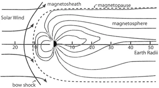
magnetosphere. Since the solar wind is traveling supersonically, an upstream shock, the bow shock, exists where the wind's component of velocity perpendicular to the shock slows to subsonic speed before reaching the magnetopause (Kivelson and Rus-sell, 1995, p.135). In between the bow shock and the magnetopause lies the magne-tosheath. The velocity of the wind is deflected as it crosses the bow shock into the magnetosheath. The layout of this system can be seen in Figure 3.

Interplanetary shock waves are deflected along with the solar wind in the mag-netosheath. It is unclear, though, how their parameters, particularly velocity, are modified when they cross the bow shock. Here this phenomenon is examined by look-ing at the same shock when it is in the wind, and then in the sheath, uslook-ing data from the ACE, Wind, and IMP-8 spacecraft; shock normals are calculated using the ve-locity coplanarity and Rankine-Hugoniot analysis methods. The veve-locity coplanarity method assumes that the difference in the velocity of the wind before and after the shock define the shock normal, the direction in which the shock is propagating. The Rankine-Hugoniot method works by assuming conservation of energy and momentum.

magnetosheath _{_ magnetopause} Solar Wind magnetosphere 20 0 0 40 50 Earth Radii bow shock

Figure 3: Summary of the near-Earth space environment. (Adapted from http://www.sciencenet.org.uk/database/Physics/Sun/. Used with permission.)

2

Previous Work

Villante et al. (2003) describe an experiment where they attempted to determine the propagation speed of shocks in the magnetosheath. They used a Rankine-Hugoniot analysis of shocks to find the shock speeds in the solar wind. Assuming a constant velocity, they then predicted when the shock would reach the bow shock. By com-paring this prediction to the time when the shock reached Earth according to the observation of a geomagnetic disturbance time (Dst), they calculated an estimate of the time it took the shock to travel from the bow shock to Earth, and thus of how fast it traveled. Their results show that shocks traveled at 1/3 to 1/4 of their speed in the solar wind when in the magnetosheath.

3

Instrumentation

3.1

Advanced Composition Explorer (ACE)

Measurements from the Advanced Composition Explorer (ACE) satellite are used here for observing shocks in the solar wind. ACE is in a halo orbit about L1, the first

Lagrangian point, where the gravitational pull of the Sun on a satellite is reduced

by the pull of the Earth to the point that the satellite will orbit the Sun with the

same period as Earth. This point lies 1/ 1 5 0th of the way from Earth to the Sun.

Generally, the spin axis of the ACE spacecraft is along the Earth-Sun line and most of the scientific instruments are located on the sunward side.

The plasma instrument on ACE is a curved-plate electrostatic analyzer (McComas et al., 1998). It is part of the Solar Wind Electron Proton Alpha Monitor (SWEPAM) which is designed to measure the elemental and isotopic composition of the solar wind.

A magnetometer system mounted on booms on opposite side of the ACE spacecraft

measures the magnitude and direction of the local IMF (Smith, 2001).

3.2 Wind Spacecraft

The Wind spacecraft saw shocks both in the solar wind and the magnetosheath during this investigation. At the times of these events, Wind was in an eccentric Earth orbit. Wind's spin axis lies normal to the ecliptic plane to maximize instrument performance (Acufia et al., 1995). Two Faraday cups, one pointing 150 above and one 150 below the ecliptic plane sit on opposite sides of the spacecraft and measure the plasma parameters of the solar wind (Ogilve et al., 1995). A fluxgate magnetometer on a deployable boom measures the solar wind magnetic field.

3.3 Interplanetary Monitoring Platform 8 (IMP-8)

IMP-8 primarily provided measurements in the magnetosheath for this experiment. It is in a circular orbit about Earth at 35 Earth radii with its spin axis normal to the ecliptic plane. A single Faraday cup observes the solar wind, pointing outward in IMP's spin plane. The magnetic field is measured by a single fluxgate magnetometer, as on Wind.

4

Data Analysis

Using data from the aforementioned spacecraft, it is possible to assess how quickly shocks propagate in the magnetosheath. Figuring this out is a three-step process. First, one must find shocks that are seen by multiple spacecraft, with at least one in the solar wind and at least one in the magnetosheath. Next, the shock's parameters as they are measured in the solar wind must be analyzed to find its speed and direction. Meanwhile, it is also necessary to determine the time the shock is seen in the sheath. With this information, the time the shock is predicted to arrive at the spacecraft in the magnetosheath, assuming it continues traveling at constant velocity into the magnetosheath with no change at the bow shock, can be calculated. Then we compare this to the actual arrival time to gauge the change in the shock's speed.

4.1 Finding Shock Pairs

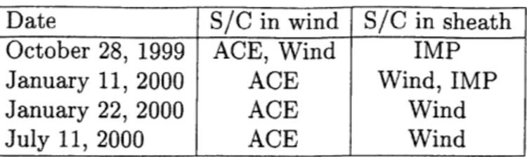
In order to find shock pairs to analyze, I began with an ACE "Lists of Disturbances and Transients" (Smith, 2003) and a list of interplanetary shocks seen by Wind that was compiled by Alan Lazarus (Lazarus and Finck, 2003). I compared the times these shocks were seen to the times that Wind and IMP-8 were supposed to be in the mag-netosheath. The data from ACE, Wind, and IMP-8 were plotted for candidate events using a routine in the IDL programming language. Shocks in the magnetosheath were identified by looking at the surrounding data. In the magnetosheath, the ther-mal speed is elevated, and the east-west flow angle ranges from 5 to 15 degrees due to the deflection induced by Earth's magnetic field. Most of the shocks identified failed to have valid corresponding magnetosheath data, either because the spacecraft was actually in the magnetosphere, because there was too much noise to pick out the shock from the surrounding data, or because the shock compressed the bow shock within the spacecraft's orbit, pushing the spacecraft into the solar wind. I ultimately found four pairs of shocks to analyze (Table 1).

Date S/C in wind S/C in sheath

October 28, 1999 ACE, Wind IMP

January 11, 2000 ACE Wind, IMP January 22, 2000 ACE Wind July 11, 2000 ACE Wind

Table 1: List of interplanetary shocks to be analyzed and which spacecraft saw each shock in the solar wind and in the magnetosheath.

4.2

Shock Analysis

These shocks are analyzed by looking at how their parameters change before and after the shock passes the spacecraft. The "upstream" solar wind data are seen first; they come before the interplanetary shock wave passes the spacecraft and are supersonic in the frame of the shock wave. Then the shock passes, and behind it is seen the "downstream" data which is subsonic in the frame of the shock wave. The shock itself takes barely a second to pass the spacecraft as can be seen in Figure 4. While it is only 103 km thick at 1 AU, it is about 10" km wide and can be treated as a plane wave (Kasper, 2002). The analysis methods characterize the shock by looking at the upstream and downstream data. Figure 4 shows an example of upstream and downstream parameters that were picked to be used for one of the shocks. Using the velocity coplanarity and Rankine-Hugoniot methods of analysis provided by Justin Kasper (Kasper, 2002), I generated two predictions for the direction and speed of each shock seen in the solar wind.

The velocity coplanarity (VC) method of determining the shock normal takes into account only the upstream and downstream velocities, ignoring all other parameters. This is calculated as

Ud -

(1

hVC = -# -' , (1)

jUd - U17

To determine the direction of propagation using the Rankine-Hugoniot (RH) method as developed by Justin Kasper (Kasper, 2002), the upstream and downstream

12 U 10 6 -325 E -345 > -350 -3 -Y -5 10 -1 -20 --3 -X-40 > 50 S-6 x -7 -8 --20 -10 0 10 20 30

Time from event [seconds]

Figure 4: Example of data used in interplanetary shock analysis. From the January 22, 2000 shock seen by ACE. Top to bottom: Proton number density; Bulk velocity components; Magnetic field components. Error bars indicate the uncertainty of the individual measurements, the diamonds mark points selected for further analysis, and the horizontal lines mark the average measurement that was used in the analysis.

where

U

minimum value of X2

, where

C?

X2

(0,5)

=Z

and 9i is the vector of uncertainties of each of the calculated values of C2.

Once the shock normals are known, we can calculate the shock speed. This is derived from the fact that we know by mass conservation thatq the flux across the shock's surface must be the same looking from upstream or downstream . For fluxes of F1 upstream and F2 downstream and corresponding pi and P2 this means that

P2 (2 -h) = P1 (1 - h) (3)

which, in the frame of reference of the shock becomes

P2 (2 -ii - Vs) =-P 1(1 -fi -Vs) (4)

so we find that the speed of the shock is

2 - h - 1 (1 -, .f)

VS =2 (5)

P2

The ratio P is known as the compression ratio of the shock, which is a measure

PI

of how strong the shock is. We can also get a sense of how fast the shock is traveling in the medium by looking at its fast and Alfven mach numbers. These are found by comparing AV = IV2 - 1 to the sound speed and Alfvene speed, respectively.

4.3 Determining Delay

Once the shock normal and shock speed has been determined at the upstream space-craft, it is possible to determine the delay for it to arrive at a downstream spacecraft

based on its location. Given a shock moving at speed V, with the front normal h and two spacecraft separated by a distance d , if dS1 = dS- h then the arrival delay is

dS _-nh

V 8 =

- (6 )

Once this value is known, it can be compared to the actual delay in order to deter-mine if and how the velocity of the shock changes as observed in the magnetosheath.

5

Results: Shocks Seen in Magnetosheath

Only two of the shock pairs evaluated here had analyzable data for the shock when it was seen in the magnetosheath. The other two shocks only provided us with the arrival time of the shock at the spacecraft and will be discussed later. The former two shocks are particularly interesting to look at because not only can we check the predicted arrival time, but it is also possible to find a velocity for the shock itself in the magnetosheath.

5.1 January 11, 2000

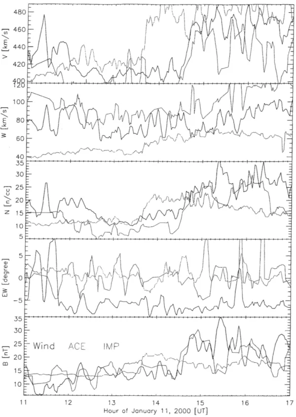
The event seen on January 11, 2000 is an exceptional example since it was seen in the solar wind by ACE, and in the magnetosheath by both Wind and IMP-8 (Figure 5). Moreover, the data recorded in the magnetosheath were analyzable, giving us actual predictions of the shock's velocity as it travels through the magnetosheath. These data are illustrated in Figure 6. The velocity and magnetic field nicely demonstrate the correlation between these events and lead to the conclusion that it is, indeed, the same shock. We can tell that the Wind and IMP-8 spacecraft are in the magnetosheath by their elevated thermal speeds and negative east-west flow angles (i.e. from the East of the Sun). The flow angle indicates the deflection of the wind by Earth's magnetic field.

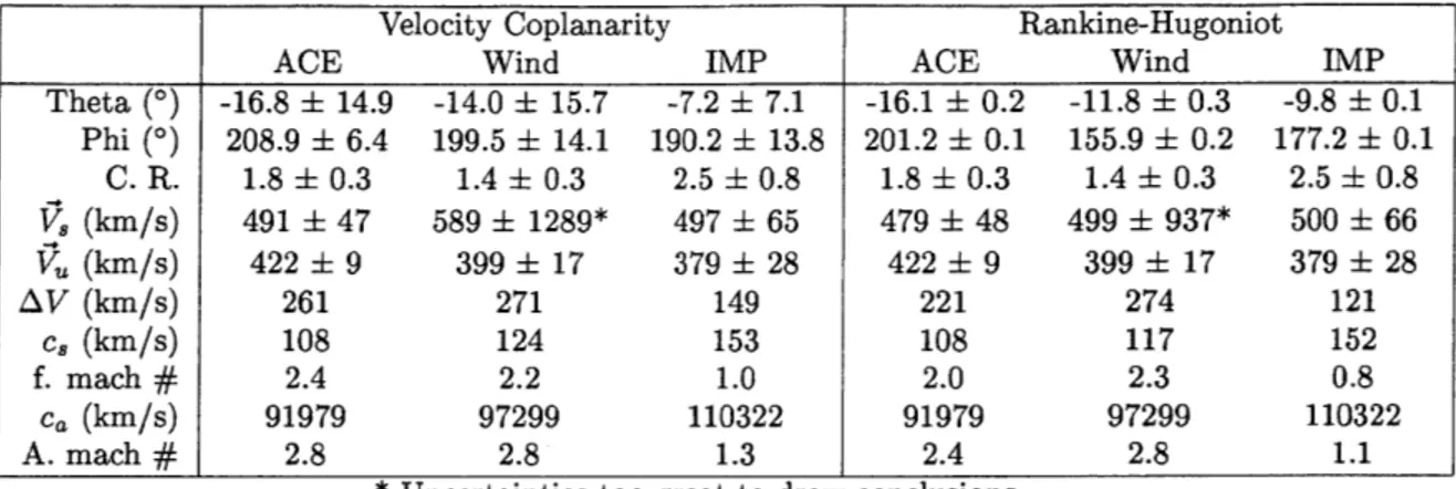
Table 2 lists the speeds of the shock when it reaches each spacecraft as determined

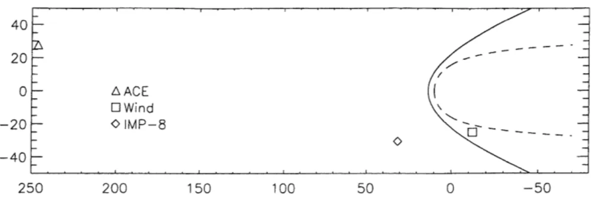
40-20- -0 A ACE OWind -20- oIMP-8 -40-.. . . . . . 250 200 150 100 50 0 -50

Figure 5: Positions of spacecraft when they saw the January 11, 2000 shock. In cylindrical coordinates, with positive/negative based on Y-GSE position.

agree very well and there is no notable slowing of the shock seen in the magnetosheath. Due to the large uncertainty in the Wind measurements, we will have to rely on a comparison between ACE and IMP-8.

The comparison of the predicted delay of the shock as it travels from the solar wind into the magnetosheath can be found in Table 3. We see that the deviation of the actual delay from the predicted delay is well within the uncertainties for both predictions on both spacecraft in the sheath. This and the similarities between the shock speed at ACE and IMP-8 lead to the conclusion that there is no slowing of the shock as it travels through the sheath.

5.2 July 11, 2000

After extensive analysis the event on July 11, 2000, as seen in Figure 7 does not appear to be an interplanetary shock wave, due to the lack of a jump in the magnetic field. It is interesting to consider how the disturbance propagates through the magnetosheath, nonetheless. This disturbance was seen by ACE in the solar wind and IMP-8 in the magnetosheath (Figure 8).

In Table 4 we see that the speed of the disturbance as measured at ACE in the wind and IMP-8 in the sheath are consistent with each other for the velocity coplanarity analysis method. However, looking at the results of the Rankine-Hugoniot analysis, we see a slowing of the shock in the sheath. The actual and predicted delays assuming

480 460 440-420 100-60 --40 35-30 25 20 \ 2 15 10 35 30 25 -Wind ACE MP S20-35 15 10 11 12 13 14 15 16 17

Hour of January 11, 2000 [UT]

Figure 6: Interplanetary shock as seen by ACE in the solar wind, and Wind and IMP-8 in the magnetosheath. Top to bottom: Speed; Thermal speed; Proton number density; East-west flow angle; Magnetic field magnitude.

Velocity Coplanarity Rankine-Hugoniot

ACE Wind IMP ACE Wind IMP

Theta (0) -16.8 14.9 -14.0 15.7 -7.2 7.1 -16.1 0.2 -11.8 0.3 -9.8 i 0.1 Phi (0) 208.9 6.4 199.5 14.1 190.2 13.8 201.2 0.1 155.9 0.2 177.2 t 0.1 C. R. 1.8 +0.3 1.4 0.3 2.5 0.8 1.8 t 0.3 1.4 0.3 2.5 0.8 , (km/s) 491 47 589 1289* 497 65 479 48 499 937* 500 t 66 V, (km/s) 422 9 399 + 17 379 28 422 9 399 17 379 28 AV (km/s) 261 271 149 221 274 121 c, (km/s) 108 124 153 108 117 152 f. mach # 2.4 2.2 1.0 2.0 2.3 0.8 Ca (km/s) 91979 97299 110322 91979 97299 110322 A. mach # 2.8 2.8 1.3 2.4 2.8 1.1

* Uncertainties too great to draw conclusions.

Table 2: Comparison of the parameters of the January 11th shock as calculated by the velocity coplanarity and Rankine-Hugoniot methods when seen at ACE in the solar wind and Wind and IMP-8 in the magnetosheath. Top to bottom: Angle out of ecliptic; Angle in ecliptic; Compression ratio; Shock speed; Upstream speed; Speed difference; Sound speed; Fast mach number; Alfven speed; Alfven mach number.

ACE-Wind ACE-IMP

Actual VC RH Actual VC RH

Delay 3181 3365 3305 3256 3236 3391

Uncertainty 253 317 288 181

Difference from actual +184 +124 -20 +136

Table 3: Comparison of velocity coplanarity and Rankine-Hugoniot predictions of delay of January 11th shock propagating at constant velocity from ACE in the solar wind, to Wind and IMP-8 in the magnetosheath, to the actual delay in seconds.

480 460 J\ 440 40 380 360 340. .1U -100 -30 - E-40 - -20 50-30 25 0 -Q)-5 )-10 - -15--20 -30 25-207- WindAE 15-10 -6 -4 -20 2 4

Hour of July 11, 2000 [UT]

Figure 7: Interplanetary shock as seen by ACE in the solar wind, and Wind in the magnetosheath. Top to bottom: Speed; Thermal speed; Proton number density; East-west flow angle; Magnetic field magnitude.

40_ 20 0 A ACE El Wind -20 0 IMP-8 -40 250 200 150 100 50 0 -50

Figure 8: Positions of spacecraft when they saw the July 11, 2000 shock. In cylindrical coordinates, with positive/negative based on Y-GSE position.

constant speed are shown in Table 5. Here we clearly see that the Rankine-Hugoniot method produces a valid prediction, whereas the velocity coplanarity method which neglected the magnetic field does not.

6

Results: Shocks Passing into Magnetosheath

The other two shocks that are discussed here were not analyzable in the magne-tosheath. This is due to the fact that they were not directly observed. Instead, we see the spacecraft pass from the magnetosphere into the magnetosheath at the time of the shock's arrival. This is due to the fact that as the shock passes it compresses the magnetopause, essentially "popping" the spacecraft out of the magnetosphere at the time of its arrival.

6.1 October 28, 1999

This type of event occurred on October 28, 1999 while IMP-8 was in the magne-tosheath (Figure 9). We see in Figure 10 that there is only sporadic data from IMP-8 while it is in the magnetosphere due to the very low density in this region. Then when it is pushed into the magnetosheath, the density and thermal speed jump, and it is this occurrence that marks the passing of the shock.

giv-Table 4: Comparison of the parameters of the July 11th shock as velocity coplanarity and Rankine-Hugoniot methods when seen at wind and Wind in the magnetosheath. Top to bottom: Angle out in ecliptic; Compression ratio; Shock speed; Upstream speed; Speed speed; Fast mach number; Alfven speed; Alfven mach number.

5: of to

calculated by the ACE in the solar of ecliptic; Angle difference; Sound ACE-Wind Actual VC RH Delay 2628 4007 2693 Uncertainty 158 167

Difference from actual +1378 +64

Comparison of velocity coplanarity and Rankine-Hugoniot predictions of July 11th shock propagating at constant velocity from ACE in the solar Wind in the magnetosheath, to the actual delay in seconds.

40-20 A-0 AACE 0 Wind -20 - IMP-8 -40 250 Figure 9: cylindrical 200 150 100 50 0 -50

Positions of spacecraft when they saw the October 28, 1999 shock. In coordinates, with positive/negative based on Y-GSE position.

Velocity Coplanarity Rankine-Hugoniot

ACE Wind ACE Wind

Theta (0) -20.0 4 9.5 -9.6 5.2 2.9 0.1 66.2 t 0.2 Phi (0) 219.7 t 6.3 211.1 2.8 126.8 0.1 201.8 0.6 C. R. 1.9 0.2 2.8 0.4 1.9 0.2 2.8 0.4 V (km/s) 433 26 482 17 247 13 159 7 V, (km/s) 425 8 346 12 425 8 346 12 AV (km/s) 331 175 149 324 cS (km/s) 104 186 107 191 f. mach # 3.2 0.9 3.1 1.7 Ca (km/s) 98961 179673 98961 179673 A. mach # 3.3 1.0 3.4 1.8 Table delay wind,

440 420 400 E 380 360 320 80 80-E 60-40 .

25-20- Wind ACE IMP

15 10 -0 . . .. .... 0 5 S 0 j -5 -10 . 1 1 10 F- 9 7 6 8 9 10 1 1 12 13 14 15

Hour of October 28, 1999 [UT]

Figure 10: Interplanetary shock as seen by ACE and Wind in the solar wind, and IMP-8 in the magnetosheath. Top to bottom: Speed; Thermal speed; Proton number density; East-west flow angle; Magnetic field magnitude.

ACE-IMP Wind-IMP

Actual VC RH Actual VC RH

Delay 3271 3440 3455 552 501 488

Uncertainty 335 269 353 220 Difference from actual +170 +184 -51 -63

Table 6: Comparison of velocity coplanarity and Rankine-Hugoniot predictions of delay of October 28th shock propagating at constant velocity from ACE and Wind in the solar wind, to IMP-8 in the magnetosheath, to the actual delay in seconds.

ACE-Wind

Actual VC RH

Delay 3394 3213 2926

Uncertainty 955 1364 Difference from actual -180 -468

Table 7: Comparison of velocity coplanarity and Rankine-Hugoniot predictions of delay of January 22nd shock propagating at constant velocity from ACE in the solar wind, to Wind in the magnetosheath, to the actual delay in seconds.

ing us two propagation delay predictions to consider. The outcome of the comparison of the delay predicted by our methods to the actual delay is shown in Table 6. Again we see that the difference between the predicted and actual delays are within the uncertainties of the predictions, providing further evidence of interplanetary shock waves' constant speed in the magnetosheath.

6.2 January 22, 2000

Again on January 22, 2000 a shock comes along and pushes a spacecraft, in this case Wind, out of the magnetosphere into the magnetosheath by compressing the magnetopause (Figure 11). In this case, due to the sensitivities of Wind's instruments, we saw no data while Wind is in the magnetosphere (Figure 12).

Table 7 shows the predicted propagation delays for this shock as it travels from

ACE to Wind. We see here that the actual delays are very close to the predictions,

despite their large uncertainties. This agrees with the assessment that their is no slowing of the shock in the magnetosheath.

40-20 0- A ACE - 2 Wind -20 - 0 IMP-8 -40~ 250 200 150 100 50 0 -50

Figure 11: Positions of spacecraft when they saw the January 22, 2000 shock. In cylindrical coordinates, with positive/negative based on Y-GSE position.

7

Conclusion

Here we have examined four interplanetary shock waves and disturbances in the solar wind and attempted to assess their propagation speed as they pass through the magnetosheath. Three of the four supported the assertion that there is no slowing of these events as they pass through the magnetosheath. The fourth, which is indeed not an actual shock wave, shows some slowing when considered using a method that

accounts for its uncharacteristic magnetic field.

The shock wave seen on January 11, 2000 lends support to the idea that the speed remains unchanged. For here we were able to analyze the shock in the magnetosheath as we would in the solar wind and found that the velocity was consistent with the shock data when seen in the solar wind. Thus we conclude that while interplanetary shocks are deflected when they pass through the bow shock, there is no substantial modification to their speeds. This result disagrees with that of Villante et al. (2003).

440 420 r 400 E 380 360 - 340-

320".-88

Hour of January 22, 2000 [UT]

Figure 12: Interplanetary shock as seen by ACE in the solar wind, and Wind in the magnetosheath. Top to bottom: Speed; Thermal speed; Proton number density; East-west flow angle; Magnetic field magnitude.

Bibliography

Acufna, M. H., Ogilve, K. W., Baker, D. N., Curtis, S. A., Fairfield, D. H., and Mish, W. H. (1995). The global geospace science program and its investigations. In Russell, C. T., editor, The Global Geospace Mission, pages 5-21. Kluwer Academic Publishers.

Christian, E. R. and Davis, A. J. (2002). Advanced composition explorer (ace) mission

overview. Website. http: //www.sri. caltech. edu/ACE/ace-mission.html.

Kasper, J. C. (2002). Properties of Collisionless Shocks. PhD thesis, Massachusetts

Institute of Technology.

Kivelson, M. G. and Russell, C. T. (1995). Introduction to Space Physics. Cambridge University Press.

Lazarus, A. J. and Finck, L. A. (2003). Wind events. Website.

ftp: //space.mit.edu/pub/plasma/wind/wind- events/windevents, text.

McComas, S. J., Barker, P., Feldman, W. C., Phillips, J. L., and Riley, P. (1998). Solar wind electron proton alpha monitor (swepam) for the advanced composition explorer. Space Science Reviews, 86. Special Issue on the ACE Mission.

Ogilve, K. W., Chornay, R. J., and Fritzenreiter, R. J. e. a. (1995). Swe, a compre-hensive plasma instrument for the wind spacecraft. In Russell, C. T., editor, The

Global Geospace Mission, pages 5-21. Kluwer Academic Publishers.

Rasinkangas, R. (1999). Solar wind & interplanetary magnetic field (imf). In Oulu Space Physics Textbook. Space Physics Group of Oulu. http: //www. oulu. fi/spaceweb/textbook/solarwind. html.

Smith, C. W. (2001). Ace/mag project - mag instrument. Website. http://www.bartol.udel.edu/-chuck/ace/instrument.html.

Smith, C. W. (2003). Ace lists of disturbances and transients. http://ww.bartol.udel.edu/~chuck/ace/ACElists/obs.list.html.

Villante, U., Lepidi, S., Francia, P., and Bruno, T. (2003). Some aspects of the interaction of interplanetary shocks with the earth's magnetosphere: an estimate of the propogation time through the magnetosheath. In press for J. Atm. Terr.