THE EXOPLANET SYSTEMS KEPLER-50 AND KEPLER-65
The MIT Faculty has made this article openly available. Please share
how this access benefits you. Your story matters.
Citation Chaplin, W. J., R. Sanchis-Ojeda, T. L. Campante, R. Handberg, D. Stello, J. N. Winn, S. Basu, et al. “ASTEROSEISMIC DETERMINATION OF OBLIQUITIES OF THE EXOPLANET SYSTEMS KEPLER-50 AND KEPLER-65.” The Astrophysical Journal 766, no. 2 (March 14, 2013): 101.
As Published http://dx.doi.org/10.1088/0004-637x/766/2/101
Publisher IOP Publishing
Version Author's final manuscript
Citable link http://hdl.handle.net/1721.1/89201
Terms of Use Creative Commons Attribution-Noncommercial-Share Alike
arXiv:1302.3728v1 [astro-ph.EP] 15 Feb 2013
W. J. Chaplin1, R. Sanchis-Ojeda2, T. L. Campante1, R. Handberg3, D. Stello4,
J. N. Winn2, S. Basu5, J. Christensen-Dalsgaard3, G. R. Davies1, T. S. Metcalfe6,
L. A. Buchhave7,8, D. A. Fischer5, T. R. Bedding4, W. D. Cochran9, Y. Elsworth1,
R. L. Gilliland10, S. Hekker11,1, D. Huber12, H. Isaacson13, C. Karoff3, S. D. Kawaler14,
H. Kjeldsen3, D. W. Latham15, M. N. Lund3, M. Lundkvist3, G. W. Marcy13, A. Miglio1,
T. Barclay12,16, J. J. Lissauer12
ABSTRACT
Results on the obliquity of exoplanet host stars – the angle between the stellar spin axis and the planetary orbital axis – provide important diagnostic 1School of Physics and Astronomy, University of Birmingham, Edgbaston, Birmingham, B15 2TT, UK 2Department of Physics, Massachusetts Institute of Technology, 77 Massachusetts Avenue, Cambridge, Massachusetts 02139, USA
3Stellar Astrophysics Centre (SAC), Department of Physics and Astronomy, Aarhus University, Ny Munkegade 120, DK-8000 Aarhus C, Denmark
4Sydney Institute for Astronomy, School of Physics, University of Sydney, Sydney, Australia 5Department and Astronomy, Yale University, New Haven, CT, 06520, USA
6White Dwarf Research Corporation, Boulder, CO, 80301, USA
7Niels Bohr Institute, Copenhagen University, DK-2100 Copenhagen, Denmark
8Centre for Star and Planet Formation, Natural History Museum of Denmark, University of Copenhagen, DK-1530 Copenhagen, Denmark
9McDonald Observatory, The University of Texas, Austin, TX 78712, USA
10Center for Exoplanets and Habitable Worlds, The Pennsylvania State University, University Park, PA, 16802, USA
11Astronomical Institute, “Anton Pannekoek”, University of Amsterdam, The Netherlands 12NASA Ames Research Center, MS 244-30, Moffett Field, CA 94035, USA
13Department of Astronomy, University of California, Berkeley, CA 94720, USA 14Department of Physics and Astronomy, Iowa State University, Ames, IA, 50011, USA 15Harvard-Smithsonian Center for Astrophysics, Cambridge, Massachusetts 02138, USA 16
information for theories describing planetary formation. Here we present the first application of asteroseismology to the problem of stellar obliquity determination in systems with transiting planets and Sun-like host stars. We consider two systems observed by the NASA Kepler Mission which have multiple transiting small (super-Earth sized) planets: the previously reported Kepler-50 and a new system, Kepler-65, whose planets we validate in this paper. Both stars show rich spectra of solar-like oscillations. From the asteroseismic analysis we find that each host has its rotation axis nearly perpendicular to the line of sight with the sines of the angles constrained at the 1σ level to lie above 0.97 and 0.91, respectively. We use statistical arguments to show that coplanar orbits are favoured in both systems, and that the orientations of the planetary orbits and the stellar rotation axis are correlated.
Subject headings: asteroseismology — stars: rotation — planets and satellites: formation — planets and satellites: general
1. Introduction
The obliquities of the host stars in exoplanetary systems display a surprising diversity, including low obliquities reminiscent of the solar system, strongly tilted stars, and retro-grade systems in which the directions of stellar rotation and planetary orbital revolution are opposite. Most of these results have been obtained by detecting the Rossiter-McLaughlin (RM) effect, a spectroscopic anomaly that is observed during a planetary transit (Queloz et al. 2000, Winn et al. 2005). In addition, for some systems the obliquity has been determined through the detection and interpretation of transits of a planet over starspots (e.g., Deming et al. 2011, D´esert et al. 2011, Nutzman et al. 2011, Sanchis-Ojeda et al. 2011), and for one system (Barnes et al. 2011, Szab´o et al. 2011) it has been estimated using the signatures of gravity darkening from rapid stellar rotation (Barnes 2009).
Almost all of the previous results pertain to host stars with hot Jupiters. The diversity of obliquities seen in those systems has been taken as evidence that the process of converting a “normal” Jupiter into a hot Jupiter can tilt the inclination of the planetary orbit (see, e.g., Winn et al. 2010a, Triaud et al. 2010, Albrecht et al. 2012). It would be interesting to extend these measurements to systems with longer-period planets, and multiple-planet systems, to test whether the high obliquities are indeed confined to the hot Jupiter systems. Unfortunately, the long-period and multiple-planet systems tend to involve smaller planets and intrinsically fainter host stars (Latham et al. 2011, Steffen et al. 2012), making it difficult to apply the RM and starspot techniques. This is why only two such systems have been
examined to date (Sanchis-Ojeda et al. 2012, Hirano et al. 2012b). It would be advantageous to develop a technique that does not depend so critically on the signal-to-noise ratio of the transit data. One possibility is to use a combination of the measured rotation period (Prot),
the projected rotation rate (v sin is) and the stellar radius (R) to determine sin is, the sine
of the angle is between the stellar rotation axis and the line of sight (see, e.g., Hirano et al.
2012a). However, this method is usually limited by the relatively poor accuracy of v sin is
measurements for cool stars.
Asteroseismology provides another potentially powerful method. The detection and interpretation of the solar-like oscillations shown by solar-type stars is well known to provide accurate fundamental properties of host stars (e.g., Bazot et al. 2005, Bouchy et al. 2005, Vauclair et al. 2008, Soriano & Vauclair 2010, Christensen-Dalsgaard et al. 2010, Ballot et al. 2011, Batalha et al. 2011, Gilliland et al. 2011, Howell et al. 2011, Borucki et al. 2012, Carter et al. 2012, Escobar et al. 2012, Barclay et al. 2013). Less well known is that in some cases the rotationally-induced splittings of oscillation modes can be used to determine is
(Gizon & Solanki 2003). When the host star also has a transiting planet, the inclination ip
of the planetary orbit can be determined, and therefore the difference in inclination between the star and planetary orbit can be calculated.
In contrast to the RM and starspot techniques, the applicability of the asteroseismic method depends predominantly on the stellar parameters and hardly at all on the planetary parameters, giving the asteroseismic method a decisive advantage in measuring the stellar obliquities in systems with small planets or long-period planets. The asteroseismic analysis does, however, require bright targets and long-duration, high-cadence photometric time series to give the requisite signal-to-noise and frequency resolution for extracting clear signatures of rotation from the oscillation spectrum, and hence the stellar inclination angle.
Here we present the first application of asteroseismology to the problem of stellar obliq-uity determination for Sun-like exoplanet hosts with transiting planets. Both of the sys-tems considered in this paper have solar-type stars hosting multiple, small (super-Earth sized) transiting planets. The identification of the two-planet Kepler-50 system (KOI-262, KIC 11807274), along with the validation of the transit signals as arising from planets, was previously reported by Steffen et al. (2013). Kepler-65 (KOI-85, KIC 5866724) is a three-planet system that is herein identified and validated for the first time. Both systems involve F-type stars at the brighter end of the Kepler target list, having apparent magnitudes of Kp = 10.42 and Kp = 11.02, respectively.
Previously, asteroseismic methods have been applied to host stars with single, non-transiting large planets discovered using the Doppler method – HD 52265, a solar-type host with asteroseismic data from CoRoT (Ballot et al. 2011; and HR 8799, an A-type host
showing γ Doradus pulsations in ground-based observations (Wright et al. 2011) – with only moderate constraints returned on the stellar inclinations.
The rest of the paper is organized as follows. We begin in Section 2 by estimating the fundamental stellar properties, using the solar-like oscillations detected in the Kepler lightcurves and complementary spectroscopic data. Section 3 presents the planet properties of both systems, including validation of the planets orbiting Kepler-65 and discussion of the mutual inclinations of the planetary orbits of both systems. The asteroseismic estimation of the stellar obliquities, which depends on extracting signatures of rotation from the oscillation spectra, is presented in Section 4. Section 5 compares the asteroseismic results on rotation with independent estimates of the surface rotation based on the quasi-periodic variations seen in the Kepler lightcurves, and measurements of the sky-projected surface rotational velocity based on spectroscopic line broadening. We finish in Section 6 with a discussion of the implications of our results for theories of planetary formation.
2. Fundamental properties of the stars
We determined the fundamental stellar properties of Kepler-50 and Kepler-65 by com-paring a few key asteroseismic and spectroscopic observables to the outputs of stellar-evolutionary models.
The asteroseismic results are based on the Kepler short-cadence (SC) data (Gilliland et al. 2010), whose one-minute sampling is needed to detect the short-period oscillations observed in solar-type stars (see also Chaplin et al. 2011a). The lightcurve for Kepler-50 spans 18 months, from Kepler observing quarters 6 through 11 inclusive. The lightcurve for Kepler-65 spans 27 months, from quarters 3 through 11.
Before computing power spectra, the planetary transit signals were removed from the time series by applying a median high-pass filter of width appropriate for the transit durations (see, e.g., Christensen-Dalsgaard et al. 2010). The clear separation of the relevant timescales – i.e., periods of days associated with the transits versus periods of minutes associated with the dominant oscillations – means that this approach cleans the frequency-power spectrum in such a way as to allow the asteroseismic analysis to proceed unhindered. Fig. 1 shows frequency-power spectra of the lightcurves of Kepler-50 (top panel) and Kepler-65 (bottom panel). The spectra were computed using a Lomb-Scargle periodogram (Scargle 1982), and calibrated to satisfy Parseval’s theorem. Both stars present clear patterns of peaks due to solar-like oscillations, which are small-amplitude pulsations that are stochastically excited and intrinsically damped by the near-surface convection. Many acoustic (pressure, or p)
modes of high radial order, n, are excited to observable amplitudes. Solar-type stars oscillate in both radial and non-radial modes. The modes may be decomposed onto spherical harmonic functions of degree l. Both stars show detectable overtones of modes with l ≤ 2.
2.1. Spectroscopic data and analysis
Estimates of Teff and [Fe/H] were obtained by analyzing high-resolution optical spectra.
The observations were made as part of the Kepler Follow-up Observing Program (KFOP). Spectra were collected for both stars using the HIRES spectograph on the 10-m Keck tele-scope on Mauna Kea. In the case of Kepler-50 spectra were also collected with the fiber-fed Tillinghast Reflector Echelle Spectrograph (TRES) on the 1.5-m Tillinghast Reflector at the Fred Lawrence Whipple Observatory, and the Tull Coud´e Spectrograph on the 2.7-m Harlan J. Smith Telescope at the McDonald Observatory, Texas. For Kepler-65, additional spectra were collected by the FIber-fed Echelle Spectrograph (FIES) on the 2.5-m Nordic Optical Telescope (NOT) on La Palma.
The Keck data were analyzed using the Spectroscopy Made Easy (SME) pipeline (Valenti & Piskunov 1996; Valenti & Fischer 2005). Data from the other telescopes were analyzed with the Stellar Parameter Classification (SPC) pipeline (Buchhave et al. 2012). Good agree-ment was found between the SME and SPC estimates of Teff and [Fe/H]. For subsequent
analysis we adopted the SME values. The SME and SPC analyses also provided estimates of v sin i based on the observed line broadening (see Torres et al. 2012 for further details). Section 5 discusses the comparison of those results with the asteroseismic estimates of stellar rotation rates.
A well-known problem with the analysis of high-resolution spectra of solar-type stars is that log g is difficult to pin down, and subject to systematic errors that propagate into the uncertainties of other parameters such as Teff and [Fe/H]. For this reason, an iterative
procedure was used to refine the estimates of the spectroscopic parameters (e.g., see Bruntt et al. 2012, Torres et al. 2012). In this procedure, the initial values of the spectroscopic parameters are used together with the asteroseismic parameters to compute log g (see next section). The spectroscopic analysis was then repeated with log g fixed at this asteroseismic value, to yield the revised values of Teff and [Fe/H]. Convergence of the inferred properties
(to within the estimated uncertainties) was achieved after just a single iteration. The final, iterated spectroscopic results are presented in Table 1.
Fig. 1.— Frequency-power spectra of Kepler-50 (top panel) and Kepler-65 (bottom panel), showing rich spectra of overtones of solar-like oscillations. The main plots in both figures show six overtones, with modes tagged according to their angular degree, l. The so-called large frequency separation between one pair of adjacent l = 0 modes is also marked. The insets show the full frequency extent of both observable p-mode spectra. The Gaussian-like power envelope of each spectrum is readily apparent, which peaks at νmax. Plots rendered
in black are the power spectra after smoothing with a 1.5µHz filter. The light grey curves show the spectra after applying lighter smoothing.
2.2. Asteroseismic estimation of stellar properties
A two-stage procedure was adopted to estimate the fundamental properties of the stars, using as input asteroseismic parameters and complementary spectroscopic results. At the first stage for each star we sought initial estimates of the stellar properties by searching among grids of stellar evolutionary models to get a best fit to two global oscillation prop-erties, the spectroscopically estimated effective temperature Teff, and metallicity, [Fe/H].
The two asteroseismic properties were h∆νi, the average of the large frequency separations between consecutive overtones n of the same angular degree l; and νmax, the frequency of
maximum oscillation power. The average large separations scale to very good approximation as hρi1/2, where hρi ∝ M/R3 is the mean density of the star with mass M and surface radius
R (see, e.g., Christensen-Dalsgaard 1993). The frequency of maximum oscillation power has been shown to scale to good approximation as gTeff−1/2 (Brown et al. 1991; Kjeldsen & Bedding 1995; Belkacem et al. 2011), where g is the surface gravity. Several analysis codes (Christensen-Dalsgaard et al. 2010; Hekker et al. 2010; Huber et al. 2009; Verner et al. 2011) were applied to the frequency-power spectra to extract the required estimates. A final value of each parameter was selected by taking the individual estimate that lay closest to the me-dian. The uncertainty on the final value was given by adding (in quadrature) the uncertainty on the chosen estimate and the standard deviation over the set of results. For Kepler-50 we obtained h∆νi = 76.0 ± 0.9 µHz and νmax = 1496 ± 56 µHz; while for Kepler-65 we obtained
h∆νi = 90.0 ± 0.5 µHz and νmax= 1880 ± 60 µHz.
The grid-based search codes that we then applied to these results are described by Stello et al. (2009), Basu et al. (2010), Quirion et al. (2010) and Gai et al. (2011).
In the second stage we used estimates of the individual oscillation frequencies, along with the revised spectroscopic data, as inputs to a detailed modelling performed by three members of the team (SB, JCD and TM). The procedure used to estimate the frequencies – which also provided information on the internal rotation and angle of inclination of each star – is discussed in detail in Section 4. More details on the detailed modeling used to estimate the stellar properties is given in the Appendix, which followed the methodology applied in, for example, Christensen-Dalsgaard et al. (2010), Howell et al. (2011) and Carter et al. (2012). Estimated properties from the first, grid-based stage were used either as starting guesses or as a guideline check for initial results. The final properties presented in Table 1 come from the analysis made by JCD (which provided the median solutions). Uncertainties on the final properties include a contribution from the scatter between the three different sets of results. We note that the properties from the first stage showed excellent agreement with the final estimated properties (i.e., to within the estimated uncertainties).
3. Characterization of the planetary systems
It is important to establish whether the transit-like photometric signals represent actual transits of a system of planets across the disk of the intended target star, as opposed to a “false positive” such as a system of eclipsing stars blended with the intended target star. For Kepler-50, transit timing variations (TTV) have been observed for both of its planets and are anti-correlated, a clear sign that the planets are interacting with each other and hence orbit the same star (Steffen et al. 2013). Kepler-65 has not been confirmed in this manner; in the following section we validate the system by other means.
3.1. Validation of Kepler-65
To validate the Kepler-65 system, in this section we will demonstrate that: (i) back-ground eclipsing binaries are unlikely to be responsible for any of the three candidate transit signals; (ii) all three transiting objects are likely orbiting the same star, which must have a mean density very similar to that of the intended target star; and (iii) planets c and d are near a 7:5 mean-motion commensurability, and the smaller planet in this pair (planet d) exhibits a significant TTV signal of the nature expected for such a configuration.
3.1.1. Excluding background binary scenarios
Lissauer et al. (2012) considered the question of how many of Kepler ’s multiple-planet candidates actually represent true multiple-planet systems, as opposed to unresolved blends of systems each having only one eclipsing object. For example, a candidate two-planet system could actually be a single-planet system along nearly the same line of sight to a background eclipsing binary, or there could be two eclipsing binaries along the same line of sight whose eclipses are diluted to planet-like proportions by the constant light of a foreground star. Lissauer et al. (2012) recognized that false positives of this nature would be randomly dis-tributed among the target stars, and that the number of multiple-planet candidates is much
Table 1. Estimated stellar properties
Star Teff [Fe/H] M R hρi log g Age
(K) (dex) (M⊙) (R⊙) (g cm−3) (dex) (Gyr)
Kepler-50 6225 ± 66 0.03 ± 0.06 1.24 ± 0.05 1.58 ± 0.02 0.441 ± 0.004 4.132 ± 0.005 3.8 ± 0.8 Kepler-65 6211 ± 66 0.17 ± 0.06 1.25 ± 0.06 1.41 ± 0.03 0.621 ± 0.011 4.232 ± 0.006 2.9 ± 0.7
larger than would be expected if the candidates were assigned randomly to target stars. From this analysis they concluded that the vast majority of Kepler ’s multiple-planet candidates do not represent superpositions of singly-eclipsing systems. For the population of three-transit candidates such as Kepler-65, Lissauer et al. (2012) estimated the chance that at least one of the candidates represents an unrelated eclipsing system is 0.07% (an expectation of 0.13 such false positives out of 178 candidates).
These general considerations show that Kepler-65 is very likely a true multiple-planet system, as opposed to unrelated singly-eclipsing systems that are blended together in the
Kepler photometric aperture. In the remainder of this section we examine the specific circumstances and follow-up observations of Kepler-65 that also support this conclusion.
The photometric aperture used for the star changes from quarter to quarter, but in all cases has a size of approximately 4 × 4 pixels. With a detector scale of 3.98 arcsec pixel−1,
stars within a radius of about 12 arcsec from Kepler-65 could contribute light to the aperture and could in principle be the source of some of the transiting signals. We checked for possible contaminating stars using two different datasets.
Firstly, we consulted the catalog by Adams et al. (2012) of adaptive optics (AO) images of a large sample of KOIs. The range of star magnitudes that can be detected depends on the distance to the star, such that one loses the ability to detect faint stars very close to the main star. These images have a range of 6 arcsec, outside of which no information was provided1 Only one other star was detected on the AO image, at a separation of 2.9 arcsec
from Kepler-65. Adams et al. (2012) estimated that the Kepler apparent magnitude of this star is Kp ≈ 21, i.e., about 10 magnitudes fainter than Kepler-65.
Secondly, to seek companions outside the 6 arcsec radius, we consulted the Naval Ob-servatory Merged Astrometric Dataset (Zacharias et al. 2004). In this catalog, 11 stars are detected within a box of 30 arcsec centered on the position of Kepler-65. Only three stars were found that could be candidates for a background blend; one at a separation of 7.2 arcsec with an R-band magnitude of 18.6 (compared to 10.5 for Kepler-65), a second star at a sep-aration of 11.5 arcsec with an R-band magnitude of 14.1, and a third star at a sepsep-aration of 11.8 arcsec with a B-band magnitude of 19.3 (11.6 for Kepler-65).
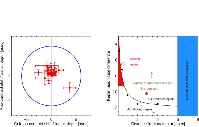
If one of these objects were a background binary star mimicking a transiting planet, then the spatial, first-moment centroid of the light gathered on the aperture would be displaced during eclipses by an amount approximately equal to the observed transit depth multiplied by the projected distance from the object to Kepler-65. Therefore, since the transit depth
−5 0 5 Column centroid shift / transit depth [asec] −5
0 5
Row centroid shift / transit depth [asec]
2 4 6 8
Distance from main star [asec] 12
10 8 6 4
Kepler magnitude difference
Star detected
AO excluded region AO allowed region
Allowed region
Centroid shift excluded region
Brightness ratio allowed region
Fig. 2.— Left-hand panel: Centroid shifts during transits divided by the transit depth for each candidate during each SC quarter. This is an estimate of the distance between the source of the transit signal and the center of light of the system. Based on these data the transit signal must originate from within a 6 arcsec radius (blue circle; see text). Right-hand panel: parameter space for the possible blend scenarios. Plotted on the abscissa is the distance from the center of light in the aperture, and on the ordinate the difference in magnitude with respect to Kepler-65. In addition to the centroid-shift-excluded region (blue), any star just over 9 magnitudes fainter than Kepler-65 is excluded because it would not contribute enough light on the aperture to produce the observed transit depths. This limit is marked by the horizontal dotted line, which was computed assuming an eclipse depth of 50 %. The AO imaging excludes the region above the continuous black line, which was obtained by extrapolation of a best-fitting hyperbolic function, fitted to the limits (black dots) given in Table 2 of Adams et al. (2012). Only the red region is still allowed; in this sense the “radius of confusion” is 0.7 arcsec.
is known independently with high precision, an upper bound on the centroid displacement can be used to set a maximum distance at which a contaminating binary can be located (also known as the radius of confusion). This notion has been applied to detect background binaries among the KOIs (see, e.g., Batalha et al. 2010), to estimate false alarm probabilities (FAPs) for particular KOIs (Morton & Johnson 2011) and to validate individual candidates using the BLENDER technique (Torres et al. 2011).
In the case of Kepler-65, one pixel of the stellar image is saturated, and consequently the distribution of light does not follow the standard point-spread function. Rather than attempting to model the saturated point-spread function, we used the flux-weighted col-umn and row centroids produced by the Kepler pipeline. With this method of computing centroids we are only sensitive to displacements larger than ≈1 pixel (≈4 arcsec), but this is sufficient for our purpose. For each transit observed at short cadence (SC), we selected a window in time of width 4.8 hr centered on each transit. Transits that occurred within 6 hr of another were excluded. To eliminate the effects of outliers we omitted data points differing by more than 3σ from a median-smoothed version of the time series, where the smoothing was performed over 30-min intervals. We found that the centroid motion was approximately a linear function of time, presumably because of the continuous pointing drift of the telescope. We corrected for this effect by fitting the out-of-transit portions of the dataset with a linear function of time. All the centroid information for each candidate in a given quarter was then phase-folded using a linear transit ephemeris from the KOI input catalog (Batalha et al. 2012). The sequences of in-transit and out-of-transit centroids were approximated as Gaussian distributions, and the centroid displacement was computed as the difference between the means of the distributions, with an uncertainty based on standard error propagation.
The left-hand panel of Fig. 2 shows the measured centroid displacements after dividing by the corresponding transit depths, so that implied physical distances are plotted. The signals cannot originate from a source outside the 6 arcsec radius (shown in blue) since no points lie outside that range. The right-hand panel of Fig. 2 shows this constraint, in combination with constraints from other considerations, which together limit the radius of confusion to 0.7 arcsec. One constraint is the AO imaging described previously. Another is that binary stars just over 9 magnitudes fainter than Kepler-65 cannot decrease the total amount of light by 100 ppm (the depth of the shallowest transit), even were they to have eclipses of 50 % depth, i.e., as given by ∆Kp = −2.5 log10[100 × 10−6/ 0.5] ≃ 9.2. This
limit is marked as the horizontal dotted line in right-hand panel of Fig. 2. No stars brighter than that limit and within 0.7 to 6 arcsec from Kepler-65 were detected within the AO image. With such a small radius of confusion, the probability that any of the signals come from background binaries is small. We estimate this probability to be ≤0.15 % for each
candidate of Kepler-65, based on the work by Morton & Johnson (2011), who calculated the local surface density of eclipsing binaries whose properties could mimic those of each
Kepler candidate. Specifically we took their estimated false-positive probability of ≤1 %, which assumed a radius of confusion of 2 arcsec, and scaled it by (0.7/2.0)2 (because we have
demonstrated that the true radius of confusion for Kepler-65 is 0.7 arcsec).
Finally there is the “multiplicity boost,” as discussed at the beginning of this section. Since there are three transit candidates for a single Kepler target, the false alarm probability of each individual transiting object is further reduced, according to the statistical argument of Lissauer et al. (2012). Here the boost factor is approximately 50, which would reduce the individual false-positive probabilities from ≤0.15% to ≤3 × 10⁻⁵.
3.1.2. Evidence that the three planets orbit Kepler-65
We have demonstrated that it is unlikely that any of the transit candidates arises from a background eclipsing binary. We next ask whether the signals represent three planets all orbiting the intended target star Kepler-65, or whether any of them could actually be orbiting a companion star that is gravitationally bound to it. To address this question we searched for a pattern in the transit observables that would suggest that all the planets orbit the same star; namely, transit durations scaling as the cube root of the orbital period, which is a sign that they transit a star with similar density (see, e.g., Fabrycky et al. 2012, Lissauer et al. 2012). If some of the transit signals represented transits across a different star, then such a pattern would occur only by coincidence.
To measure transit durations, we constructed phase-folded transit light curves for each of the three candidates using the SC data and assuming a constant orbital period. Transits that occurred within 6 hr of another were excluded, removing all possible overlapping transits. The data were binned into 7.5-sec intervals to increase the speed of subsequent computations. We used a standard description of the loss of light due to a transiting planet (Mandel & Agol 2002) to model the binned light curves simultaneously. We adopted a quadratic limb-darkening law, with the two coefficients left as free parameters (and shared by all three candidates). The free parameters describing each light curve were the squared planet-to-star radius ratio (Rp/R)2, the impact parameter, b, and the stellar radius divided by the
orbital distance, R/a. We then found the best-fitting model parameters that minimized the standard χ2 function, with uncertainties on the measurements defined as the standard
deviation of the points outside transit for each of the folded light curves. A Markov Chain Monte Carlo (MCMC) code was then used to explore the range of allowed parameters.
From the best-fitting model parameters we computed the transit durations, defined as the interval over which the center of the planet is projected in front of the stellar disk. This parameter is generally well constrained, and does not change much in the presence of a small TTV signal (whereas the ingress duration would experience larger fractional variations). The transit durations are plotted in Fig. 3, as a function of orbital period. We compared these values with those expected for planets in circular orbits around a star with a mean density equal to 0.621 g cm−3, which is the mean density of Kepler-65 as estimated from
the asteroseismic analysis (see Table 1 and Section 2). The measured durations agree well with a model in which all planets have the same orbital inclination, which is good evidence that the planets have nearly coplanar and circular orbits around a single star with a density similar to that of Kepler-65.
Another way to perform this test is to use the transit observables to compute the implied mean density of the host star, and compare the result to the mean density obtained from asteroseismology. To this end we performed a second fit to the data in which the R/a value for Kepler-65c (the candidate with the highest signal-to-noise ratio) was a free parameter, and the R/a values for the other two planets were fixed according to the assumption of circular orbits around the same star (i.e., by scaling according to orbital period and Kepler’s Third Law). This effectively introduces a constraint that all three planetary signals agree on the mean stellar density (Seager & Mall´en-Ornelas 2003). We found the photometrically-derived mean density to be 0.57+0.06−0.07g cm−3, in agreement with the asteroseismically derived
mean density of 0.621 ± 0.011 g cm−3 (see Table 1 and Section 2). Therefore, the transit
observables are consistent with a system of three planets on nearly circular orbits around a star with the same mean density as the star that is the source of the observed p-mode oscillations.
A devil’s advocate would raise the possibility that this agreement is a coincidence, and that one or more of the planets actually orbit a secondary companion star. This seems unlikely indeed although we do not attempt to assign a quantitative false positive probability to this scenario. To establish the probability of such a coincidence one would need to consider a realistic distribution of companions, along with their planets, transit probabilities (which may be correlated with the transit probabilities of the primary star), and transit durations. One would then need to exclude cases in which the companion would have been detectable in the optical spectrum, the spectrum of p-mode oscillations2 (i.e., by contributing signatures
2
The asteroseismic analysis allows us to rule out the presence of a bound companion having the same density as Kepler-65, since we would have detected a second set of oscillations in the frequency-power spectrum, overlapping in frequency with the oscillations of Kepler-65. In fact, given the observed background noise level, and using the asteroseismic detection prediction code in Chaplin et al. (2011b), we can rule out
2
4
6
8
Orbital period [days]
3.0
3.5
4.0
4.5
5.0
Transit durations [hours]
i = 90
°
i = 87.65
°
i = 89
°
i = 87
°
Fig. 3.— Measured transit durations of the three planets orbiting Kepler-65 (filled colored circles). The solid black line shows the expected durations for planets transiting Kepler-65 in circular orbits with inclination 90◦ (zero impact parameter). The dashed lines show
the durations for different orbital inclinations. The durations are consistent with the three planets orbiting Kepler-65 in coplanar circular orbits.
of its own oscillations), or through excessively diluted transit depths, and then compute the integrated probability of the allowed phase space. This is beyond the scope of this study.
3.1.3. Detection of a TTV signal for Kepler-65d
The detection of transit timing variations have proven to be useful for validating planets as well as constraining the masses of the transiting planets. We performed a transit-timing analysis of Kepler-65 as follows. To measure individual transit times for each planet we employed a folded light curve as a template function. Specifically we used a phase-folded light curve that was obtained by fitting all of the transits under the assumption of a circular orbit with a constant period. The template was then fitted to the data from each transit observed at SC, with three free parameters: the central time of the transit, the out-of-transit flux level, and a constant gradient in the out-of-transit flux level. An MCMC code was used to obtain the posterior distribution for the time of transit. Since no SC data were available in Q0, Q1, or Q2, for those quarters we used the transit times from the Kepler TTV catalog (Rowe et al., in preparation), measured as described by Ford et al. (2011).
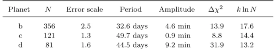
The individual transit times were then fitted with a linear function of epoch, and this function was subtracted from the timing data to isolate any timing residuals. A visual in-spection showed no obvious TTV signal in the residuals. We fitted these residuals with a sinusoidal model with three parameters: a TTV period, phase, and amplitude. To facilitate the exploration of the parameter space, we divided the range of periods into small intervals covering periods from 10 to 500 days, and for each period we optimized the other two pa-rameters. For the three planets, the best-fitting sinusoids gave unacceptably high χ2 values
relative to the number of degrees of freedom (2200, with 356 points for planet b, 198 with 121 points for planet c, and 200 with 81 points for planet d). The uncertainties on the individual transit times are likely underestimated due to correlated noise in the photomet-ric time series (due to some combination of stellar granulation, p-modes, and instrumental noise). We proceeded by enlarging the uncertainties by a scale factor (see Table 2) such that the minumum χ2 was equal to the number of degrees of freedom.
To search for a sinusoidal TTV signal for each of the planets, we used the Bayesian information criterion. The criterion requires that when k new parameters are introduced in a model, one needs to achieve a decrease in χ2 larger than k ln N, where N is the number of
data points, to justify the addition of the extra parameters. Table 2 shows that the additional
a bound companion having a density up to ≈ 1.5-times that of Kepler-65 (since it would still have shown detectable oscillations).
three parameters are only justified for Kepler-65d, and not for the other two planets. That planet d is singled out in this test is consistent with the hypothesis that all three planets orbit Kepler-65, as this planet has the longest orbital period and is closest to the largest and presumably most massive planet (Kepler-65c; see Section 3.2 and Table 3), factors which enhance the amplitude of the TTV signal. Its orbital period is 1.39 times that of Kepler-65c, making it near a 7:5 ratio. This has been observed in many other multiplanet systems (Fabrycky et al. 2012).
Even though the TTV signal of Kepler-65c did not satisfy the Bayesian information criterion for detection, the measured TTV period of the best-fitting sinusoid is close to the value expected from the formula of Agol et al. (2005), which for the c and d pair is 50 days (in agreement with the detected period). With more data one might be able to establish this signal more securely. Using the 0.9-min amplitude of this hypothetical signal as a reference, one would estimate a mass (or upper bound; see Lithwick et al. 2012) for Kepler-65d of approximately 10 ME.
We conclude that Kepler-65 is indeed transited by a system of three planets, based on the low false-alarm probability for each individual transit, the unlikely coincidence that would be required for a spurious system to produce the observed trend of transit durations versus orbital periods, the agreement between the photometric and asteroseismic estimates of the mean stellar density, and the detection of a physically reasonable TTV signal for at least one of the planets. However, as in many other cases, we acknowledge the fact that we cannot completely rule out the unlikely companion scenario, in which one or more of the planets orbits a fainter, bound companion having a higher density than Kepler-65.
Table 2. TTV signals of Kepler-65
Planet N Error scale Period Amplitude ∆χ2 k ln N
b 356 2.5 32.6 days 4.6 min 13.9 17.6 c 121 1.3 49.7 days 0.9 min 8.8 14.4 d 81 1.6 44.5 days 9.2 min 31.9 13.2
Note. — Summary of the search for sinusoidal TTV signals in the transit times of Kepler-65b, c and d. After correcting the timing error bars to account for correlated noise and low S/N, we find that only Kepler-65d has a significant detection.
3.2. Transit parameters for Kepler-50 and Kepler-65
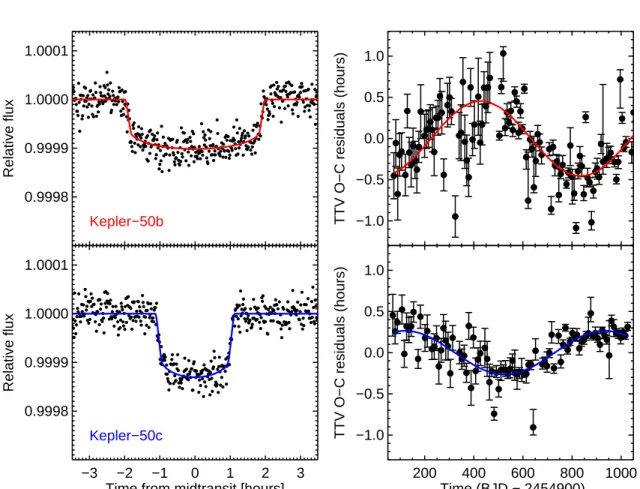
Transit timing variations are quite significant for Kepler-50. For this reason, care was needed in producing a phase-folded transit light curve for subsequent analysis. In addition to the three transit model parameters (R/a, b, (Rp/R)2) for each candidate and the two
limb-darkening coefficients, we modelled the interval between transits as a constant plus a sinusoidal function of time. We fitted this model to SC data (Q6 through Q11) for transits separated from each other by at least 6 hr and, using the best-fitting model, we folded the data and binned it to a cadence of 7.5 sec. This template was then used to obtain the transit timings with uncertainties as described in the previous section. The new TTV signal, including the long-cadence (LC) timings from the Kepler catalog, was then fitted to improve the sinusoidal component of the ephemeris, which in turn was used to properly fold the data. This iterative process converged when the sinusoidal component did not change significantly from one step to the next.
The final phase-folded light curves and the best-fitting models are shown in Fig. 4. The two planets have very similar orbital periods, with a period ratio close to 1.2. We see in the figure that the transits of the outer planet are much shorter in duration than those of the inner planet. This indicates that the transits of planet c have a high impact parameter. In this situation there is a risk of bias in the determination of the planet radius due to poorly constrained limb-darkening coefficients. To avoid this, we introduced Gaussian priors on each coefficient with values of 0.3 ± 0.1, based on the theoretical coefficients given by Claret & Bloemen (2011) for stars similar to Kepler-50. Since the orbits are so close to each other, we assumed circular orbits around the same star, essentially linking all of the R/a parameters for the two planets (see section 3.1.2). The resulting planet parameters are given in Table 3. The stellar density derived from this transit model has a large uncertainty due to the low S/N of the transits, but the final value 0.40+0.6−0.10g cm−3 is nevertheless compatible
with the much more precisely determined asteroseismic density of 0.441 ± 0.004 g cm−3 (see
Table 1 and Section 2).
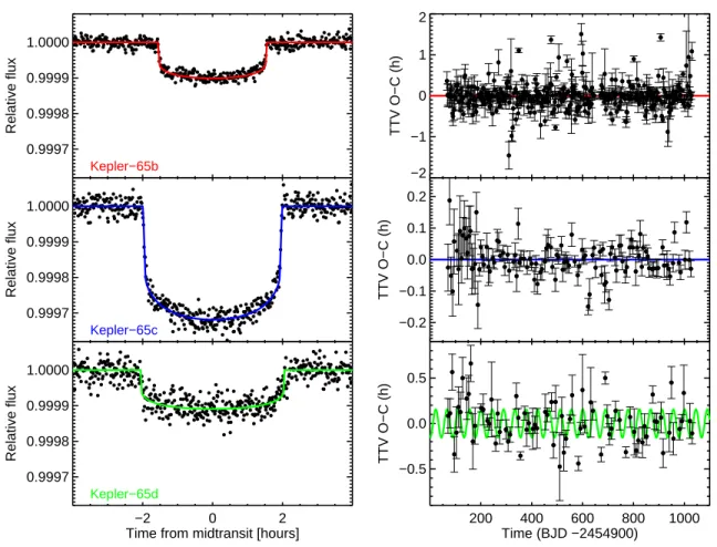
For Kepler-65 we used the analysis discussed in the previous section to construct the phase-folded light curves. Since no TTV signal was detected for planets b and c, a constant period was assumed in constructing the phase-folded light curves based on SC data. For planet d, the best-fitting sinusoidal TTV model was used to fold the transits. An individual analysis for each planet showed that the ingress duration of planet d was still larger than expected, by a factor of about two. This long ingress duration implies a large impact parameter, which again leads to large uncertainty and possible bias in the planetary radius. As for Kepler-50, we assumed the planets to be on circular orbits around the same star. The phase-folded light curves of all three transiting planets are shown in Fig. 5, along with the
0.9998 0.9999 1.0000 1.0001 Relative flux Kepler−50b −3 −2 −1 0 1 2 3
Time from midtransit [hours] 0.9998 0.9999 1.0000 1.0001 Relative flux Kepler−50c −1.0 −0.5 0.0 0.5 1.0
TTV O−C residuals (hours)
200 400 600 800 1000 Time (BJD − 2454900) −1.0 −0.5 0.0 0.5 1.0
TTV O−C residuals (hours)
Fig. 4.— Left-hand panels: the black dots show the binned SC (one-minute cadence) data for each of the Kepler-50 planets, and the lines show the best-fitting transit models. Right-hand panel: TTVs and uncertainties. The sinusoidal anti-correlated signals are plotted with thick lines.
0.9997 0.9998 0.9999 1.0000 Relative flux Kepler−65b 0.9997 0.9998 0.9999 1.0000 Relative flux Kepler−65c −2 0 2
Time from midtransit [hours] 0.9997 0.9998 0.9999 1.0000 Relative flux Kepler−65d −2 −1 0 1 2 TTV O−C (h) −0.2 −0.1 0.0 0.1 0.2 TTV O−C (h) 200 400 600 800 1000 Time (BJD −2454900) −0.5 0.0 0.5 TTV O−C (h)
best-fitting models.
Final values of the planet parameters are presented in Table 3. With the improved folded light curve for planet d, the stellar mean density (assuming circular orbits) is 0.61+0.02−0.10g cm−3,
which also agrees with the value obtained from asteroseismology. One could use the aster-oseismic density as a prior on our model, but this would not necessarily lead to greater accuracy because non-zero eccentricities cannot be ruled out for this system.
Finally, we note that in the transit analysis for both Kepler-50 and Kepler-65 we have assumed that the light from blended stars is negligible (i.e. a contamination factor of zero). This is well justified by the AO images (Adams et al. 2012). The contamination factors given in the Kepler Input Catalog are very low for both systems, and the uncertainties in the planetary radii are dominated by statistical uncertainties rather than the systematic effects of possible contamination.
3.3. Discussion of the coplanarity of the systems
In order to interpret the measured stellar obliquity in the context of the formation and evolution of the system, it is important to decide whether the planets are in coplanar orbits (Sanchis-Ojeda et al. 2012). The low S/N of the transit signals makes it difficult to use transit observables to constrain the mutual inclination, but the fact that we have found several planets transiting each star already tells us that these systems are likely to be coplanar (Lissauer et al. 2011). The probability that a planet on a randomly oriented circular orbit will transit a star is given by R/a. Using the values from Table 3 we may evaluate the probability for two extreme cases: (i) the planets have coplanar orbits; and (ii) their orbital orientations are uncorrelated. In the first case, if the most distant planet transits the star, the other planets in the system will also transit and so the probability of all planets transiting is equal to p1 = R/aq, where q refers to the most distant planet. If the planets’
orbits have independent random orientations, then the probability p2 that all planets will
transit is then equal to the product of the individual probabilities for each planet. Evaluating these probabilities p1 and p2 for Kepler-50, we find that p1/p2 = 10.5, i.e., the likelihood
for coplanar orbits is ten-times higher. For Kepler-65 the ratio is 55, favoring coplanar orbits even more strongly. Thus, both systems are likely to be nearly coplanar, although moderate mutual inclinations cannot be ruled out by this analysis. More definitive results might eventually be achieved through transit-timing studies or the detection of planet-planet eclipses (see, e.g., Hirano et al. 2012b).
4. Asteroseismic determination of stellar angle of inclination 4.1. Principles of the method
Asteroseismic estimation of the stellar angle of inclination, is, rests on our ability to
resolve and extract signatures of rotation in the non-radial modes from the oscillation spec-trum. Detailed descriptions of the principles of the asteroseimic method may be found in Gizon & Solanki (2003) and Ballot et al. (2006, 2008). Here, we summarize the key points. Rotation lifts the degeneracy in the oscillation frequencies νnl, so that the frequencies
of non-radial modes (l > 0) depend on the azimuthal order, m. For the fairly modest rates of rotation typical of solar-like oscillators we may ignore, to first order, the effects of the centrifugal distortion (e.g., see Reese et al. 2006; Ballot 2010). The 2l + 1 rotationally split frequencies may then be written:
νnlm≡ νnl+ δνnlm, (1) with δνnlm ≃ m 2π Z R 0 Z π 0 Knlm(r, θ)Ω(r, θ)r dr dθ. (2)
Here, Ω(r, θ) is the position-dependent internal angular velocity (in radius r, and co-latitude θ), and Knlm is a weighting kernel that reflects the sensitivity of the mode to the internal
rotation as a function of depth. For modest rates of differential rotation (in latitude and radius) and absolute rotation, the splittings δνnlmof the observable high-n, low-l p modes will
take very similar values, hence tending to the approximation of solid-body rotation (Ledoux 1951). Here, we found no evidence for significant mode-to-mode variation of the frequency splittings in the oscillation spectrum of either star. In what follows we therefore modelled all splittings as being equal, i.e., δνnlm = δνs. The above also neglects any contributions to
the splittings from near-surface magnetic fields, which give rise to frequency asymmetries of the observed splittings. The levels of activity in both stars – as revealed by signatures of rotational modulation of spots and active regions in the Kepler lightcurves – are notably lower than those displayed by the active Sun (see later, in Section 5). Since magnetic contributions to the solar low-l splittings are small in size and very hard to measure in Sun-as-a-star data of much higher S/N (e.g., see Gough & Thompson 1990; Chaplin 2011, and references therein), asymmetries here should not be a cause for concern for the analysis.
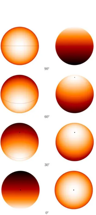
The determination of the inclination of the stellar rotation axis relies on the fact that the mode patterns of the non-radial modes are not spherically symmetric. The disk-integrated amplitudes of the m components in any given non-radial muliplet will therefore depend on the viewing angle. Fig. 6 shows a snapshot of the intensity perturbations of the m = 1
Fig. 6.— Intensity perturbations for l = 1 mode components, at a phase corresponding to extreme displacement of the oscillations. Plotted are patterns for m = 1 (left-hand column) and m = 0 (right-hand column) modes viewed at different angles, is = 90◦ (top row), 60◦
(second row), 30◦ (third row) and 0◦ (bottom row). The filled circles mark the pole of the
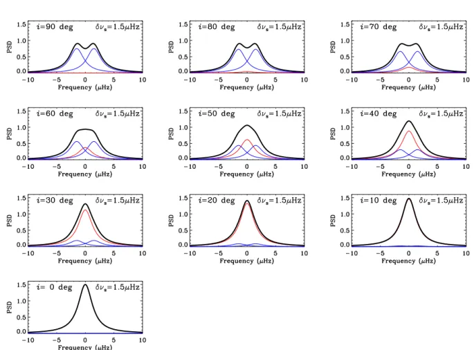
Fig. 7.— Theoretical profiles of an l = 1 mode observed at different stellar inclination angles, is. The m = ±1 components are plotted in blue, the m = 0 components in red, and the thick
black line shows the combined multiplet profile. The peak linewidth of each component is Γ = 3.0 µHz and the rotational frequency splitting is δνs = 1.5 µHz. Panels in the left-hand
(left-hand column) and m = 0 (right-hand column) components of an l = 1 mode viewed at different angles, is. The perturbations are shown at a phase corresponding to extreme
displacement of each oscillation mode. The filled circles mark the pole of the rotation axis and the lines show the stellar equator. Note that m = −1 perturbations are π out of phase with the m = 1 (and have not been plotted here). When the rotation axis lies in the plane of the sky (is = 90◦), the m = ±1 components presents their strongest observable amplitudes.
In contrast, the m = 0 component cannot be detected because the intensity perturbations in the northern and southern hemispheres cancel at all phases of the pulsation cycle, giving no disk-averaged signal. The situation is reversed at is = 0◦, when the rotation axis lies along
the line-of-sight and perturbations due to the m = ±1 components are no longer visible owing to geometric cancellation.
This dependence (measured in power) may be written explictly as: Elm(is) = (l − |m|)! (l + |m|)! h Pl|m|(cos is) i2 , (3)
where Pl|m|is the Legendre function, and the sum over Elm(is) is normalized to unity.
Measur-ing the relative power of the azimuthal components of different |m| in a non-radial multiplet therefore provides a direct estimate of the stellar angle of inclination, is, or more properly
|is| since symmetries inherent in Equation 3 mean we cannot discriminate between is and
−is, and π − is and π + is.
The above discussion rests on two assumptions. Firstly, that contributions to the ob-served stellar intensity across the visible stellar disk depend only on the angular distance from the disk centre. This is valid for photometric observations, where limb darkening con-trols the weighting. Secondly, that there is equipartition of energy between the different m components3. This should be valid except in very rapid rotators where rotation can
af-fect convection, which excites and damps the modes. The predicted power asymmetries (Belkacem et al. 2009) of our stars are of the order of 1 %, which are negligible for our analysis.
Fig. 7 shows the appearance in the frequency-power spectrum of an idealized l = 1 multiplet as a function of the angle is (see also Gizon & Solanki 2003). Panels in the
left-hand column correspond to the cases shown in Fig. 6. The l = 1 modes are approximately three times more prominent in the frequency-power spectrum than the l = 2 modes (see,
3
While the case for stochastically excited and intrinsically damped solar-like oscillations leads to energy equipartition, for observations made over a sufficient number of lifetimes, this is not so for classical “heat-engine” pulsators (e.g., the γ Doradus, δ Scuti and white-dwarf classes).
e.g., Ballot et al. 2011b). Hence, it is these modes that largely constrain our ability to infer is.
The individual components in Fig. 7, which are plotted in blue (m = ±1) and red (m = 0), were modelled as Lorentzian functions, the underlying function used to describe the damped p modes. The width Γ of each Lorentzian – which is proportional to the mode damping rate – is 3.0 µHz, which corresponds approximately to the linewidths observed in the most prominent l = 1 modes of Kepler-50 and Kepler-65. The splitting is δνs = 1.5 µHz,
which corresponds to a rotation period of 7.7 d, and so matches approximately what we observe for the two stars. The thick black lines show the combined multiplet profiles.
Given sufficient resolution in frequency and good S/N in the modes, it is the ratio δνs/Γ of intrinsic stellar properties that determines whether it is possible to resolve the
components, and hence to infer the true underlying Elm(is) and hence the value of is. As
noted previously, at angles close to 90◦ the m = 0 component has insignificant visibility and
the overall appearance is dominated by the |m| = 1 components (the converse being true at angles close to 0◦). Uncertainties in the inferred angle will be largest when the i
s matches
these extreme cases, all other factors being equal (Ballot et al. 2008). This is because there are then only modest variations in the overall appearance of the mode multiplet with changing is.
4.2. Estimation of stellar inclination angles
Extracting the required information from the rotationally split components proceeds via a careful fitting of the modes in the observed frequency-power spectrum, sometimes referred to as peak-bagging (see Appourchaux et al. 2012, and references therein, for further results on Kepler targets).
Frequency splittings δνs due to rotation are clearly visible in the oscillation spectra of
both stars. Fig. 8 shows two prominent l = 1 modes in each star. The light grey lines plot the observed spectra after applying a light amount of smoothing. The thick dark grey lines follow the spectra after they have been smoothed with a filter of width 1.5 µHz, which provides an approximate representation of the underlying (noise-free) profiles. Even without a detailed analysis it is apparent that the observed modes bear a striking resemblance to the high-inclination cases in Fig. 7. The dark-blue lines follow the best-fitting Lorentzian models, which we describe below.
The observed frequency-power spectrum P(ν) of each star was modelled as
Fig. 8.— Prominent l = 1 modes in the frequency power spectra of Kepler-50 (top panels) and Kepler-65 (bottom panels). Light grey lines: observed spectra after applying light smoothing. Thick dark grey lines: observed spectra after applying a heavier smoothing of width 1.5 µHz. Dark-blue lines: best-fitting models from MCMC analysis.
where O(ν) describes the oscillations and B(ν) contains background terms due to granu-lation, activity and photon shot noise. The oscillations O(ν) were modelled as a series of Lorentzian profiles describing the stochastically excited and intrinsically damped modes. We adopted a global description, in which we modelled simultaneously all the observable modes instead of modelling and analyzing the spectrum one order at a time. This approach im-proves the accuracy of the modelling because it takes proper account of the power from the slowly decaying Lorentzian peaks that bleeds in frequency between the neighbouring modes. The modelled oscillations spectrum was thus described by:
O(ν) =X n′,l l X m=−l Elm(is)Hn′l 1 + 4/Γ2 n′(ν − νn′l− mδνs)2 , (5)
The inner sum in the above runs over the m components of each rotationally split multiplet; while the outer sum runs over all observed modes, in radial order n, and degree l. Note that the dummy variable n′, which tags the radial order, takes values n′ = n for l = 0 and l = 1
modes, and n′ = n − 1 for l = 2 modes (which lie adjacent in frequency to l = 0 modes of
n′ = n). The angle i
s and single splitting parameter δνs are two of the parameters to be
optimized, along with the frequencies νnlused to estimate the fundamental stellar properties
(Section 2).
The parameters Hnland Γn describe the height (maximum power spectral density) and
linewidth of each mode. We fit a single linewidth parameter to each order. The relative heights of the components in each non-radial multiplet are controlled by is through the
function Elm(is) (Equation 3). The heights are constrained by the relation Hn′l = Hn′0V2
l ,
where the parameter V2
l describes the visibilities of modes of different l, relative to l = 0. The
visibilities are given by integrating the spherical harmonic functions over the visible disk with suitable allowance made for limb darkening and the spectral bandpass of the observations (Ballot et al. 2011b). We adopted fixed values of V2
0 = 1.0, V12 = 1.5 and V22 = 0.5 in our
analysis.
The background was modelled as the sum of three components: a flat photon shot-noise component, W , and two frequency-dependent components to describe contributions from granulation and activity. For the latter components, we used functions based on the Lorentzian-like forms proposed by Harvey (1985), which provide a good description of the observed backgrounds in solar-type stars (e.g., see Metcalfe et al. 2012). The composite background was then described by:
B(ν) = W + 2 X k=1 4σ2 kτk 1 + (2πτkν)2+ (2πτkν)4 , (6)
component. The granulation and activity components each have two free parameters to be optimized: σk is related to the RMS amplitude of the signal in the time domain, while τk
is the characteristic timescale of the decaying autocorrelation function. For granulation, σ and τ are smaller than the corresponding activity parameters.
We adopted two different approaches to the fitting, and hence to estimation of is. In
the first approach the parameters of the model in Equation 4 were optimized using a MCMC approach, as described by Handberg & Campante (2011). We adopted a flat prior for is
between 0◦ and 90◦. In order to avoid the rejection of sample jumps close to the boundaries
– i.e., those that would jump beyond the range set by the prior – in practice we selected from samples in the range −90◦ to 180◦ and modified accepted jumps that went beyond the
allowed range by reflecting about the is = 0◦ and 90◦ boundaries. A flat prior was imposed
on δνs, running between zero and 2.5 µHz for Kepler-50, and zero and 5 µHz for Kepler-65.
Besides making it possible to incorporate relevant prior information through Bayes’ theorem, the MCMC approach also gave the marginal probability density function (PDF) of each of the model parameters (e.g., see discussion in Appourchaux 2011). In order to provide a cross-check we also used Maximum Likelihood Estimation (MLE) to fit the spectrum (e.g. see Duvall & Harvey 1986; Toutain & Appourchaux 1994), using the so-called pseudo-global fitting described by Fletcher et al. (2009). Rather than fit the is directly with MLE, we
instead performed a series of MLE fits with the angle fixed at different values, the aim being to sample the maximized likelihood of the best-fitting model as a function of the chosen is.
Even though is is independent of the splitting parameter δνs, the measured values are often
highly correlated (e.g., see Ballot et al. 2006, 2008). In order to constrain the two individual parameters, or their combination the so-called reduced splitting (i.e., δνs sin is), it is desirable
to have access to the corresponding maximized likelihood in two-dimensional parameter space. We therefore performed fits with both is and δνs taking values on a dense grid. This
yielded a two-dimensional grid of maximized likelihoods, making possible inference on the inclinaton and splitting from construction of confidence intervals based on the likelihood surface. The MLE approach had the advantage of being more computationally efficient than the MCMC analysis. However, given that the input values for the inclination and splitting are fixed prior to the fitting, one cannot extract a bona fide posterior probability distribution. The MCMC and MLE approaches returned results in excellent agreement. Here, we present those given by the MCMC approach.
Table 4 lists the final MCMC estimates of the inclinations and splittings, together with their corresponding 1σ credible regions. The estimated is of both stars are consistent
with 90◦, to within the uncertainties. We note that the final values for the splittings were
given by the median of each posterior distribution, while for the angles we opted to use the mode of each distribution. The rationale behind this decision was twofold. Firstly, the
PDF of the inclination is truncated at is = 90◦ and the median is thus not a representative
statistic of the distribution. Secondly, in each case the model of the oscillations spectrum built by using the mode for the inclination, together with the median for all the remaining parameters (including the splitting) has a higher posterior likelihood than the models made using exclusively either the median or the mode for all parameters.
As noted above, the thick black lines in Fig. 8 show best-fitting models from the MCMC analysis across frequency ranges occupied by two l = 1 modes in each star. Figs. 9 and 10 show the correlation maps in the angle and splitting, as well as the PDFs obtained after marginalization. Binwidths for the PDFs were fixed by following the procedure given in Scott (1979) [see also Handberg & Campante 2011].
5. Comparison with measures of surface rotation
We have compared the asteroseismic results from Section 4.2 with two independent estimates of the surface rotation: one extracted from signatures of rotational modulation in the Kepler lightcurves, and another extracted from spectroscopic data on both stars.
If a star has spots on its surface then rotation will carry the spots in and out of view, inducing quasi-periodic flux variations. Such variations have been detected for many stars, and it is not unusual to see activity in stars as hot as our host stars (Basri et al. 2011). The rotation period of Kepler-50 has already been detected in Kepler data (Hirano et al. 2012a) and Kepler-65 also shows clear signs of rotational modulation in its lightcurve.
The raw Kepler data are known to suffer from systematic trends that appear to be shared by most of the stars on a given CCD detector module. The absolute effect of these trends on the measured stellar fluxes is much larger than the activity levels for both stars, so we needed to choose an appropriate detrending algorithm that would suppress the unwanted systematics without removing the astrophysical signal. One such algorithm available to us is PDC-MAP (Stumpe et al. 2012, Smith et al. 2012), which was developed by the Kepler team. Principal component analysis is used to extract a basis of co-trending vectors that capture the systematic trends in each module. Each stellar flux datum may be decomposed into a linear combination of the astrophysical variability and the co-trending vectors. One could perform a least-squares fit to extract those coefficients but PDC-MAP goes one step further. During a first pass on the data it applies a least-squares approach to obtain the coefficients for all stars that fall on a given detector module. The distributions are then used as priors in a Bayesian sense, thereby mitigating possible over-correction of the time series for any individual star. PDC-MAP appears to do a reasonable job of eliminating the systematic
Table 3. Transit parameters
Parameter Kepler-50b Kepler-50c Kepler-65b Kepler-65c Kepler-65d (Rp/R)2 [ppm] 99+5−11 159+10−11 85.0+1.6−1.1 282 +5 −2 98 +2 −2 Impact parameter b 0.74+0.07 −0.36 0.94+0.02−0.06 0.16+0.20−0.11 0.42+0.10−0.02 0.53+0.07−0.02 R/a 0.095+0.015 −0.025 0.084+0.013−0.022 0.188+0.011−0.002 0.097+0.006−0.001 0.078+0.005−0.001 LD coefficient u1 0.28+0.08−0.08 – 0.25+0.07−0.08 – – LD coefficient u2 0.29+0.08−0.07 – 0.37+0.11−0.10 – –
Transit duration T1.5−3.5[hours] 3.80+0.05−0.03 2.06 +0.03 −0.03 3.077 +0.07 −0.007 3.928 +0.008 −0.007 4.10 +0.02 −0.03
Orbital period [days] 7.81254(10) 9.37647(4) 2.154910(5) 5.859944(3) 8.13123(2) Time of transit [BJD-2454900] 74.376(7) 69.958(3) 66.4990(13) 65.0391(3) 70.9905(16) Planet radius [RE] 1.71+0.05−0.10 2.17+0.07−0.08 1.42+0.03−0.03 2.58+0.06−0.06 1.52+0.04−0.04
Semi-major axis [AU] 0.077+0.012−0.020 0.087+0.014−0.023 0.035+0.002−0.001 0.068+0.004−0.002 0.084+0.006−0.002
Note. — Summary of planetary parameters. The first five parameters were estimated from the folded light curve analysis, and the durations were obtained from those parameters. Uncertainties come from an MCMC analysis. Orbital periods and times of transit come from a fit to the transit times, with a sinusoidal component in the case of Kepler-50 and only a linear term for Kepler-65. Estimation of planetary radii and semi-major axes also made use of the stellar radii from the asteroseismic analysis.
Table 4. Estimated stellar inclinations and rotational splittings
Star is sin i δνs≡ Ω/2π
(degrees) (µHz)
Kepler-50 82+8−7 0.99+0.01−0.02 1.51+0.09−0.08
Kepler-65 81+9
Fig. 9.— Asteroseismic results on Kepler-50. Lower left-hand panel: Correlation map in angle of inclination is and rotational frequency splitting δνs (highest likelihoods rendered in
red); Top and right-hand panels: PDFs obtained after marginalization. Note that the PDFs are normalized so that the integral under each curve is unity. Bold crosses mark the final parameter estimates given in Table 4.
trends in almost every quarter of data, but does fail on a few occasions. From the available long-cadence (LC) data (Jenkins et al. 2010) collected through Q11, we discarded the Q3 and Q11 data for Kepler-50, and the Q7 and Q8 data for Kepler-65. Outliers were also removed by performing 3σ clipping using a 10-hour-long moving-median filter. The remaining data were quite adequate to estimate robust rotation periods. The left-hand panels of Fig. 11 show three-month segments of the data, in which intrinsic stellar variability on time scales of days is evident. This variation is smaller than that displayed by the active Sun (e.g., see Basri et al. 2010, 2011), for which the semi-amplitude of the variability reaches levels close to 1 part in 103.
To extract estimates of the surface rotation periods we followed the analysis described by Hirano et al. (2012a). We first calculated the Lomb-Scargle periodogram of each set of processed data, which are plotted in the right-hand panels of Fig. 11. Both stars show significant peaks around 8 days due to rotational modulation of spots. We checked that our results did not depend on the detrending, as follows. Firstly, we used the simple least-squares fit to the co-trending vectors described above. Secondly, we applied a 20-day median smoothing filter to divide the raw data. Both approaches led to periodograms in good agreement with our main results.
Both stars show several significant, closely spaced peaks in their periodograms. The spread in period of the peaks will have contributions from the finite spot lifetimes and might also suggest the presence of surface differential rotation. Fig. 11 also shows periodograms obtained from particular subsets of the data, which suggest that the rotation periods might be evolving with time. Again, this might be associated with stochastic variability due to the spot lifetimes, or it could have a contribution due to changes in the spot latitudes. These signatures are not unexpected for such hot stars (Collier Cameron 2007) but the low S/N of the stellar variability in the lightcurves makes it hard to test the results in greater detail. It is worth adding that we also checked that the spread of significant periods was not an artifact of the observational window function. We sampled commensurate sine waves of period 8 d at the same time stamps as the real, cleaned PDC-MAP lightcurves, and found that the resulting periodograms displayed a much smaller width of significant periods than the real data (of order 0.2 to 0.4 d).
As in Hirano et al. (2012a), for each star the continuous range of periods containing all peaks with more than half the power of the highest peak was taken as the uncertainty on the surface rotation period, with the center of the range adopted as the quoted period, Prot.
The rotation periods obtained in this way were 8.4 ±1.0 days for Kepler-50 and 8.4 ±0.3 days for Kepler-65. The rotational frequency splittings δνs given by the asteroseismic analysis are
Kepler-65. The close agreement between the surface and internal rotation rates is consistent with the expectation that the frequency splittings of p modes observed in main-sequence stars are largely determined by the rotation profile in the stellar envelope (as in the case of the Sun).
We can also compare our results with v sin is estimates extracted from the spectroscopic
data (see Section 2). For Kepler-50 the spectroscopic analyses gave 8.6 ± 0.8 km s−1 (SME)
and 10.3±0.5 km s−1(SPC), while for Kepler-65 they gave 9.8±0.8 km s−1 (SME) and 11.9±
0.5 km s−1 (SPC). To compare with the asteroseismic results, we converted the estimated
rotational frequency splittings to projected rotational velocities using
v sin is≡ 2πR δνssin is, (7)
with the stellar radii R given by the asteroseismic analysis discussed in Section 2. These conversions gave equivalent asteroseismically determined projected velocities of 8.0+1.2−1.0km s−1
for Kepler-50 and 10.4 ± 0.6 km s−1 for Kepler-65. Again, we find agreement between the
asteroseismic and surface estimates. We note that the SPC v sin is values are higher than
the SME values by about 20 %, in agreement with the findings by Torres et al. (2012). Finally, we may combine the spot modulation and v sin is results to provide independent
estimates of is, via
sin is = Prot(v sin is)/(2πR). (8)
When we used the SME results for v sin is we found that sines of the angles were constrained
at the 1σ level to lie above 0.89 for Kepler-50 and 0.90 for Kepler-65, again implying that both stars have their rotation axes nearly perpendicular to the line of sight. When the SPC v sin is were used we obtained sin is > 1.0 for both systems suggesting that (at least for
these systems) the SPC results are overestimated.
6. Discussion
Our central result is that the host stars of the Kepler- 50 and Kepler-65 planetary sys-tems have their rotation axes nearly perpendicular to the line of sight, with sin isconstrained
at the 1σ level to lie above 0.97 and 0.91, respectively. Expressed in terms of angles, we have |90◦ − i
s| < 15◦ for Kepler-50 and < 25◦ for Kepler-65. The orbital inclinations of the
planets in each system are also near 90◦, with a deviation of only ≈ 5◦ for the planets of
Kepler-50 and ≈ 2◦ for the planets of Kepler-65. Therefore our observations are consistent
with small differences in the stellar and orbital inclination angles, and low stellar obliquities. A limitation of the results is that it is possible for the obliquity to be large but for the difference in inclination angles to be small. Spherical geometry dictates that the 3D obliquity