Beam-induced and cosmic-ray backgrounds observed in the ATLAS detector during the LHC 2012 proton-proton running period

EUROPEAN ORGANISATION FOR NUCLEAR RESEARCH (CERN)

Submitted to: JINST CERN-EP-2016-029

21st August 2018

Beam-induced and cosmic-ray backgrounds observed in the

ATLAS detector during the LHC 2012 proton-proton running

period

The ATLAS Collaboration

Abstract

This paper discusses various observations on beam-induced and cosmic-ray backgrounds in the ATLAS detector during the LHC 2012 proton-proton run. Building on published results based on 2011 data, the correlations between background and residual pressure of the beam vacuum are revisited. Ghost charge evolution over 2012 and its role for backgrounds are evaluated. New methods to monitor ghost charge with beam-gas rates are presented and observations of LHC abort gap population by ghost charge are discussed in detail. Fake jets from colliding bunches and from ghost charge are analysed with improved methods, showing that ghost charge in individual radio-frequency buckets of the LHC can be resolved. Some results of two short periods of dedicated cosmic-ray background data-taking are shown; in particular cosmic-ray muon induced fake jet rates are compared to Monte Carlo simulations and to the fake jet rates from beam background. A thorough analysis of a particular LHC fill, where abnormally high background was observed, is presented. Correlations between backgrounds and beam intensity losses in special fills with very high β∗are studied.

Keywords: Beam-line instrumentation, Data analysis, Performance of High-energy Physics Detectors.

c

2018 CERN for the benefit of the ATLAS Collaboration.

Reproduction of this article or parts of it is allowed as specified in the CC-BY-4.0 license.

Contents

1 Introduction 3

2 The LHC and the ATLAS detector 4

2.1 The LHC collider 4

2.2 The ATLAS detector 7

3 Non-collision backgrounds 8

4 Background monitoring methods 9

4.1 Background monitoring with the BCM 9

4.2 Using LUCID luminosity data in background analysis 11

4.3 Using calorimeter jets in background analysis 11

4.4 Pixel background tagger 12

5 Data-taking Conditions 13 6 Afterglow 14 7 Background monitoring 18 7.1 Beam-gas events 18 7.2 Ghost collisions 19 8 Fake jets 27

8.1 Fake jets in unpaired bunches 28

8.2 Non-collision backgrounds in colliding bunches 31

8.3 Fake jets in cosmic-ray events 34

9 BIB from ghost charge 37

9.1 BCM background from ghost charge 37

9.2 Fake jets from ghost bunches 40

9.3 Ghost bunches in the abort gap 42

10 Backgrounds in special fills 46

10.1 High background fill 46

10.2 Background in high-β∗fills 49

10.3 Backgrounds during 25 ns operation 56

11 Conclusions 56

1. Introduction

In 2012 the Large Hadron Collider (LHC) increased its beam energy to 4 TeV and raised beam intensities with respect to 2011. Bunch intensities up to 1.6×1011protons were routinely reached.

The high-luminosity experiments at the LHC are designed to cope with intense background from pp collision debris, compared to which the usual levels of beam-induced backgrounds (BIB) are negligible. When beam intensities and energies increase, the risk for adverse beam conditions, that could compromise the performance of inner detectors, grows. In order to rapidly recognise and mitigate such conditions, a thorough understanding of background sources and observables is necessary. The main purpose of this paper is to contribute to this knowledge.

The experience accumulated during the 2011 operation, in measuring and monitoring beam backgrounds [1], allowed optimisation of the beam structure and analysis procedures to reach better sensitivity for background observables. In this paper, a summary of the main observations on BIB and cosmic-ray backgrounds (CRB), as well as ghost collision rates, in the ATLAS detector is presented. The topics cover a variety of background types in different experimental conditions encountered in 2012.

The operational conditions of the LHC, relevant for this analysis, are first explained, followed by a short discussion of the background detection and triggering methods. Subsequent sections are devoted to de-tailed analyses, starting with re-establishing the correlation between vacuum quality and BIB in the AT-LAS inner detector region, refining the analysis already performed on 2011 data.

Improved methods to monitor ghost collisions, i.e. protons (ghost charge) in nominally empty radio-frequency (RF) buckets of the LHC colliding with nominal intensity bunches in the other beam (unpaired bunches), are introduced and used to separate beam backgrounds in unpaired bunches into collision, beam-gas and random noise components. Implications for correcting luminosity measurements using unpaired bunch backgrounds are discussed.

The most significant non-collision background for physics searches comes from fake jets created by radiative energy losses of BIB or CRB muons in the calorimeters. Although the rate of such fake jets is low they still can form a non-negligible background in searches for rare physics processes. The sources, rates and characteristics of fake jets are discussed in detail and it is shown that in normal physics conditions the dominant fake jet background comes from BIB, although the fraction of fake jets from CRB increases towards higher apparent pT.

With the new, more sensitive, analysis methods it is possible to detect and quantify the BIB from ghost charge, despite the very low rate. Several unexpected observations are discussed, the most significant being the dominant role of the LHC momentum cleaning as a source of BIB. In particular, it is shown that BIB from ghost charge in the LHC abort gap can be detected by ATLAS. The effects of the LHC abort gap cleaning mechanism on these backgrounds are evaluated and it is shown that the abort gap is repopulated within about one minute when the cleaning is switched off. Although the levels of BIB from ghost charge are tiny, they can be observed clearly also as fake jets, which are significantly out of time. In searches for rare long-lived particles, such special backgrounds need to be rigorously removed. The 2012 operation included two fills with very special characteristics. The first was a normal fill, but following a magnet quench close to ATLAS. This quench caused local outgassing and resulted in very high backgrounds at the start of the fill. A detailed analysis of these backgrounds provides insights into the conditioning process of the beam pipe surface.

The other fill of interest used special optics for forward-physics experiments. The fill had very low beam intensity and luminosity, but large loss spikes due to repeated tightening of the betatronic beam cleaning. These conditions allow detail studies of correlations between losses at the LHC collimators and backgrounds seen in ATLAS. Although the optics was very different from high-luminosity operation, the methods developed and results obtained motivate similar tests during LHC Run-2 with normal optics but special low-intensity beams.

At the very end of 2012, three fills were dedicated to studies of operation with 25 ns bunch spacing, which is the baseline condition for LHC Run-2. Although only one of these fills was of sufficient length and intensity for backgrounds analysis, the observations will provide a useful point of comparison between the end of LHC Run-1 and the start-up after the long shutdown.

2. The LHC and the ATLAS detector

The LHC accelerator and the ATLAS detector are described in references [2] and [3], respectively. Only a concise summary is given here, focusing on aspects relevant for the 2012 background analysis.

2.1. The LHC collider

The features of the LHC, relevant to background, have been described in reference [1] and remained largely the same for the 2012 operation.

The RF of the LHC is 400.79 MHz and the revolution time 88.9244 µs, which means there are 35640 RF buckets that can accommodate particles. Nominally, only every tenth bucket can be filled and groups of ten buckets are identified with Bunch Crossing IDentifiers (BCID), which take values in the range 1–3564.

In order to be able to safely eject the full-energy LHC beam, an abort gap of slightly more than 3 µs is left in the bunch pattern to fully accommodate the rise-time of the beam extraction magnet. For the safety of the LHC it is imperative that the amount of ghost charge in the abort gap, especially its early part, does not become too large.

The LHC layout, shown in figure1, comprises eight arcs, which are joined by Long Straight Sections (LSS) of slightly more than 250 m half-length. Each LSS houses an Interaction Region (IR) in its middle, the ATLAS detector being located in IR1. The LHC beam cleaning equipment is situated in IR3 (mo-mentum cleaning) and IR7 (betatron cleaning), i.e. two octants away from ATLAS for 2 and beam-1, respectively. The role of the beam cleaning is to intercept the primary and secondary beam halo, but some protons escape, forming a tertiary halo.1 In order to intercept this component and to provide local protection against accidental beam losses, tertiary collimators (TCT2) are placed about 150 m from the experiments on the incoming beams. The aperture settings of collimators, with respect to the nominal normalised emittance of 3.5 µm, are listed in table1. It can be seen that the momentum cleaning collim-ators in IR3 are much more open than those of the betatron cleaning in IR7. Since most of the cleaning

1_{The definition of the halo hierarchy is related to table1. The primary collimators intercept the primary beam halo, but some}

protons scatter out and form the secondary halo which is intercepted by the secondary collimators, which scatter out some tertiary halo that ends up on the tertiary collimators.

Momentum Cleaning ALICE Low ɴ (Ions) Injection RF CMS Low ɴ (protons) Dump Betatron Cleaning LHCb B-Physics Injection ATLAS

C

A

Figure 1: The general layout of the LHC [4]. The dispersion suppressors (DSL and DSR) are sections between the straight section and the regular arc. In this paper they are considered to be part of the arc, for simplicity. LSS denotes the Long Straight Section – roughly 500 m long parts of the ring without net bending. All insertions (experiments, cleaning, dump, RF) are located in the middle of these sections. Beams are injected through transfer lines TI2 and TI8. The ATLAS convention of labelling sides by ‘A’ and ‘C’ is indicated.

β∗ _{TCP in IR7 (in IR3) TCS in IR7 (in IR3) TCT in IR1,5 (in IR 2,8)}

0.6 m 4.3 (12) 6.3 (15.6) 9.0 (12)

1000 m 2.0†(5.9†) 6.3 (15.6) 17 (26)

Table 1: Apertures of primary (TCP), secondary (TCS) and tertiary (TCT) collimators in units of nominal betatronic σ, corresponding to a normalised emittance of 3.5 µm [5]. Settings for normal high-luminosity optics (β∗= 0.6 m) and the special high-β∗fill (β∗ = 1000 m), discussed in section10.2, are given. †For the 1000 m optics, the given TCP settings varied and the values listed correspond to the tightest settings.

takes place in IR7, it has much more efficient absorbers than IR3 so that per intercepted proton there is more leakage of cleaning debris from the latter.

The inner triplet of quadrupoles, providing the final focus, operates at 1.9 K and extends from z = 23 m to z = 54 m. It is equipped with a perforated beam-screen, operated at 20 K, in order to protect the

su-perconducting coils from synchrotron radiation, electron cloud effects and resistive heating by the image currents of the passing beam. The perforation allows for residual gas to condense on the cold bore of the coils. This cryo-pumping effect is responsible for the very low pressure reached in the cold sections of the LHC [6].

The residual pressure close to the experiment is monitored by several vacuum gauges of Penning and ionisation types. The 2011 background analysis revealed that the BIB seen in ATLAS at small radius is correlated with the pressure measured at 22 m. Further gauges are at 58 m (on accelerator side of inner triplet), 150 m (close to the TCT) and ∼250 m (at exit of the arc) from the IP. All of these were considered in the analysis but finally only the 22 m and 58 m readings were found to show a correlation with the observed backgrounds. The gauge at 58 m is located in a short warm section without Non-Evaporative Getter coating [7]. Electron-cloud formation was discovered to be a problem in this region and already in 2011 solenoids were placed around the beam-pipe in order to suppress electron multipacting. The solenoids were found to be efficient and remained operational throughout 2012.

The inner triplet quadrupole absorber (TAS) is another machine element of importance for background formation. It is a 1.8 m long copper block located at z= 19 m from the interaction point (IP) with a 17 mm radius aperture for the beam. While the TAS provides a shielding effect against beam backgrounds, high-energy particles impinging on it can initiate showers that are sufficiently penetrating to partially leak through.

A few thousand beam loss monitors (BLM) are distributed all around the LHC ring in order to monitor beam losses and to initiate a protective beam dump in case of a severe anomaly. The time resolution of a BLM is limited by its electronics to about 40 µs, so it cannot be used to determine loss rates of individual bunches. Since the BLMs are located around very different machine elements, with different internal shielding, their response with respect to one lost proton is not uniform. Thus, without detailed response simulations, the BLMs cannot be used to compare the losses in two different locations. They serve mainly to give information about the time development of losses on a given accelerator element. The loss-rates on the TCT would be most interesting for background studies. Unfortunately, in this location, the BLMs are subject to intense debris from the collisions, so during physics operation they have no sensitivity to halo losses.

Another beam monitoring system is the Longitudinal Density Monitor (LDM), which is used to measure the population in each RF bucket by synchrotron light emission [8]. The system has sufficiently good time resolution and charge sensitivity to detect ghost charge in individual RF buckets with an intensity several orders of magnitude below the nominal bunch intensity of ∼ 1011protons/bunch. In 2012 the system was operational only in some LHC fills and elaborate calibration and background subtraction had to be developed in order to extract the signal.

The beam intensity is measured by two devices of which only one, the fast beam current transformer (FBCT), provides intensity information bunch by bunch. Where appropriate, the intensity values provided by the FBCT have been used to normalise backgrounds.

Normal data-taking happens in the STABLE BEAMS mode. This is preceded by phases called FLAT TOP, when beams have reached full energy, SQUEEZE, when the optics at the interaction points is changed to provide the low β∗focusing for physics3 and ADJUST, during which the beams are brought

3_{The β-function determines the variation of the beam envelope around the ring and depends on the focusing properties of the}

into collision. Together FLAT-TOP and SQUEEZE last typically 20 minutes. During this time the beams remain separated, which provides particularly clean conditions for background monitoring.

2.2. The ATLAS detector

ATLAS is a general purpose detector at the LHC with almost 4π coverage. It is optimised to study proton-proton collisions at the highest possible energies, but has capabilities also for heavy-ion and very forward physics. The ATLAS inner detector is housed inside a solenoid which produces a 2 T axial field. It is surrounded by calorimeters and a muon spectrometer based on a toroidal magnet configuration. The calorimeters extend up to a pseudorapidity |η| = 4.9, where η = − ln tan(θ/2), with θ being the polar angle with respect to the nominal LHC beam-line in the beam-2 direction. Charged particle tracks are measured by the inner detector in the range |η| < 2.5. In the right-handed ATLAS coordinate system, with its origin at the nominal IP, the azimuthal angle φ is measured with respect to the x-axis, which points towards the centre of the LHC ring. As shown in figure1, side A of ATLAS is defined as the side of the incoming, clockwise, LHC beam-1 while the side of the incoming beam-2 is labelled C. The coding of LHC machine elements uses letters L (left of IR, when viewed from ring centre) for ATLAS side A and, correspondingly, R for side C. The z-axis in the ATLAS coordinate system points from C to A, i.e. along the beam-2 direction. The most relevant ATLAS subdetectors for the analyses presented in this paper are the Beam Conditions Monitor (BCM) [10], LUCID, the calorimeters, and the Pixel detector.

The BCM detector consists of 4 diamond modules (8 × 8 mm2 active area) on each side of the IP at a z-distance of 1.84 m from the IP and a mean radius of r = 5.5 cm from the beam-line, corresponding to |η| = 4.2. The modules on each side are arranged in a cross, i.e. two in the vertical plane and two in the horizontal plane. The individual modules will be referred to as Ax-, Cy+, etc. where the first letter refers to the side according to ATLAS convention, the second letter to the azimuth and the sign is according to the ATLAS coordinate system.

The LUCID detector was introduced as a dedicated luminosity monitor. It consists of 16 Cherenkov tubes per side, each connected to its own photomultiplier (PMT), situated in the forward region at a distance z = 18.3 m from the IP, giving a pseudorapidity coverage of 5.6 < |η| < 6.0. In 2012 LUCID was operated without gas in the tubes, most of the time. In this configuration, only the Cherenkov light from the quartz-window of a PMT was used for particle detection.

The Pixel detector consists of three barrel layers at mean radii of 50.5 mm, 88.5 mm and 122.5 mm. All layers have a half-length of 400 mm, giving an |η|-coverage out to 1.9 and 2.7 for the outermost and innermost layers, respectively. In each layer the modules are slightly tilted with respect to the tangent. The pixel size in the barrel modules is rφ × z = 50 × 400 µm. The full coverage, with three points per track, is extended to |η|= 2.5 by three endcap pixel disks.

A high-granularity liquid-argon (LAr) electromagnetic calorimeter with lead as absorber material covers the pseudorapidity range |η| < 1.5 in the barrel region. The half-length of the LAr barrel is 3.2 m and it extends from r = 1.5 m to r = 2 m. The hadronic calorimetry in the region |η| < 1.7 is provided by a scintillator-tile calorimeter (TileCal), extending from r = 2.3 m to r = 4.3 m with a half-length of 8.4 m. Hadronic endcap calorimeters (HEC) based on LAr technology cover the range 1.5 < |η| < 3.2. The absorber materials are iron and copper, respectively. The calorimetry coverage is extended by the Forward Calorimeter up to |η|= 4.9. All calorimeters provide nanosecond timing resolution.

3. Non-collision backgrounds

The non-collision backgrounds (NCB) are defined to include CRB and BIB. The main sources of the latter are [1,11]:

• Inelastic beam-gas events in the LSS or the adjacent arc. Simulations indicate that contributions from up to about 500 m away from the IP can be seen [12].

• Beam losses on limiting apertures. The contributions to the experiments come predominantly from losses on the TCTs, which in the normal optics are the smallest apertures in the vicinity of ATLAS. • Elastic beam-gas scattering around the ring. According to simulations [11,12], the scattered pro-tons are intercepted by the beam cleaning insertions or the TCTs. In the latter case their effect adds to the halo losses on the TCTs.

Beam-gas events, within about ±50 m from the IP, can spray secondary particles on the ATLAS inner detectors, but it is unlikely that they reach large radii and give signals in, e.g., the barrel calorimeters. The fake jets due to BIB, which are a major subject of this paper, are caused by high-energy muons produced as a consequence of proton interactions with residual gas or machine elements far enough from the IP to allow for the high-energy muons to reach the radii of the calorimeters. Radiative energy losses of these muons in calorimeter material, if large enough, are reconstructed as jets and can form a significant background to certain physics searches [13]. A characteristic feature of the high-energy muon component of BIB is that, due to the bending in the dipole magnets of the LHC, it is predominantly in the horizontal plane.

The CRB is entirely due to high-energy muons. These can penetrate the 60 m thick overburden and reach the experiment. Just like the BIB muons, the CRB muons can create fake jets in the calorimeters by radiative energy losses and thereby introduce backgrounds to physics searches [14].

A significant part of this paper is devoted to studies of ghost charge. The definition adopted here is to call ghost charge all protons outside the RF buckets housing nominally filled bunches.4 There are two different mechanisms which lead to ghost bunch formation.5

• Ghost bunch formation in the injectors: Of particular interest are ghost bunches formed in the Proton Synchrotron (PS) during the generation of the LHC bunch structure. In the PS a complicated multiple splitting scheme [16] is applied on the bunches injected from the Booster (PSB). The result of this is to split a single PSB bunch into six bunches, separated by 50 ns. If any of the protons injected from the PSB do not fall into a PS bucket, the protons spilling over might be captured in an otherwise empty bucket and undergo the same splitting. In this case six ghost bunches with a 50 ns spacing will be formed. Similar spill-over can occur in the injection from the PS into the Super Proton Synchrotron (SPS). In this case ghost bunches with a 5 ns spacing can be formed. If the production mechanism is of significance in a given context, these bunches will be referred to as injected ghost bunches.

4_{This is slightly different from reference [15], where the charge in a nominally empty RF-bucket, but within ±12.5 ns of a}

colliding bunch, is referred to as ‘satellite bunch’. For this paper such a differentiation has no significance and is omitted for

simplicity.

• De-bunching in the LHC: In the course of a fill, a small fraction of the protons develop large enough momentum deviations to leave their initial bucket [17]. These escaped protons can drift in the LHC for tens of minutes and complete several turns more than their starting bucket before being intercepted by the beam cleaning [17, 18]. Due to their relatively long lifetime these de-bunched protons can be assumed to be rather uniformly distributed. Some of the de-bunched charge can be re-captured by the RF forming ghost bunches all round the ring. Thus the de-bunched ghost charge maintains an imprint of the bucket structure.

4. Background monitoring methods

In the ATLAS first level (L1) trigger, the LHC bunches are grouped according to their different charac-teristics into bunch groups (BG). Two of these groups are of particular importance for beam background analysis: unpaired isolated and unpaired non-isolated. In the first of these groups the requirement is to have no bunch in the other beam within 150 ns, while the second group includes those unpaired bunches which fail to fulfil this isolation requirement. The timing of the central trigger is such that the collision time (t= 0) of two filled bunches falls into the middle of the BCID. When reference to an empty BCID is made in this paper, it means any BCID without a bunch in either beam.

During each LHC fill ATLAS data-taking is subdivided into Luminosity Blocks (LB), typically 60 s in duration but some can be as short as 10 s. While recorded events carry an exact time-stamp, trigger rates and luminosity data are recorded only as averages over a LB.

4.1. Background monitoring with the BCM

Throughout LHC Run-1, the BCM was the primary device in ATLAS to monitor beam backgrounds. Gradually, the full capabilities and optimal usage of the detector were explored and allowed for refinement of some of the results obtained on 2011 data [1] and augmenting these with new studies. In this section some aspects relevant to the BCM data, taken in 2012, are presented in detail.

BCM time resolution

The time resolution of the BCM is measured to be of the order of 0.5 ns. In the readout the 25 ns duration of a BCID is subdivided into 64 bins, each 390.625 ps wide. For each recorded event, the entire vector of 64 bins is stored, allowing the exact arrival time and duration of the signal to be determined. The bins are aligned such that the nominal collision time falls into bin 27, i.e. about 2 ns before the centre of the readout interval. More details about the readout windows are given in appendixA.

BCM triggers and luminosity data

• L1_BCM_AC_CA is a background-like ‘coincidence’, i.e. requires an early hit in upstream6 de-tectors associated with an in-time hit in downstream dede-tectors. The window widths are the same as in 2011: the early window at −6.25 ± 2.73 ns and the in-time window at+6.25 ± 2.73 ns, where the IP-passage of the bunch is at 0.

• L1_BCM_Wide is a trigger designed to select collision events by requiring a coincidence of hits on both sides. Until the third technical stop (TS3) of the LHC in mid-September, the window setting of 2011 was used, i.e. the window was open from 0.39 ns until 8.19 ns following the collision. Since this alignment did not seem optimal for a nominal signal arrival at 6.1 ns, TS3 was used to realign it with the in-time window of the BCM_AC_CA trigger. A detailed discussion of the consequences of this realignment and reduction of window width is given in appendixA.

Another significant modification implemented during TS3 was to combine all four BCM modules per side of ATLAS into one read-out driver (ROD), where previously two independent RODs had each served a pair of modules. Consequently the L1_BCM_Wide rates recorded prior to TS3 have to be doubled to be comparable with post-TS3 trigger rates, as shown in appendixA.

The combination of all modules into a single ROD also affected the BCM_AC_CA rates, but the effect is less obvious. The correction factor for pre-TS3 rates, derived in appendixA, is 1.2.

The rates per BCID were recorded in a special monitoring database averaged over 300 s. For some of the per-BCID rate studies presented in this paper this integration time proved too long and recourse to the luminosity data from the BCM had to be made. These data, dedicated for luminosity measurement with the BCM, are available as LB-averages, i.e. with a typical time resolution of 60 s, for each BCID independently. As for the BCM triggers, the luminosity data are based on a hit in any of the four modules on one side. The time-window to accept events for the luminosity algorithms is 12.5 ns, starting at the nominal collision time. For the purpose of this paper only the single-side rates are relevant and will be de-noted as BCM-TORx.7 By comparing BCM-TORx rates in colliding bunches, the difference in efficiency, including acceptance, between sides A and C was found to be <1%. Since those data are recorded inde-pendently for each side, it is not possible to reconstruct the background-like timing pattern. Consequently these data are most useful for unpaired bunches in conditions where the BIB is high compared to other signals. Such cases will be encountered in sections10.1and10.2. Recourse to the BCM luminosity data will also be made in section7.2when describing a new method to disentangle ghost collisions from noise and BIB.

BCM data quality

A noise of unidentified origin appeared in A-side BCM modules on 27 October evening. The noise lasted until the morning of 26 November and constituted a significant increase in the level of random hits and will be clearly visible in many plots in this paper. The noise period has been excluded from analyses where it would have influenced the result. In trend plots over the year the period is included, but highlighted and in most cases should be ignored.

6_{Upstream and downstream are defined with respect to the beam direction.}

7_{This notation is used to be consistent with the terminology used for luminosity measurements, where the “TOR” denotes a}

A few LHC fills, predominantly early in the year, were affected by various types of data quality problems, mostly loss of trigger synchronisation or beam intensity information. These fills have been removed from the analyses and the trend plots.

4.2. Using LUCID luminosity data in background analysis

The LUCID data are recorded by the luminosity data-acquisition software, independently of the ATLAS trigger and are available per BCID and LB, typically with very good statistics.

The LUCID detector is not as fast as the BCM and suffers more from long-lived collision debris, which will be discussed in section6. Unlike in 2011, the 2012 operation had two specific cases where LUCID proved very useful to detect backgrounds. These were a normal fill with abnormally high background and the high-β∗fill with very low luminosity and sparse bunch pattern, discussed in sections10.1and10.2, respectively.

The use of LUCID in those special cases is made possible by its large distance from the IP, which allows the separation of the background hits from the luminosity signal. The usable signal comes from the background associated with the incoming bunch, observed in the upstream LUCID. The incoming bunch passes the upstream detector about 60 ns before the actual collision which means that the background from that bunch appears five BCIDs before the luminosity signal, twice the time-of-flight between the IP and LUCID. This is illustrated in figure2, using data from the high-β∗fill with very low luminosity and only two colliding bunches. The normal luminosity signal is seen in BCID 1886 and is of comparable size during high beam losses and in normal conditions. The background signal appears five BCID earlier and peaks in BCID 1881. In normal conditions it is much smaller than the luminosity peak, but during high losses it can become very prominent. Unlike the BCM-TORx signal, this early LUCID signal has practically no luminosity contamination even for paired bunches and lends itself very well to monitoring of the beam background of bunches with a long empty gap preceding them.

4.3. Using calorimeter jets in background analysis

In the analysis of 2011 backgrounds jets proved to be a useful tool to study characteristics of NCB [1]. A jet trigger L1_J10 was defined in the 2012 data-taking for unpaired bunches in order to select BIB events with fake jets. The L1_J10 trigger fires on a transverse energy deposition above 10 GeV, calibrated at approximately the electromagnetic energy scale [19], in an η–φ region with a width of about∆η × ∆φ = 0.8 × 0.8 anywhere within |η| < 3.0 and, with reduced efficiency, up to |η| = 3.2. A similar trigger with a 30 GeV transverse energy threshold, L1_J30, was defined for recording CRB data.

In order to suppress instrumental backgrounds that are not due to BIB or CRB, abrupt noise spikes are masked during the data reconstruction and efficiently removed by the standard data quality require-ments [20].

For an offline analysis of the recorded data, the anti-kt jet algorithm [21] with a radius parameter R= 0.4 is used to reconstruct jets from the energy deposits in the calorimeters. The inputs to this algorithm are topologically connected clusters of calorimeter cells [19], seeded by cells with energy significantly above the measured noise. These topological clusters are calibrated at the electromagnetic energy scale, which measures the energy deposited by electromagnetic showers in the calorimeter. The measured jet transverse momentum is corrected for detector effects, including the non-compensating character of the

BCID

1840 1850 1860 1870 1880 1890 1900 1910 1920

LUCID Rate [Hz/BCID]

1 10 2 10 3 10

High beam losses Normal beam losses ATLAS * = 1000 m β = 4 TeV, beam E

Figure 2: Background and luminosity signal seen by LUCID in the high-β∗ _{fill (discussed in section10.2). Both}

data-sets average over three ATLAS luminosity blocks, i.e. about 180 s.

calorimeter, by weighting energy deposits arising from electromagnetic and hadronic showers differently. In addition, jets are corrected for contributions from pileup, as described in reference [19]. The minimum jet transverse momentum considered is 10 GeV.

The jet time is defined as the weighted average of the time of the calorimeter cell energy deposits in the jet, weighted by the square of the cell energies. The calorimeter time is defined such that it is zero for the expected arrival of collision secondaries at the given location, with respect to the event time recorded by the trigger.

4.4. Pixel background tagger

In the course of the 2011 background analysis [1], an algorithm was developed to tag beam background events based on the presence of elongated clusters in the Pixel barrel layers. While collision products, emerging from events at the IP, create short clusters at central pseudorapidities, the clusters due to BIB, with trajectories almost parallel to the beam pipe, create long clusters at all η in the Pixel barrel. At high |η| the clusters from pp collision products in the barrel modules also become long, so the tagging method has its best discrimination power below |η| ∼ 1.5.

Period Colliding Unpaired (non-)isolated per beam Dates 1 1331 (40)9 18.4. – 19.5. 2 1377 (2)1 19.5. – 24.5. & 5.6. – 15.6. — 1380 (0)0 24.5. – 5.6 3 1368 (3)3 15.6. – 17.9. 4 1368 (3)3 29.9. – 6.12.

Table 2: Periods with different numbers of colliding and unpaired bunches. Periods 3 and 4 are separated by TS3 during which changes to the BCM trigger logic were implemented. Since the pattern with 1380 colliding bunches had no unpaired bunches, background monitoring in that period was not possible.

5. Data-taking Conditions

In 2012 the LHC collided protons at √s = 8 TeV, i.e. with 4 TeV energy per beam. Except for some special fills, the bunch spacing was 50 ns which allowed for slightly fewer than 1400 bunches per beam. The typical bunch intensity at the start of a fill varied between 1.2−1.7×1011protons. Most of 2012 physics operation was at β∗ = 0.6 m. In order to avoid parasitic collisions a crossing half-angle of 145 µrad between the two proton beams was used. The normalised emittance was typically around 2.5 µm which is well below the nominal value of 3.5 µm.

The colliding bunches were grouped into trains with 2−4×36 bunches, with a separation of 900 ns between the trains to allow for the injection kicker rise time. Within these long trains the 36 bunch sub-trains were separated by nine empty BCIDs.

Since backgrounds depend on beam conditions, they are expected to be different for various beam struc-tures. The beam pattern of 2011, with 1331 colliding bunches, was used at the beginning of 2012 data-taking until instabilities of the unpaired bunches [22] required finding a different filling scheme. The intermediate solution was a 1377 colliding bunch pattern with only three unpaired bunches per beam, which were all non-isolated according to the ATLAS standard definition. In order to retain one bunch in the unpaired isolated group, which is used primarily for background monitoring, it was decided to relax the isolation requirement from 150 ns to 100 ns. Continuing instabilities led the LHC to introduce temporarily a fill pattern with 1380 colliding bunches, leaving none unpaired. During this period, lasting from 24 May until 5 June, there was no background monitoring capability. After optimisation of the LHC machine parameters, the unpaired bunches could be reintroduced and soon afterwards (from LHC fill 2734 onwards) an optimal fill pattern was implemented. This pattern with 1368 colliding bunches has a mini-train of six unpaired bunches per beam in the ideal location, immediately after the abort gap in odd BCIDs 1–11 and 13–23. In this pattern the first colliding train started in BCID 66 and the last colliding bunch before the abort gap was in BCID 3393. Initially the beam-1 mini-train was first, but at the end of the year (24 November, from LHC fill 3319 onwards) the trains were swapped in order to disentangle possible systematic beam-1/beam-2 differences and effects caused by the relative order of the unpaired trains.

All periods described above are listed in table2. The period with 1368 colliding bunches is divided into pre-TS3 and post-TS3 periods because the BCM trigger rates are not directly comparable, as discussed in appendixA. In addition, there were several fills with special bunch structure early in 2012 and a few such fills appeared also later in the year. Many of these were dedicated fills, e.g. for van der Meer scans,

Characteristics Dates BCM

Before chromaticity changes 15.6. – 3.8.

From chromaticity changes until BCM Noise 10.8. – 27.10.

After BCM Noise 26.11. – 6.12.

Jets

Before chromaticity changes 15.6. – 3.8.

From chromaticity changes until unpaired swap 10.8. – 24.11.

After unpaired swap 25.11. – 6.12.

Table 3: Break-points, which had significant influence on rates or data quality for background monitoring based on BCM (top) and jets (bottom), during 2012 data taking with 1368 colliding bunches. Within a given period data from different fills should be comparable.

high-luminosity or 25 ns tests. Since these fills do not share common characteristics, they are not included in the trend plots presented in this paper.

At the high beam intensities reached in 2012 and with 50 ns bunch spacing, outgassing from the beam pipe becomes a significant issue for the vacuum quality. Special scrubbing fills at 450 GeV beam energy but high intensity were used in early 2012 to condition the beam pipe surfaces. Despite these special fills some vacuum conditioning most likely continued throughout the first months of physics operation. As will be seen, an event of significance for some analyses in this paper was when LHC changed chro-maticity settings between 3–9 August. During this period, extending over several days, the LHC was optimising performance with different chromaticities and a switch of octupole polarities on 7 August. All the break-points marking the important changes during the data-taking with 1368 colliding bunches, leading to significant changes in background rates or influencing the data quality, are summarised in Table3. Periods 1 and 2 of Table2are not mentioned there since those early periods have very different bunch patterns and have to be treated separately. No particular events, aside from the pattern changes, were identified during those periods.

6. Afterglow

The term afterglow was introduced in the context of the ATLAS luminosity analysis [23] to describe signals caused by delayed tails of particle cascades following a pp collision. The afterglow decreases rapidly over the first few BCIDs following a collision, but a long tail extends up to about 10 µs, as a result of which significant afterglow buildup is observed in colliding trains, with 50 ns bunch spacing. In the region of the long tail, more than ∼100 ns after the last paired bunch crossing, the afterglow hits appear without any time-structure and are thus indistinguishable from instrumental, or other, noise.

In the rapidly dropping part immediately after the collision the distinction between prompt signal and afterglow is somewhat ambiguous. A natural definition for the afterglow from pp collisions is to consider as prompt all hits with a delay less than the BCID half-width of 12.5 ns, while the rest is being counted as afterglow.

BCID

-80

-60

-40

-20

0

20

40

60

B

C

M

-T

O

R

x

T

o

ta

l

R

a

te

[

H

z

/B

C

ID

]

10

Figure 3: Afterglow distribution, as seen by the BCM-TORx algorithm, at the end of the abort gap and in the region of the unpaired bunches. The signals associated with the unpaired bunches are seen in odd BCIDs from 1 to 23. The asymmetry of the rate distribution in them will be discussed in section7.2. For the purpose of plotting the BCID numbers in the abort gap have been re-mapped to negative values by BCID= BCIDtrue- 3564.

Figure3shows the afterglow tail created by the colliding trains before the abort gap in a normal physics fill and extending all the way to the unpaired bunches in odd BCIDs 1–23. Since the rates are much lower than one count per bunch crossing8, the afterglow contribution to the unpaired bunches can be removed by subtracting the rate in the preceding BCID from that in the BCID occupied by the unpaired bunch. In analogy to the afterglow following pp collisions, there should be delayed debris from a BIB event, which will be referred to as afterglowBIB. The component of the afterglowBIB which arrives within the same BCID as the unpaired bunch is particularly significant for some observations to be discussed in this paper. This part has a very non-uniform, rapidly dropping, time distribution within the BCID and cannot be easily subtracted. The afterglowBIBlevel is a small fraction of the primary beam-gas rate, i.e. the rate seen as in-time hits in the downstream modules. However, since the afterglowBIB is correlated with the beam-gas events, there will be a bias towards primary beam-gas and afterglowBIBsignal to form a collision-like coincidence, i.e. provide real and apparent in-time hits on both sides of the IP. In order for this to happen the afterglow has to arrive at the upstream detectors with a delay corresponding to the time-of-flight between the two BCM detector arms, i.e. about 12.5 ns ±∆t. Here, ∆t is the tolerance allowed by the coincidence trigger window. If the downstream signal is exactly in time,∆t = 2.7 ns for L1_BCM_Wide after TS3 and 6.3 ns for observing simultaneous BCM-TORx signals on both sides.

BCID -10 0 10 20 30 40 50 B C M -T O R x R a te ( H z /B C ID ) -1 10 1

A-side, Odd BCID C-side, Odd BCID A-side, Even BCID C-side, Even BCID

ATLAS = 4 TeV beam E (a) BCID -10 0 10 20 30 40 50 B C M -T O R x R e s c a le d R a te ( H z /B C ID ) -3 10 -2 10 -1 10 1

A-side, Odd BCID C-side, Odd BCID A-side, Even BCID C-side, Even BCID

ATLAS = 4 TeV

beam

E

(b)

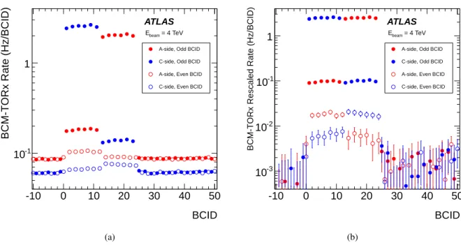
Figure 4: Single sided BCM-TORx rates of unpaired and empty bunches during periods with separated full energy beams before (a) and after (b) noise subtraction and rescaling to match the primary beam-background rates of both beams, as explained in the text. For clarity, signals in odd and even BCIDs are shown with different symbols. The unpaired bunches are all in odd BCIDs.

Since the afterglowBIB signal is very small, the overwhelming afterglow from the collisions prevents extracting it from stable-beam data. However, around 20 minutes of data at the start of each fill is obtained during the FLAT-TOP and SQUEEZE phases, in which the full-energy beams are separated and so there is no large afterglow from collisions. Figure4(a)shows the BCM-TORx rates for unpaired bunches and empty BCID around them, averaged over most fills with the 1368 colliding bunch structure. Only fills until the start of the BCM noise period are included. It is clearly seen that the background noise (BCIDs<1 and BCIDs>23) is low and BCID-independent.

In addition to the primary beam-gas signals, there are additional smaller signals in the upstream mod-ules. These are the hits from afterglowBIB. The afterglowBIBsignals are not easily identified in figure4(a) because they are barely above the noise level, which is different for the two sides. Also, the primary beam-gas signals themselves disagree by about 28%, i.e. much more than the efficiency difference of the two sides. This discrepancy reflects a real difference in beam background, possibly due to system-atically worse vacuum on side A. These arguments motivate processing the data by first subtracting the background noise and then rescaling one beam such that the primary BIB signals match. For each beam the noise level is determined as an average over 20 empty BCIDs preceding the first unpaired bunch. The rates in BCID 13–24 are multiplied by a factor of 1.28 in order to bring the primary BIB signals on the two sides into agreement.

The rates after these adjustments are shown in figure4(b), where two levels of signal rate in odd BCIDs on sides A and C are seen to match each other. The perfect agreement of the second level, around 0.1 Hz/BCID, after simply matching the primary BIB rates (∼2.5 Hz/BCID) on the two sides, means that it is proportional to the primary BIB rate at a level of 3.9% thereof, which leaves little doubt about its interpretation as afterglowBIBsignals.

In figure4(b)the factor 1.28 is applied also to the empty (even) BCIDs in the range 14–24 between beam-2 bunches. It is not evident if this is justified since the origin of the signals in them is not certain. A contribution from beam-1 ghost charge cannot be excluded. The statistical uncertainties on those points are large enough for the two sides to agree both with and without scaling.

In order to avoid confusion between afterglowBIB, which is important only because of its correlation with BIB events, and the much more significant level of afterglow from pp collisions, the latter will be referred to as afterglowpp.

The excellent time resolution of the BCM signal and data acquisition system enabled the arrival time of the background to be measured precisely. By exploiting the fine time binning of the recorded BCM signal, the existence of an afterglowBIBtail was verified and its shape was studied in detail. Figure5shows the time distributions in two BCM modules in events triggered by the L1_BCM_AC_CA trigger on unpaired isolated bunches of either beam. For beam-1 a pronounced early peak on the A-side is observed in figure5(a), corresponding to the background associated with the incoming bunch. It is followed by a long tail, consistent with afterglowBIB. Beam-1 exits on the C-side and correspondingly the peak appears around bin 43, i.e. ‘in-time’ with respect to the nominal collisions, again followed by a tail due to afterglowBIB. In figure5(b)similar structures are seen for beam-2, but on the opposite sides.

BCM time bin 0 10 20 30 40 50 60 protons] 11 Rate [Hz/10 7 − 10 6 − 10 5 − 10 4 − 10 3 − 10 2 − 10 1 − 10 1 10 2 10 =4 TeV beam E

Beam-1 UnpairedIso BCIDs before 27 Oct L1_BCM_AC_CA BCM A y+ BCM C y+ t [ns] 10 − −5 0 5 10 ATLAS (a) BCM time bin 0 10 20 30 40 50 60 protons] 11 Rate [Hz/10 7 − 10 6 − 10 5 − 10 4 − 10 3 − 10 2 − 10 1 − 10 1 10 2 10 =4 TeV beam E

Beam-2 UnpairedIso BCIDs before 27 Oct L1_BCM_AC_CA BCM A y+ BCM C y+ t [ns] 10 − −5 0 5 10 ATLAS (b)

Figure 5: Response of the BCM y+ station in the BCIDs defined for beam-1 (a) and beam-2 (b) in the events triggered by L1_BCM_AC_CA_UNPAIRED_ISO. Data with 1368 colliding bunches until the BCM noise period are used.

However, there are also some entries consistent with early hits in downstream modules. A flat, or slowly falling, pedestal is expected from noise and afterglow causing random triggers. But instead clear peak-like structures are seen in figure5, especially in unpaired BCIDs of beam-1. These can be attributed to ghost bunches in the other beam, but a detailed discussion is deferred to section9.

7. Background monitoring

7.1. Beam-gas events

The analysis of 2011 background data revealed a clear correlation of the beam background as seen by the BCM and the residual gas pressure reported by the gauges at 22 m. Using the data from a dedicated test fill without electron-cloud suppression by the solenoids at 58 m, the contribution of the pressure at 58 m to the observed background was estimated to be 3–4 % [1].

In 2012 no such dedicated test was performed, but the contributions of various vacuum sections were estimated by fitting the background (BIBBCM) data with a simple 3-parameter fit:

BIBBCM= A( f · p22 + (1 − f ) · p58) + b, (1)

where p22 and p58 are the pressures measured at 22 m and 58 m, respectively, and A, f and b are free parameters. The constant b is introduced to take into account any background not correlated with the two pressures included in the fit. Since BIBBCMis normalised by bunch intensity, the fit implies that also b is assumed to be proportional to beam intensity, which is a valid assumption if b is due to beam-gas further upstream. However, if a residual contribution comes from beam-halo losses or noise, it is not necessarily proportional to intensity.

The pressure values given by the three gauges, available at 22 m, were not always consistent. If inform-ation from an individual gauge was not received for a short time interval, the gap was bridged by using the last available value, provided it was in the same fill and not older than 10 minutes. Obviously erratic readings were rejected by requiring that the value was within a reasonable range (10−11– 10−6mbar).9 The pressure was determined by first taking the average of the pair of readings closest to each other and including the value from the third gauge only if it did not deviate by more than a factor of three from this pair-average. Such a three-gauge average was accepted in 97% of luminosity blocks and in only 0.3% of cases a two-gauge average was used. The number of cases that all gauges deviated by more than a factor of three from each other negligible. In 2.7% of luminosity blocks no valid pressure data could be determined and the luminosity block was ignored.

Figure6 shows the obtained fit parameters for the periods listed in table2 using either p22 only, i.e. f = 1.0, or a combination of p22 and p58 in Eq.1. It can be seen that the value of A, which corresponds to the absolute normalisation, is systematically lower for beam-2, which implies that for the same measured pressure there is less background from beam-2 than beam-1. The difference varies over the year, but is roughly 20% during the operation with 1368 colliding bunches (periods 3 and 4). The two sides of ATLAS are symmetric, so there is no obvious explanation why the backgrounds should be different. However, this difference in the fitted A is close to the 28% that was derived from figure4(b).

Ideally, the offset b should reflect how well the pressures alone describe BIBBCM. If b vanishes, it implies that there is no additional source contributing significantly, while b > 0 means that not all sources are included in the fit. Using p22 only results in b-values which are negative by a significant amount. These have no obvious physical interpretation and indicate that a linear fit using a single pressure is insufficient to describe the data. Using both, p22 and p58, clearly improves the model and results in b-values more consistent with zero.

Beam period

1 2 3 4

Fitted amplitude (A)

9 10 Beam-1, p22 Beam-2, p22 Beam-1, p22&p58 Beam-2, p22&p58 ATLAS

(a) Beam period

1 2 3 4 F it te d o ff s e t (b ) -0.2 -0.15 -0.1 -0.05 0 0.05 0.1 0.15 0.2 Beam-1, p22&p58 Beam-2, p22&p58 Beam-1, p22 Beam-2, p22 ATLAS (b) Beam period 1 2 3 4 Fitted p22 fraction (f) 0.86 0.87 0.88 0.89 0.9 0.91 0.92 0.93 0.94 0.95 0.96 ATLAS Beam-1, p22&p58 Beam-2, p22&p58 (c)

Figure 6: Parameters A (a), b (b) and f (c), resulting from the fit of equation1to data in periods 1–4, as detailed in table2.

The fraction f indicates how large a role p22 plays in explaining the observed background. The values gradually decrease during the year, but remain in a band of 90 ± 4%, confirming the result for 2011 operation, that the background seen by the BCM is strongly correlated with the pressure at 22 m.

Figure7 shows the intensity normalised BCM backgrounds for both beams separately before and after scaling with the residual pressures using a fit with p22 and p58 and parameter values shown in figure6. It should be remarked, however, that a similar plot using only p22 for scaling would be almost indistin-guishable from figure7(b). By construction, the scaling with equation1will result in an average of 1.0 in figure7(b). The remarkable feature is that by this scaling the fill-to-fill scatter is almost entirely removed, despite the fact that the parameters are fitted over four long periods, covering most of the year.

The background estimates for beam-1 and beam-2, shown in figure7(a), for the period with 1368 colliding bunches10lead to a beam-1/beam-2 ratio of 1.21 ± 0.17, which is perfectly consistent with the difference obtained before for the fitted parameter A. This ratio is also consistent with the factor 1.28 derived from non-colliding beam data in section6, which suggests that vacuum conditions, i.e. beam-gas event rates, do not significantly change when beams are brought into collision. Since neither figure4, nor figure7(a), involves a pressure measurement, these good agreements suggest that the difference observed in parameter A is not caused by different calibration of the gauges, but by a real difference in backgrounds. One possibility is that the pressure on side A has a different profile than that on side C and therefore the pressure gauges at 22 m do not have the same response in terms of average pressure in the region that contributes to the background.

7.2. Ghost collisions

The rate of ghost collisions, i.e. pp-collisions in encounters of unpaired and ghost bunches, can be estim-ated from the rate of events recorded by the L1_J10 and L1_BCM_Wide triggers in unpaired bunches. An independent method is to use the luminosity data from the BCM, which are recorded at high rate independently of the ATLAS trigger. In particular, the single-sided BCM event counting, BCM-TORx,

Date [UTC] 20/04/12 20/05/12 19/06/12 19/07/12 18/08/12 17/09/12 17/10/12 16/11/12 16/12/12 B C M b a c k g ro u n d [ H z /1 e 1 1 p ro to n s ] -1 10 1 10 No pressure scaling

Period 1, beam-1 Period 1, beam-2

Period 2, beam-1 Period 2, beam-2

Period 3, beam-1 Period 3, beam-2

Period 4, beam-1 Period 4, beam-2

ATLAS = 4 TeV beam E (a) Date [UTC] 20/04/12 20/05/12 19/06/12 19/07/12 18/08/12 17/09/12 17/10/12 16/11/12 16/12/12

Pressure-normalised BCM background [arb. units]

1 10

Scaled with p22 and p58

Period 1, beam-1 Period 1, beam-2

Period 2, beam-1 Period 2, beam-2

Period 3, beam-1 Period 3, beam-2

Period 4, beam-1 Period 4, beam-2

ATLAS = 4 TeV

beam

E

(b)

Figure 7: BCM background rate for both beams normalised by bunch intensity (a) and after an additional normal-isation with the pressures at 22 m and 58 m (b) using Eq.1with the parameters as shown in figure6. The shaded area indicates the period when the BCM was noisy.

as described in section4.1 can be used. In the following, both methods will be presented and results compared.

Ghost collision rates from recorded events

From June 2012 onwards L1_BCM_Wide and L1_J10 were both run without prescale on unpaired isol-ated and unpaired non-isolisol-ated bunches. A significant fraction of the raw L1_BCM_Wide and L1_J10 trigger rates in unpaired bunches are due to accidental coincidences or, in the case of the latter, fake jets

BCID 5 10 15 20 protons] 11 Rate [Hz/10 3 − 10 2 − 10 1 − 10 1 10 3318 ≤ Beam-1, LHC Fill 3318 ≤ Beam-2, LHC Fill 3318 ≤ Beam-1, LHC Fill 3318 ≤ Beam-2, LHC Fill vertex veto vertex required L1_BCM_Wide =4 TeV beam E ATLAS (a) BCID 5 10 15 20 protons] 11 Rate [Hz/10 3 − 10 2 − 10 1 − 10 1 10 3318 ≤ Beam-1, LHC Fill 3318 ≤ Beam-2, LHC Fill 3318 ≤ Beam-1, LHC Fill 3318 ≤ Beam-2, LHC Fill 3319 ≥ Beam-1, LHC Fill 3319 ≥ Beam-2, LHC Fill L1_J10 =4 TeV beam E vertex veto vertex required ATLAS (b)

Figure 8: Left: rate of L1_BCM_Wide triggered events in unpaired BCIDs for the period prior to swapping the unpaired bunches. The solid symbols show the rate after vertex requirement and the open symbols with a vertex veto. Right: rate of L1_J10 triggered events in the same period, and after swapping the unpaired trains.

due to BIB muons. In this analysis ghost collisions are selected offline from the recorded event data by requiring the presence of a reconstructed vertex in a volume consistent with the luminous region and with at least two associated tracks. In order to estimate the rates correctly, the vertex reconstruction efficiency has to be known. A method for estimating this from data for L1_BCM_Wide will be presented. Lu-minosity blocks, or entire fills, that do not meet general data quality requirements are removed from the analysis.

Figure8(a) shows the L1_BCM_Wide rates for events with and without a reconstructed vertex. The asymmetry of the ghost collision rate is striking. As expected, the rate is much higher for lower isolation – but only for the first unpaired train, i.e. beam-1. For the second train, comprising unpaired bunches in beam-2, the rates remain high even for isolated bunches. This asymmetry arises from the beam extraction from the PS, where the kicker is timed to the start of the unpaired train, but will also extract any possible trailing ghost bunches. As a result the unpaired trains systematically have more intensity in trailing than heading injected ghost bunches. The L1_J10 rates shown in figure8(b) confirm this shape. The plots also show that the unpaired isolated definition of having no bunch within 3 BCID in the other beam is adequate for the first train, while it includes a non-negligible tail of ghost collisions in the second train. This feature is preserved also after swapping the unpaired trains late in 2012, i.e. depends on the order of the trains and not on the beam.

The ghost collision rates seen in figure8are a product of ghost and unpaired bunch intensities in colliding RF buckets. These quantities can be directly measured by the LDM and the results for one of the fills when the system was operational are shown in figure9. Figure9(a) shows the charge in individual buckets and confirms the higher intensity of trailing injected ghost bunches and their 50 ns spacing. As explained in section3, this is due to spill-over in the PSB to PS injection. Figure9(b) shows the product of the bucket charges and largely confirms the shape seen in figure8. The small differences, especially for bucket 101 (BCID 11), are likely to be explained by fill-to-fill differences, since figure9 shows a single fill, while

RF bucket number

-100 -50 0 50 100 150 200 250 300 350

Bucket charge [Fraction of beam]

-12 10 -11 10 -10 10 -9 10 -8 10 -7 10 -6 10 -5 10 -4 10 -3 10

Beam-1 unpaired Beam-1 ghosts at 50ns Other beam-1 ghosts

Beam-2 unpaired Beam-2 ghosts at 50ns Other beam-2 ghosts

(a)

RF bucket number

-100 -50 0 50 100 150 200 250 300 350

LDM Intensity product [arb. units]

-13 10 -12 10 -11 10 -10 10

Beam-1 unpaired * Beam-2 ghost Beam-2 unpaired * Beam-1 ghost

(b)

Figure 9: Charge in individual RF buckets (a) as measured by the LDM in LHC fill 3005. The buckets corresponding to the 50 ns beam structure are shown by the larger symbols. The signal of each bucket has been normalised by the sum of signals from all buckets of the beam. The product (b) of the bucket charges in beam-1 and beam-2.

figure8is a long-term average. The point in RF-bucket 81 falls into the LDM trigger reset and had to be estimated from the value in bucket 101 using the ratio of the corresponding positions in front of other bunch-trains.

The rates with vertex veto, shown in figure8, are almost BCID-independent, consistent with their origin being random coincidences of hits – or noise in the case of jets – which are distributed uniformly in time. However, a barely visible hump in the centre (around BCID 11) can be identified, which is due to real collisions where vertex reconstruction has failed. Assuming that the probability of fake vertex recon-struction and the vertex reconrecon-struction inefficiency are both small, the latter can be estimated from the

Date [UTC]

31 Dec 01 Apr 01 Jul 01 Oct 31 Dec

protons]

11

Ghost collision rate [Hz/10

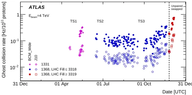
2 − 10 1 − 10 1 Unpaired swapped 1331 3318 ≤ 1368, LHC Fill 3319 ≥ 1368, LHC Fill 1331 3318 ≤ 1368, LHC Fill 3319 ≥ 1368, LHC Fill TS1 TS2 TS3 =4 TeV beam E BCM_Wide J10 ATLAS

Figure 10: Ghost collision rate in unpaired bunches in the 2012 data, estimated from events triggered by L1_BCM_Wide and L1_J10 triggers. In both cases the presence of at least one reconstructed vertex is required. The early BCM points are not included, since the device was not properly timed in. The technical stops are indicated in the plot.

relative sizes of the small and the large peaks in figure8(a). This yields an estimate of 1.1 % for the vertex reconstruction inefficiency. It must be emphasised, however, that this is the value with respect to collision events seen by the BCM and not a global inefficiency of ATLAS vertex reconstruction. Furthermore, a comparison of the flat tails in figure8(a), taking into account this inefficiency, provides an estimate of 1.27 for the beam-1/beam-2 ratio of BIB, which is perfectly consistent with the factor 1.28 derived in section6and 1.20 ± 0.17 found in section7.

The ghost collision rate during 2012 operation is shown in figure10, where it can be seen that the rate is rather constant until TS3 but rises steeply thereafter. L1_BCM_Wide and L1_J10 rates exhibit a similar rise, both in terms of shape and relative magnitude. Since the BCM and the calorimeters are totally independent and look at very different observables, it is not conceivable that the rise would be due to an increase of some random contribution. Thus, the identical rise must mean that the intensity of injected ghost bunches, colliding with the unpaired bunches, increased rapidly after TS3.

Ghost collision rates from luminosity data

The single-sided event rate, BCM-TORx, is composed of three contributions

Rate= Collisions + BIB + Pedestal, (2)

where the last term is defined to include both instrumental noise and afterglowpp. As shown in figure3 this pedestal can be estimated from the BCID before the unpaired bunch.

Prompt secondaries from upstream BIB events will not be counted in the upstream detector, since they arrive before the BCM-TORx window is open. A possible contribution of backscattering from beam-gas

events to upstream detectors is strongly suppressed by timing and the good vacuum close to the IP. The only process, besides pp-collisions, which can give in-time hits in upstream detectors is the afterglowBIB, discussed in section6. From this argumentation, and Eq.2, it follows that after pedestal subtraction, essentially all of the rate observed for unpaired bunches in the upstream BCM detector must be due to ghost collisions and afterglowBIB, the latter being proportional to the primary BG signal seen in the downstream modules.

The procedure to separate the single-side BCM rate into its three components, and the results obtained, are illustrated in figure11. In figure11(a) the open symbols indicate that the raw BCM-TORx rate is dominated by the pedestal and the other contributions are barely visible. A clear structure, resembling figure8(a)appears when the pedestal is subtracted, so that the data contain only beam-background and ghost collisions. The downstream modules are timed to see the primary BIB and ghost collision products emitted in the direction of the unpaired bunch, while the upstream modules see the ghost collision sec-ondaries emitted in the direction of the ghost bunch and a contribution from afterglowBIB. In figure4(b) the latter was estimated to be a fraction f = 0.039 of the primary BIB signal. Thus the rates seen in the upstream (Ru) and downstream (Rd) detectors can be written as:

Ru = f B + G (3)

and

Rd= B + G, (4)

where B stands for the primary rate from BIB and G for the rate from ghost collisions and the detection efficiencies are assumed to be identical on both sides. The equations can be solved to yield

B= Rd− Ru

1 − f (5)

and

G= Ru− f Rd

1 − f . (6)

It is worth to note that the value of f is small and in the limit f → 0 the equations simplify to G = Ru and B= Rd− Ru, i.e. the upstream detector measures the ghost collision rate and the difference between downstream and upstream detectors gives the rate due to BIB. Figure11(b) shows all the background components separated.

Figure12 compares the BCM-TORx rates, i.e. the components of Eqs.3and4, due to ghost collisions (G), BIB (B) and afterglowBIB( f B) for all fills in 2012 which had 1368 colliding bunches. It can be seen that for most of the year, beam-gas and ghost collisions, i.e. genuine luminosity, contribute about the same amount to the BCM-TORx rate in unpaired bunches, but at the very end of the year there is a steep rise in the ghost collision rate and it becomes the dominant contribution. This result implies that if the rate seen in unpaired bunches is used as background correction to a BCM-based luminosity measurement in a high-luminosity fill, a detailed decomposition, as described here, must be done in order to separate out the ghost collision contribution.

Having presented two different methods to monitor ghost collision rates, a comparison between the results remains to be done. The fake ghost collision triggers, i.e. coincidences without a real collision, are a sum of many independent contributions and therefore provide the most sensitive basis for comparison. Assuming that B in Eq.5and the pedestal are uncorrelated between sides A and C, the random coincid-ence rates can be obtained by simple multiplication. The rate of these fake ghost collisions should be the

BCID -5 0 5 10 15 20 25 30 B C M -T O R x R a te [ H z /B C ID ] -2 10 -1 10 1 10 2 10 Fill 2843

Side A with pedestal Side C with pedestal Side A no pedestal Side C no pedestal ATLAS = 4 TeV beam E (a) _BCID 0 5 10 15 20 25 protons] 1 1 B C M -T O R x R a te [ H z /1 0 -2 10 -1 10 1 10 2 10 Fill 2843 Side A pedestal Side C pedestal Ghost collisions Side A BIB Side C BIB ATLAS = 4 TeV beam E (b)

Figure 11: The procedure of separating the background components in unpaired bunches. The open symbols in plot (a) show the total single-sided rate seen by the BCM while the solid symbols show the data after subtraction of the background and restricted to the BCID-range of the unpaired punches. Plot (b) shows the three background components separated, as explained in the text.

same as that obtained from the event-by-event analysis after applying a vertex veto. Since the pedestal is uniformly distributed in time, the different window widths of the BCM_Wide trigger and the luminosity trigger have to be taken into account, as detailed in appendixA.

The problematic component of the non-collision L1_BCM_Wide rate is the afterglowBIB, because it does not fulfil the requirement of being uncorrelated with B on the other side. Unfortunately figure4(b)only determines the total afterglowBIBrate to be about 3.9% of B but does not give any information about the correlation between B and afterglowBIBsignals, i.e. how often the latter coincides with the former. If the L1_BCM_AC_CA triggered sample were an unbiased subset of BIB events giving a signal in the downstream detector, the correlation could be estimated as the fraction of L1_BCM_AC_CA triggered events, which are also triggered by L1_BCM_Wide, but have no vertex. However, the events selected by L1_BCM_AC_CA are likely to be biased towards higher multiplicities with respect to BIB events giving only downstream hits. A higher multiplicity will also imply a higher likelihood to obtain a L1_BCM_Wide trigger due to an associated afterglowBIBhit. Thus the observed fraction of 1.3% should be considered an upper limit.

A better method to estimate the correlation is to require that the estimated rate agrees with that of events recorded by the L1_BCM_Wide trigger, after applying a vertex veto. The best match over all 2012 is obtained when 0.9% of the downstream beam-gas hits are assumed to be in coincidence with an upstream afterglowBIBhit. Being slightly lower than the 1.3 %, this value is considered perfectly reasonable. When this coincidence fraction of 0.9% is applied to all fills of 2012 with 1368 colliding bunches, the non-collision BCM_Wide rate estimates shown in figure13are obtained. The plot is consistent with the as-sumption that most of this rate comes from a coincidence formed by BIB and its associated afterglowBIB. The open circles in figure13are the sum of the three other components shown with the addition of 1.1%

Date [UTC]

protons]

1

1

B

C

M

-T

O

R

x

R

a

te

[

H

z

/1

0

-2

10

-1

10

1

10

Ghost collision

BIB

Upstream afterglow

ATLAS

E

= 4 TeV

Figure 12: The BCM-TORx rate in unpaired bunches due to BIB, afterglowBIBand ghost collisions for all 2012 fills

with 1368 colliding bunches. Only the first 100 LB (∼ 100 minutes) of stable beams in each fill have been used in order to remove fill-length dependence.

of ghost collisions in order to take into account the vertex reconstruction inefficiency. Inclusion of this small fraction of ghost collisions is needed to describe the rise towards the end of the year. An agreement of the open circles and open squares is enforced on average by the matching of the data, as described above. This procedure, however, does not constrain agreement of the fill-to-fill fluctuations or the slight rise over the year. For both very good consistency between the two methods is observed.

Date [UTC] 19/06/12 19/07/12 18/08/12 17/09/12 17/10/12 16/11/12 16/12/12 protons] 1 1 BCM_Wide Rate [Hz/10 -4 10 -3 10 -2 10 -1 10 Ebeam = 4 TeV Total non-collision coincidences BIB BIB-Afterglow Noise-Noise coincidences Noise-BIB coincidences BCM_Wide events, no vertex

ATLAS = 4 TeV

beam

E

Figure 13: The total non-collision rate in the BCM_Wide trigger for 2012 LHC Fills with 1368 colliding bunches and the individual contributions to this rate. The open circles include a contribution of real ghost collisions due to the 1.1% vertex inefficiency. The jump in the pedestal-related components is due to the appearance of the BCM noise (shaded area), which then gradually decreased. Only the first 100 LB (∼ 100 minutes) of stable beams in each fill have been used in order to remove fill-length dependence due to the decreasing afterglow.

8. Fake jets

Muons can emerge from the particle showers initiated by beam gas interactions or scattering of the beam halo protons at limiting apertures of the LHC. Such BIB muons, with energies potentially up to the TeV range, may enter the ATLAS calorimeters and deposit energy which is then reconstructed as a fake jet. The simulations of BIB show that the high-energy muons leading to fake jets at radial distances of R > 1 m, originate from the tertiary collimators or, in the case of beam-gas collisions, even further away [1,11]. Nearly every physics analysis in ATLAS requires good quality jets with the pile-up contribution sup-pressed and non-collision backgrounds removed. In reference [1] various sets of jet cleaning criteria were proposed to identify NCB. Since then, these have been commonly used in ATLAS analyses. While calori-meter noise appears at a rate low enough to not significantly increase the trigger rate, caloricalori-meter hot cells, BIB and CRB-muons may take up a significant fraction of the event recording bandwidth. The number of events triggered by a fake jet and entering a given analysis, strongly depends on the event topology considered. Single-jet selections are most likely to pick up a fake jet on top of minimum-bias collisions that happen during every crossing of two nominal bunches. Therefore, analyses with jets and missing transverse momentum (Emiss_T ) in the final state, such as the mono-jet analysis [13], crucially depend on an efficient jet-cleaning strategy. More complicated topologies will include NCB only if it is in combination with other hard collision products.

This section reports on the observation of fake jets due to BIB muons in unpaired bunches as well as the ones extracted from collision data by inverting the jet cleaning selection. In addition, the rates of fake jets due to CRB muons are compared to a dedicated Monte Carlo simulation. Finally the rates of fake jets due to BIB and CRB are compared as a function the pTof the reconstructed jet.