Biological and bio-inspired morphometry as a route to tunable and enhanced materials design

(1)

Biological and Bio-Inspired Morphometry as a Route

to Tunable and Enhanced Materials Design

by

Swati Varshney

BS Chemistry, Carnegie Mellon University (2010)

MPhil Micro- & Nanotechnology Enterprise, University of Cambridge (2011)

Submitted to the Department of Materials Science and Engineering

in partial fulfillment of the requirements for the degree of

Doctor of Philosophy in Materials Science and Engineering at the

MASSACHUSETTS INSTITUTE OF TECHNOLOGY

June 2016

Author... Department of Materials Science and Engineering April 4, 2016

Certified by... Mary C. Boyce Ford Professor of Mechanical Engineering Thesis Supervisor

Certified by... Christine Ortiz Morris Cohen Professor of Materials Science and Engineering Thesis Supervisor

Accepted by... Donald R. Sadoway Chair, Departmental Committee on Graduate Students

(2)

(3)

3

Biological and Bio-Inspired Morphometry as a Route

to Tunable and Enhanced Materials Design

by

Swati Varshney

Submitted to the Department of Materials Science and Engineering on April 4, 2016 in partial fulfillment of the requirements for the degree of Doctor of Philosophy

Abstract

Structural materials in nature integrate classical materials selection rules with morphometry (geometry or shape-based rules) to create high-performance, multi-functional structures that exhibit tunable properties through extraordinary complexity, hierarchy, and precise structural control. This thesis explores the use of morphometry as a materials design parameter through the development of bio-inspired, flexible composite armor based on the articulated exoskeleton of an armored fish, Polypterus senegalus, which achieves uniform coverage and protection from predatory threats without restricting flexibility. First, the functional implications of shape and shape variation are examined as materials design parameters within the biological exoskeleton using a new method that integrates continuum strain analysis with landmark-based geometric morphometric analysis in 2D and 3D. Bioinspired flexible composite prototypes are fabricated using multi-material 3D printing and tested under passive loading (self-weight) and active loading (bending) to examine how the shape of scales contributes to local, interscale mobility mechanisms that generate anisotropic, global mechanical behavior. With one prototype design scheme, a wide array of mechanical behavior is generated with stiffness ranging over several orders of magnitude, including ‘mechanical invisibility’ of the scales, showing how

morphometry can tune flexibility without varying the constituent materials. Finally, finite element models simulating the bending experiments are created to establish a computational framework for analyzing the mechanical response of the prototypes. The finite element models are then extended to examine the effect of different loading conditions, scale morphometry, multi-material architecture, and constituent material properties. The results show how

morphometric-enabled materials design, inspired by structural biological materials, can allow for tunable behavior in flexible composites made of segmented scale assemblies to achieve enhanced user mobility, custom fit, and flexibility around joints for a variety of protective applications.

Thesis Supervisor: Mary C. Boyce Title: Ford Professor of Engineering Thesis Supervisor: Christine Ortiz

(4)

(5)

5

Acknowledgements

I would first like to thank my thesis advisors, Professor Christine Ortiz and Professor Mary C. Boyce, for sharing with me their passion for bio-inspired engineering and the mechanics of materials. Their encouragement to craft new methods to tackle emerging problems has shaped me into a multi-disciplinary researcher with the courage to think outside the box and push the boundaries of materials science and engineering. I appreciate the independence they bestowed upon me to pursue new areas of research in depth across multiple fields of study.

I especially thank Katia Zolotovsky, a PhD candidate in the Department of Architecture, who has worked closely with me on many aspects of my thesis research. Her skills in 3D printing and computational modeling have been invaluable, and I am indebted to her for teaching me how to approach problems from the perspective of a designer in addition to that of an engineer.

I am grateful to the academic mentors who have guided my research. Dr. Ming Dao provided advice and encouragement for my finite element simulations. Dr. Simon Bellemare issued me hands-on experience analyzing the mechanics of structural materials in commercial applications. Professor Neri Oxman contributed insight into the world of multi-material fabrication techniques. My thesis committee members, Professor Darrell Irvine and Professor Michael Rubner, always had constructive feedback to re-invigorate my enthusiasm for delving deeper into my research. Professor Rick McCullough has served as the perfect amalgam of a teacher, mentor, and friend since my undergraduate research days.

I am filled with gratitude for the support of my colleagues in the Ortiz Group and Boyce Group during my time at MIT: Erica Lin, Narges Kaynia, Eric Arndt, Ling Li, Matt Connors, Mark Guttag, Shabnam Ardakani, Cody Ni, Hansohl Cho, Ashley Durand, Juha Song, and Yaning Li. I cannot forget Steffen Reichert, who graduated before I joined the group, but who laid the groundwork for the shape analysis and prototyping that went into my research. I also thank Teri Hayes, Jessica Landry, and Esther Schwartz for handling administrative activities related to my research. I must also acknowledge Dr. Mike Esmail whose veterinary expertise was invaluable in caring for my fish.

Finally, I am thankful for the unwavering support of my friends and family. I thank Greg, for believing in me and for always going the extra mile to keep a smile on my face; Lauren, for being the best best friend ever; Kelsey, for being an amazing roommate and moreover an

incredible inspiration to show how far hard work, dedication, and genuine kindness can take you; Andrew, for countless espressos, fancy teas, and Starbucks runs; my skydiving friends, for challenging my mind and body through extreme sports, epic shredding, and sick swoops; the many friends who have been by my side through the years, including Kavita, Anna L, Anna Q, Maryanna, Becca, Erika, Ryan, Saskia, and Tucker; my brother, Vivek, for his willingness to drop anything and everything when I need help; and last but not least, my parents, for their unconditional love and support since day one.

(6)

6 For my parents

(7)

7

List of Figures

Figure 1.1: The protection vs. flexibility tradeoff in current armor technologies [42-46, 52]. ... 24 Figure 1.2: The hierarchical materials-morphometric design principles of the P. senegalus

exoskeleton. (a) X-ray microcomputed tomography (µCT) reconstruction of a P. senegalus specimen, adapted from [58]. (b) Anesthetized P. senegalus specimen (body length = 219 mm) exhibiting large bi-directional body curvature in axial bending [59]. (c) Optical micrographs of a single scale cross-section showing the quad-layered structure [30, 60]. (d) Scanning electron micrograph (SEM) of ganoine nanocrystals [30]. (e) SEM of the dentin layer [61]. (f) Backscatter SEM (BSEM) of isopedine cross-section [60]. (g) Atomic force micrograph (AFM), height-image, of a polished cross section of the bony plate [61]. (h) Optical micrographs of 1N and 2N microindentations on scale surface showing circumferential cracking [30]. (i) BSEM showing crack arrest at the ganoine-dentin junction [30]. (j) Schematic of the helical arrangement of scales showing the paraserial axis (red) and interserial axis (black) [55]. (k) Schematic showing the local articulation of scales. (l) µCT reconstruction of a single scale, interior (left) and exterior (right) views [62]. (m) SEM of outer scale surface [30]. (n) SEM of inner scale surface [30]. (o) Schematic of the articulated, paraserial peg-and-socket joint [62]. (p) Schematic of the sliding, interserial overlap joint [62]. (q) Schematic of the interior view of the local assembly of scales, showing sites of attachment of Sharpey’s fibers (asf) and attachment of stratum compactum (asc), as well as the fibers of the stratum compactum (sc) that run along the paraserial (ps) and interserial (is) axes [55]. (r) SEM of the interior of the scale showing the site of attachment of the stratum compactum to the axial ridge of the scale [55]. (s) SEM of stratum compactum [55]. (t) SEM showing Sharpey’s fibers connecting the peg and socket of adjacent scales [55]. ... 26 Figure 1.3: Prior research in developing P. senegalus -inspired armor prototypes. (a) Two

scales that have been unitized, enlarged, and 3D printed with plaster [59]. (b) Single scale incorporating material heterogeneity through the scale’s porous architecture [82]. (c) Monolithic semi-helical ring structures [59]. (d) Simplified scale design allowing two rotational degrees of freedom at the paraserial and interserial joints [59]. (e) Simplified scale design from (d) 3D-printed and assembled with rubber bands to mimic the fibrous interconnections [59]. (f) 1×2 arrays of scales incorporating compliant material elements in

(11)

11

the peg-and-socket interconnections (top) and the attachment site to the underlying substrate (bottom) using multimaterial 3D printing [59]. (g) 5×5 flexible scale assembly [59]. ... 30 Figure 2.1: The P. senegalus exoskeleton. (a) μCT reconstruction (18 µm scan resolution) of

the P. senegalus exoskeleton used in the morphometric analysis, and (b) μCT reconstruction of a P. senegalus specimen in a fully extended configuration (95 µm scan resolution) [10]. Images show the paraserial axis of scale articulation (column), the interserial axis of scale overlap, the anterior-posterior row, dorsal and ventral midlines of mirror symmetry, and pectoral fin. Select scales are numbered by column and row number (C#R#). The asterisked scale (C9R5) in (a) is used in Fig. 2.2. ... 37 Figure 2.2: μCT reconstruction (10 µm scan resolution) of a single P. senegalus scale (C9R5),

(a) interior and (b) exterior views. Geometrical features are labeled: peg (P), socket (S), anterior process (AP), axial ridge (AR), and anterior margin (AM). The 20 LMs used for morphometric analysis are shown (red dots) and described in Table 2.1. The x-y coordinate axis is defined with the x-axis aligned with the scale’s paraserial axis, and y-axis defined 90° perpendicular to the x-axis in the plane of the scale. Two morphometric parameters are shown: peg tip angle (γ) and anterior process angle (θ). ... 38 Figure 2.3: Selection criteria for the number of LMs used in the morphometric analysis. (a)

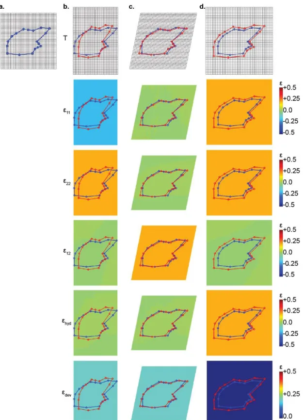
Single scale (C31R10) with 60 LMs placed around outer surface, numbered in order of their selection for calculating polygonal area. LMs in red represent the first 18 LMs shown in Fig. 2.2. (b) Plot of polygonal area versus number of landmarks selected to define the outline of the scale, for five different scales in different regions in the P. senegalus exoskeleton. ... 39 Figure 2.4: Landmark-based GM and continuum strain analysis of affine transformations. (a)

Reference scale geometry (blue) mapped to an undeformed grid. (b-d) Transformation grids (T) and strain plots mapping the components of strain tensor (ε11, ε22, and ε12), hydrostatic

strain (εhyd) and the norm of the deviatoric strain tensor (εdev) for affine transformations (red)

applied to the reference geometry (blue): (b) compression (ε11 = -ε22 = -0.2), (c) simple shear

(ε12 = +0.2) and (d) uniform scaling (ε11 = ε22 = +0.2)... 42 Figure 2.5: Transformation grids (T) and strain plots mapping the shear component of strain

(ε12) for a series of affine shear operations (red) applied to the reference geometry (blue): (a) ε12 = -0.5, (b) ε12 = -0.4, (c) ε12 = -0.3, (d) ε12 = -0.2, (e) ε12 = -0.1, (f) ε12 = 0.0, (g) ε12 = +0.1,

(12)

12

(h) ε12 = +0.2, (i) ε12 = +0.3, (j) ε12 = +0.4, (k) ε12 = +0.5, and (l) plot of the total strain energy

(U, normalized by maximum value) vs. shear strain. ... 43 Figure 2.6: Scale shape variation from anterior to posterior. (a) μCT reconstruction of scales

within a single row (R6) of the P. senegalus specimen, every fifth scale shown (15 µm scan resolution). (b) Schematic of the exoskeleton illustrating the row of scales used for the analysis. (c) Transformation grids (T) compare the geometry of three scales (C5R6, C25R6, and C45R6; in red) to the reference geometry (blue). Strain plots map the components of the strain tensor (ε11, ε22, and ε12), hydrostatic strain (εhyd) and norm of the deviatoric strain tensor

(εdev) for each grid element. ... 46 Figure 2.7: Scale shape variation from dorsal to ventral. (a) μCT reconstruction of scales within

a single column (C22) of the P. senegalus specimen, every other scale shown (15 µm scan resolution). (b) Schematic of the exoskeleton illustrating the column of scales used for the analysis. (c) Transformation grids (T) compare the geometry of three scales (C22R2, C22R8, and C22R14; in red) to the reference geometry (blue). Strain plots map the components of the strain tensor (ε11, ε22, and ε12), hydrostatic strain (εhyd) and norm of the deviatoric strain

tensor (εdev) at each grid point. ... 48 Figure 2.8: The P. senegalus pectoral fin and scale shape variation along a transition seam. (a)

μCT reconstruction of the left pectoral fin (8 µm scan resolution) highlighting a transition row segment. (b) Exterior (top) and interior (bottom) views of an articulated seam of scales connecting the main body to the pectoral fin. (c) Transformation grids (T) compare the geometry of three scales (P2, P4, and P6; in red) to the reference geometry (blue). Strain plots map the components of the strain tensor (ε11, ε22, and ε12), hydrostatic strain (εhyd) and

norm of the deviatoric strain tensor (εdev) at each grid point. ... 49 Figure 2.9: Boxplots for the range of values of morphometric parameters over the row, column,

and pectoral fin seam. γ and θ are normalized by 180°, and V and U are normalized by their maximum value over all scales (5.44 mm3_{and 2.1x10}10_{J, respectively) to generate unitless}

parameter values. Data are segmented into quartiles with no outliers. ... 50 Figure 2.10: Schematic of interscale mobility mechanisms. (a) A quad of scales showing

interserial and paraserial axis in native (resting) state. Motion of scales can be broken into four components: (b) interserial sliding, (c) interserial splay, (d) paraserial rotation, and (e) paraserial bending. ... 53

(13)

13

Figure 2.11: Recomposing morphometric variation by applying strain. (a) Transformation grid (T) and strain tensor components (ε11, ε22, and ε12) comparing a biological scale geometry

(C10R6, in red) to the reference geometry (blue). (b) Transformation grids resulting from the application of each component of the strain tensor (ε11, ε22, and ε12) found in (a) to the

reference geometry. Applying all three components of the strain tensor to the reference geometry recovers the geometry of the biological scale. ... 55 Figure 3.1: μCT reconstruction (10 µm scan resolution) of a single P. senegalus scale (C9R5)

(a) interior and (b) exterior views showing the 21 LMs (red dots) used in the 3D morphometric analysis, described in Table 3.1. The coordinate systems is defined from the centroid with the x-axis aligned with the scale’s paraserial axis, and y-axis defined 90° perpendicular to the x-axis in the plane of the scale, and the z-axis vertically through the thickness of the scale point to the exterior (top) surface of the scale. ... 59 Figure 3.2: Illustrations of the 3D morphometric parameters described in Table 3.2. ... 62 Figure 3.3: Morphometric parameters for the (a) row, (b) column, and (c) pectoral fin data

series. Central thickness (T), curvature (L), % scale volume reduction due to concavity of the anterior margin (AM%), and 3D strain energy (U) are plotted as unitless parameters normalized by their maximum value (left axis). Angle of interserial overlap (λ) is plotted in degrees (right axis). Volume of the base of the scale (VB), volume of the peg (VP) and volume of the anterior shelf (VAS) are stacked as area plots as a percentage of the total scale volume. Calculations for these parameters are presented in Table 3.2. ... 63 Figure 3.4: 3D morphometric analysis of the average scale variant (C30R6). (a) µCT

reconstruction of the scale. (b) Undeformed 3D grid. (c) Deformed 3D transformation grid showing scale geometry (red) compared to the reference geometry (blue). (d) 2D medial slices of the transformation grid in the XY, XZ, and YZ planes. (e) 3 XY slices. (f) 3 XZ slices. (g) 3 YZ slices. (h) Strain plots on medial XY, XZ, and YZ slides comparing the scale (red) to the reference (blue)... 65 Figure 3.5: 3D morphometric analysis of the anterior scale variant (C10R6). (a) µCT

reconstruction of the scale. (b) Undeformed 3D grid. (c) Deformed 3D transformation grid showing scale geometry (red) compared to the reference geometry (blue). (d) 2D medial slices of the transformation grid in the XY, XZ, and YZ planes. (e) 3 XY slices. (f) 3 XZ

(14)

14

slices. (g) 3 YZ slices. (h) Strain plots on medial XY, XZ, and YZ slides comparing the scale (red) to the reference (blue)... 66 Figure 3.6: 3D morphometric analysis of the tail scale variant (C50R6). (a) µCT reconstruction

of the scale. (b) Undeformed 3D grid. (c) Deformed 3D transformation grid showing scale geometry (red) compared to the reference geometry (blue). (d) 2D medial slices of the transformation grid in the XY, XZ, and YZ planes. (e) 3 XY slices. (f) 3 XZ slices. (g) 3 YZ slices. (h) Strain plots on medial XY, XZ, and YZ slides comparing the scale (red) to the reference (blue). ... 67 Figure 3.7: 3D morphometric analysis of the ventral scale variant (C22R14). (a) µCT

reconstruction of the scale. (b) Undeformed 3D grid. (c) Deformed 3D transformation grid showing scale geometry (red) compared to the reference geometry (blue). (d) 2D medial slices of the transformation grid in the XY, XZ, and YZ planes. (e) 3 XY slices. (f) 3 XZ slices. (g) 3 YZ slices. (h) Strain plots on medial XY, XZ, and YZ slides comparing the scale (red) to the reference (blue)... 68 Figure 3.8: 3D morphometric analysis of the pectoral fin scale variant (P6). (a) µCT

reconstruction of the scale. (b) Undeformed 3D grid. (c) Deformed 3D transformation grid showing scale geometry (red) compared to the reference geometry (blue). (d) 2D medial slices of the transformation grid in the XY, XZ, and YZ planes. (e) 3 XY slices. (f) 3 XZ slices. (g) 3 YZ slices. (h) Strain plots on medial XY, XZ, and YZ slides comparing the scale (red) to the reference (blue)... 70 Figure 4.1: Design and fabrication of P. senegalus-inspired flexible composite prototypes. (a)

Rendering of an abstracted scale geometry, showing the orientation of the paraserial and interserial axes and two controllable parameters: scale length (L) and scale height (H). Adapted from [1]. (b) Schematic of the multimaterial components of the articulated assembly, bottom view, adapted from [1]. (c) Top view of the prototype design. (d) Cross-sectional view of the prototype design. (e) 3D printed flexible composite prototype. (f) Close-up of the 3D printed prototype showing the orientation of the paraserial and interserial axes. ... 75 Figure 4.2: Experimental methods to analyze prototype behavior under passive loading. (a)

Setup of the curvature experiment. The prototype is draped over a curved mold. Rigid rods are inserted into three scales in a single line along the mold’s axis of curvature (y-axis). A

(15)

15

camera along the mold’s line of zero curvature (x-axis) captures the image in order to calculate the radius of curvature of the prototype (Rp) vs. radius of curvature of the mold

(Rm). (b) Setup of the joint degrees of freedom experiment. The prototype is draped over a

curved mold. Rigid rods are inserted into three scales, two along the paraserial axis and two along the interserial axis of the assembly. Cameras along the mold’s line of zero curvature (x-axis) and line of curvature (y-axis) capture images to calculate interscale angles. (c-d) Top-view schematics illustrating interscale angles between Rods 1-2 and Rods 1-3... 75 Figure 4.3: Anisotropy of prototype flexibility measured by radius of curvature. (a) Prototype

draped over a half-cylinder mold at orientation angle (α) = 0°. Lines show the curvature of the mold (white) and prototype (red). Inverse of curvature represents the radius of curvature of the prototype (Rp) and the radius of curvature of the mold (Rm = 120 mm). The prototype

exhibits different curvatures when rotated to (b) α = 30°, (c) α = 60°, (d) α = 90°, and (e) α = 120°. (f) Top view of the prototype in the α = 0° orientation. (g) Top view of the prototype in the α = 75° orientation. (h) Relative radius of curvature (Rp/Rm) vs. α for the prototype, a

variation with the halved length aspect ratio, a variation without the paraserial connections, and the substrate only without scales. Error bars represent standard deviation with N = 3 samples per prototype design. ... 77 Figure 4.4: Contribution of joint degrees of freedom to the prototype flexibility. (a) Schematics

of four joint degrees of freedom and their corresponding interscale angles. (b) Interscale angles vs. rotation angle (α) of the prototype. Error bars represent standard deviation for N = 3 samples. ... 78 Figure 5.1: Design and testing of flexible composite prototypes in bending. (a-f) Schematics

of the prototypes. Dashed lines represent the paraserial (ps) axis, interserial (is) axis, the angle (β) between the paraserial and interserial axes, and scale orientation angle (φ) of 0°, 30°, 60°, 90°, 120°, and 150°. (g) Optical photograph of the sample holder attached to the rods of the prototype and affixed to the plate of the Zwick. (h) Side-view of the φ = 60° sample loaded in concave bending at various vertical displacements (d), from left to right: d = 3 mm, d = 20 mm, d = 50 mm, and d = 80 mm. ... 83 Figure 5.2: Anisotropic stiffness of flexible composite prototypes in concave bending. (a)

Force-displacement curves for prototypes with φ = 0°, 30°, 60°, 90°, 120°, and 150°. (b) Normalized stiffness (K) of each phase of each prototype’s loading curve. Error bars

(16)

16

represent standard deviation with N = 3 samples per prototype orientation. ... 85 Figure 5.3: Schematics of the six interscale mobility mechanisms observed. ... 85 Figure 5.4: Orientation-dependent behavior of the scaled prototypes in concave bending. (a)

Photographs of φ = 0° sample: (i-ii) Vertical displacement (d) = 3 mm, side view and close up view of scales. (iii-v) d = 20 mm, side view, close up view of scales, and close up view of substrate. (vi-vii) d = 60 mm, side view and close up view of scales. (b) Photographs of φ = 30° sample: (i-ii) d = 3 mm, side view and close up view of scales. (iii-iv) d = 15 mm, side view and close up view of scales. (v-vi) d = 80 mm, side view and close up view of scale. (c) Photographs of φ = 60° sample: (i-ii) d = 4 mm, side view and close up view of scales. (iii-v) d = 50 mm and 80 mm, side view and close up view of scales. ... 86 Figure 5.5: Orientation-dependent behavior of the scaled prototypes in concave bending. (a)

Photographs of φ = 90° sample. (i-iii) Vertical displacement (d) = 15 mm, side view and corresponding close up views of scales. (iv-vi) d = 60 mm, side view, oblique view, and close up views of scales and substrate. (b) Photographs of φ = 120° sample. (i-ii) d = 4 mm, side view and close up view of scales. (iii-iv) d = 20 mm, side view and close up view of scales with d = 20 mm. (v-vi) d = 60 mm, side view and close up view of scales. (c) Photographs of φ = 150° sample. (i-ii) d = 4 mm, side view and close up view of scales. (iii-iv) d = 14 mm, side view and close up view of scales. (v-vi) d = 40 mm, side view and close up view of scales. ... 87 Figure 6.1: Finite element model design. (a) Simplified scale, (i) top view and (ii) side view.

(b) Grooved substrate, (i) top view for orientation angle (φ) = 60°, and (ii) side view with φ = 0° showing scales placed in the shallow groove, where red lines define the axial ridge of scales. (c) Assembly of parts for the model with φ = 60°. ... 93 Figure 6.2: Finite element results for concave bending. (a) Normalized stiffness (K) of each

phase of each finite element (FE) model and experiment (Exp.), N=3 and error bars represent standard deviation. (b) Interscale mobility mechanisms observed in the finite element models. From top to bottom, left: paraserial bending, interserial rotation, interserial splay; right: interserial sliding, paraserial rotation. ... 94 Figure 6.3: Stress plots (Mises) from the finite element simulations of flexible composite

prototypes in concave bending. (a) Stress plots from the φ = 0° model. (i) Front view at vertical displacement (d) = 3 mm. (ii) Front view at d = 9 mm. (iii) Back view at d = 9 mm.

(17)

17

(iv) Front view at d = 22 mm. (v) Scale bar. (b) Stress plots from the φ = 30° model. (i) Front views at d = 3 mm, (ii) d = 14 mm, and (iii) d = 33 mm. (iv) Scale bar. (c) Stress plots from the φ = 60° model. (i) Front views at d = 5 mm, (ii) d = 8 mm, and (iii) d = 38 mm. (iv) Scale bar. ... 95 Figure 6.4: Strain plots (logarithmic, max. principal) from the finite element simulations of

flexible composite prototypes in concave bending. (a) Strain plots from the φ = 0° model. (i) Back views at vertical displacement (d) = 3 mm, (ii) d = 9 mm, and (iii) d = 22 mm. (iv) Front view at d = 22 mm. (v) Scale bar. (b) Strain plots from the φ = 30° model. (i) Back views at d = 3 mm, (ii) d = 14 mm, and (iii) d = 33 mm. (iv) Close up view of the scale-substrate attachment at d = 33 mm. (v) Scale bar. (c) Strain plots from the φ = 60° model. (i) Back views at d = 5 mm, (ii) d = 8 mm, and (iii) d = 38 mm. (iv) Close up view of the scale-substrate attachment at d = 24 mm. (v) Scale bar. ... 96 Figure 6.5: Strain plots (logarithmic, components (LEij)) from the finite element simulations

in concave bending. (a) Strain plots from the φ = 0° model, back view at vertical displacement (d) = 9 mm: (i) LE11, (ii) LE22, (iii) LE33, (iv) axial strain scale bar, (v) LE12, (vi) LE13, (vii) LE23, and (viii) shear strain scale bar. (b) Strain plots from the φ = 30° model, back view at d = 14 mm: (i) LE11, (ii) LE22, (iii) LE33, (iv) axial strain scale bar, (v) LE12, (vi) LE13, (vii) LE23, and (viii) shear strain scale bar. (c) Strain plots from the φ = 60° model, back view at d = 38 mm: (i) LE11, (ii) LE22, (iii) LE33, (iv) axial strain scale bar, (v) LE12, (vi) LE13, (vii) LE23, and (viii) shear strain scale bar. ... 97 Figure 6.6: Stress plots (Mises) from the finite element simulations of flexible composite

prototypes in concave bending. (a) Stress plots from the φ = 90° model. (i) Front views at vertical displacement (d) = 12 mm, (ii) d = 43 mm, and (iii) d = 68 mm. (iv) Scale bar. (b) Stress plots from the φ = 120° model. (i) Front views at d = 3 mm, and (ii) d = 12 mm. (iii) Back view at d = 12 mm. (iv) Front view at d = 52 mm. (v) Scale bar. (c) Stress plots from the φ = 150° model. (i) Back view at d = 3 mm. (ii) Front views at d = 20 mm, (iii) d = 38 mm, and (iv) d = 55 mm. (v) Scale bar. ... 98 Figure 6.7: Strain plots (logarithmic, max. principal) from the finite element simulations of

flexible composite prototypes in concave bending. (a) Strain plots from the φ = 90° model. (i) Back views at vertical displacement (d) = 12 mm, (ii) d = 43 mm, and (iii) d = 68 mm. (iv) Front view at d = 68 mm, left side cropped. (v) Scale bar. (b) Strain plots from the φ =

(18)

18

120° model. (i) Back views at d = 3 mm, (ii) d = 12 mm, and (iii) d = 26 mm. (iv) Scale bar. (c) Strain plots from the φ = 150° model. (i) Back views at d = 3 mm, (ii) d = 12 mm, and (iii) d = 38 mm. (iv) Scale bar. ... 99 Figure 6.8: Strain plots (logarithmic, components (LEij)) from the finite element simulations

in concave bending. (a) Strain plots from the φ = 90° model, back view at vertical displacement (d) = 43 mm: (i) LE11, (ii) LE22, (iii) LE33, (iv) axial strain scale bar, (v) LE12, (vi) LE13, (vii) LE23, and (viii) shear strain scale bar. (b) Strain plots from the φ = 120° model, back view at d = 12 mm: (i) LE11, (ii) LE22, (iii) LE33, (iv) axial strain scale bar, (v) LE12, (vi) LE13, (vii) LE23, and (viii) shear strain scale bar. (c) Strain plots from the φ = 150° model, back view at d = 12 mm: (i) LE11, (ii) LE22, (iii) LE33, (iv) axial strain scale bar, (v) LE12, (vi) LE13, (vii) LE23, and (viii) shear strain scale bar. ... 100 Figure 6.9: Normalized stiffness (K) of the finite element models in convex bending. ... 103 Figure 6.10: Stress plots (Mises) from the finite element simulations of flexible composite

prototypes in convex bending. (a) Stress plots from the φ = 0° model. (i) Front view at vertical displacement (d) = 3 mm. (ii) Close up view at d = 3 mm. (iii) Front view at d = 15 mm. (iv) Scale bar. (b) Stress plots from the φ = 30° model. (i) Front views at d = 2 mm, (ii) d = 5 mm, and (iii) d = 16 mm. (iv) Back view at d = 24 mm, left side cropped. (v) Scale bar. (c) Stress plots from the φ = 60° model. (i) Front views at d = 3 mm, (ii) d = 10 mm, and (iii) d = 27 mm. (iv) Close up view at d = 40 mm. (v) Scale bar. ... 104 Figure 6.11: Strain plots (logarithmic, max. principal) from the finite element simulations of

flexible composite prototypes in convex bending. (a) Strain plots from the φ = 0° model. (i) Back views at vertical displacement (d) = 3 mm, (ii) d = 12 mm, (iii) d = 28 mm, and (iv) d = 53 mm. (v) Scale bar. (b) Strain plots from the φ = 30° model. (i) Front, close up view at d = 15 mm. (ii) Back view at d = 3 mm and (iii) d = 16 mm. (iv) Scale bar. (c) Strain plots from the φ = 60° model. (i) Back views at d = 10 mm, (ii) d = 27 mm, and (iii) d = 40 mm. (iv) Scale bar. ... 105 Figure 6.12: Strain plots (logarithmic, components (LEij)) from the finite element simulations

in convex bending. (a) Strain plots from the φ = 0° model, back view at vertical displacement (d) = 28 mm: (i) LE11, (ii) LE22, (iii) LE33, (iv) axial strain scale bar, (v) LE12, (vi) LE13, (vii) LE23, and (viii) shear strain scale bar. (b) Strain plots from the φ = 30° model, back view at d = 16 mm: (i) LE11, (ii) LE22, (iii) LE33, (iv) axial strain scale bar, (v) LE12, (vi)

(19)

19

LE13, (vii) LE23, and (viii) shear strain scale bar. (c) Strain plots from the φ = 60° model, back view at d = 40 mm: (i) LE11, (ii) LE22, (iii) LE33, (iv) axial strain scale bar, (v) LE12, (vi) LE13, (vii) LE23, and (viii) shear strain scale bar. ... 106 Figure 6.13: Stress plots (Mises) from the finite element simulations of flexible composite

prototypes in convex bending. (a) Stress plots from the φ = 90° model. (i) Front views at vertical displacement (d) = 22 mm and (ii) 42 mm, left side cropped. (iii) Back view at d = 42 mm, right side cropped. (iv) Front view at d = 74 mm. (v) Scale bar. (b) Stress plots from the φ = 120° model. (i) Front views at d = 5 mm, (ii) d = 16 mm, and (iii) d = 41 mm. (iv) Side view at d = 55 mm. (v) Scale bar. (c) Stress plots from the φ = 150° model. (i) Front view at d = 2 mm. (ii) Close up view at d = 2 mm. (iii) Front view at d = 36 mm. (iv) Back view at d = 39 mm. (v) Scale bar. ... 107 Figure 6.14: Strain plots (logarithmic, max principal) from the finite element simulations of

flexible composite prototypes in convex bending. (a) Strain plots from the φ = 90° model. (i) Front, oblique view at vertical displacement (d) = 22 mm, left side cropped. (ii) Back views at d = 22 mm, (iii) d = 42 mm, right side cropped, and (iv) d = 66 mm, right side cropped. (v) Scale bar. (b) Strain plots from the φ = 120° model. (i) Back views at d = 5 mm, (ii) d = 16 mm, (iii) d = 41 mm, and (iv) d = 55 mm. (v) Scale bar. (c) Strain plots from the φ = 150° model. (i) Back views at d = 2 mm, (ii) d = 10 mm, (iii) d = 20 mm, and (iv) d = 39 mm. (v) Scale bar. ... 108 Figure 6.15: Strain plots (logarithmic, components (LEij)) from the finite element simulations

in convex bending. (a) Strain plots from the φ = 90° model, back view at vertical displacement (d) = 66 mm: (i) LE11, (ii) LE22, (iii) LE33, (iv) axial strain scale bar, (v) LE12, (vi) LE13, (vii) LE23, and (viii) shear strain scale bar. (b) Strain plots from the φ = 120° model, back view at d = 16 mm: (i) LE11, (ii) LE22, (iii) LE33, (iv) axial strain scale bar, (v) LE12, (vi) LE13, (vii) LE23, and (viii) shear strain scale bar. (c) Strain plots from the φ = 150° model, back view at d = 20 mm: (i) LE11, (ii) LE22, (iii) LE33, (iv) axial strain scale bar, (v) LE12, (vi) LE13, (vii) LE23, and (viii) shear strain scale bar. ... 109 Figure 6.16: Normalized effective modulus (E) of the finite element models in tension... 112 Figure 6.17: Stress plots (Mises) from the finite element simulations of flexible composite

prototypes in tension. (a) Stress plots from the φ = 0° model. (i) Front view at vertical displacement (d) = 1 mm. (ii) Close up view at d = 1 mm. (iii) Front view at d = 2.5 mm, left

(20)

20

side cropped. (iv) Front view at d = 6 mm, left side cropped. (v) Back view at d = 10 mm, left side cropped. (vi) Scale bar. (b) Stress plots from the φ = 30° model. (i) Front view at d = 1 mm. (ii) Back view at d = 1 mm. (iii) Front view at d = 5 mm. (iv) Back view at d = 6 mm. (v) Scale bar. (c) Stress plots from the φ = 60° model. (i) Front view at d = 5 mm. (ii) Back view at d = 15 mm. (iii) Close up view at d = 15 mm. (iv) Front view at d = 35 mm. (v) Back view at d = 45 mm. (vi) Scale bar. ... 113 Figure 6.18: Strain plots (logarithmic, max. principal) from the finite element simulations of

flexible composite prototypes in tension. (a) Strain plots from the φ = 0° model. (i) Back view at vertical displacement (d) = 3.8 mm. (ii) Front view at d = 3.8 mm, left side cropped. (iii) Close up view at d = 3.8 mm. (iv) Back view at d = 19 mm, left side cropped. (v) Front view at d = 19 mm. (vi) Scale bar. (b) Strain plots from the φ = 30° model. (i) Back views at d = 2.5 mm, (ii) d = 4.4 mm, and (iii) d = 9 mm. (iv) Front view at d = 9 mm. (v) Back view at d = 14 mm. (vi) Scale bar. (c) Strain plots from the φ = 60° model. (i) Back view at d = 5 mm. (ii) Close up view of scale edges at d = 9 mm. (iii) Back views at d = 15 mm and (iv) d = 29 mm. (v) Front view at d = 29 mm. (vi) Scale bar. ... 114 Figure 6.19: Strain plots (logarithmic, components (LEij)) from the finite element simulations

in tension. (a) Strain plots from the φ = 0° model, back view at vertical displacement (d) = 3.8 mm: (i) LE11, (ii) LE22, (iii) LE33, (iv) axial strain scale bar, (v) LE12, (vi) LE13, (vii) LE23, and (viii) shear strain scale bar. (b) Strain plots from the φ = 30° model, back view at d = 2.5 mm: (i) LE11, (ii) LE22, (iii) LE33, (iv) axial strain scale bar, (v) LE12, (vi) LE13, (vii) LE23, and (viii) shear strain scale bar. (c) Strain plots from the φ = 0° model, back view at d = 15 mm: (i) LE11, (ii) LE22, (iii) LE33, (iv) axial strain scale bar, (v) LE12, (vi) LE13, (vii) LE23, and (viii) shear strain scale bar. ... 115 Figure 6.20: Stress plots (Mises) from the finite element simulations of flexible composite

prototypes in tension. (a) Stress plots from the φ = 90° model. (i) Front views at vertical displacement (d) = 22 mm, (ii) d = 36 mm, and (iii) d = 47 mm. (iv) Back view at d = 47 mm. (v) Scale bar. (b) Stress plots from the φ = 120° model. (i) Front view at d = 5 mm. (ii) Back view at d = 5 mm. (iii) Close up view at d = 20 mm. (iv) Front view at d = 35 mm. (v) Back view at d = 49 mm, left side cropped. (vi) Scale bar. (c) Stress plots from the φ = 150° model. (i) Close up view at d = 0.5 mm. (ii) Front views at d = 2 mm and (iii) d = 5 mm. (iv) Back view at d = 12 mm. (v) Scale bar. ... 116

(21)

21

Figure 6.21: Strain plots (logarithmic, max. principal) from the finite element simulations of flexible composite prototypes in tension. (a) Strain plots from the φ = 90° model. (i) Front view at vertical displacement (d) = 22 mm. (ii) Back views at d = 22 mm, (iii) d = 36 mm, and (iv) d = 50 mm. (v) Scale bar. (b) Strain plots from the φ = 120° model. (i) Back views at d = 5 mm and (ii) d = 19 mm. (iii) Front view at d = 20 mm. (iv) Back view at d = 35 mm. (v) Scale bar. (c) Strain plots from the φ = 150° model. (i) Back views at d = 2 mm and (ii) d = 5 mm. (iii-iv) Close up views of the paraserial peg and socket joint at d = 5 mm. (v) Back view at d = 12 mm. (vi) Front view at d = 12 mm, right side cropped. (vii) Scale bar. ... 117 Figure 6.22: Strain plots (logarithmic, components (LEij)) from the finite element simulations

in tension. (a) Strain plots from the φ = 90° model, back view at vertical displacement (d) = 50 mm: (i) LE11, (ii) LE22, (iii) LE33, (iv) axial strain scale bar, (v) LE12, (vi) LE13, (vii) LE23, and (viii) shear strain scale bar. (b) Strain plots from the φ = 120° model, back view at d = 35 mm: (i) LE11, (ii) LE22, (iii) LE33, (iv) axial strain scale bar, (v) LE12, (vi) LE13, (vii) LE23, and (viii) shear strain scale bar. (c) Strain plots from the φ = 150° model, back view at d = 5 mm: (i) LE11, (ii) LE22, (iii) LE33, (iv) axial strain scale bar, (v) LE12, (vi) LE13, (vii) LE23, and (viii) shear strain scale bar. ... 118 Figure 7.1: The effect of paraserial interconnections. Results from finite element models

without paraserial interconnections (“No PS”, in red) compared to the original models with paraserial interconnections (“PS”, in black). (a) Normalized stiffness (K) by phase in concave bending. (b) Normalized stiffness (K) in convex bending. (c) Normalized effective modulus (E) in tension. ... 125 Figure 7.2: The effect of stiffness ratio (E*). Normalized stiffness (K) of finite element models

in concave bending by phase comparing varying stiffness ratios (E*, in red) to the original model (E0, in black) for: (a) E* = 10E0, (b) E* = 10E0, and (c) E* = 0.1E0... 130 Figure 7.3: The effect of removing the peg and socket from the scale geometry in the finite

element models in concave bending. (a) Scale design, front view (top) and side view (bottom). (b) Normalized stiffness (K) of finite element models in concave bending by phase comparing the scale geometry with no peg and socket (in red) to the original model (in black). ... 132

(22)

22

List of Tables

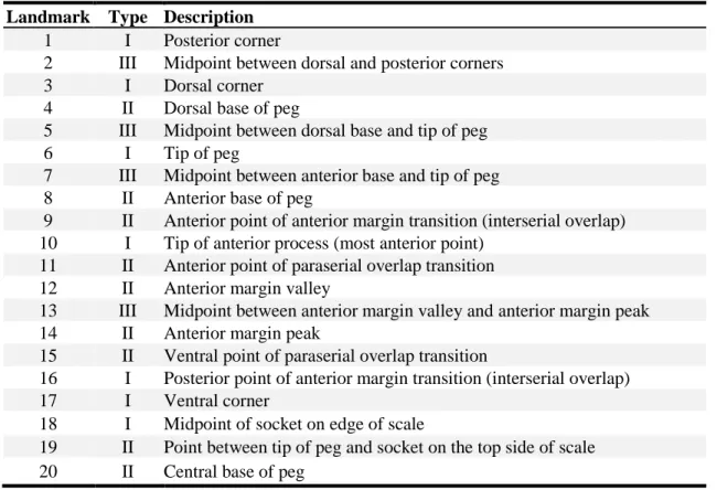
Table 2.1: Typology and descriptions for the 20 LMs defining the 2D scale geometry. ... 38 Table 2.2: 2D Morphometric parameters, descriptions, and calculations. ... 44 Table 2.3: P-values from student’s t-test of morphometric parameters of scales grouped by

region in the fish exoskeleton: average (N = 30 scales), anterior (N = 36 scales), tail (N = 21 scales), ventral (N = 41 scales), and pectoral fin (N = 14 scales). Asterisks (*) represent p-values < 0.01. ... 51 Table 3.1: Landmark typology and descriptions for the 21 LMs defining the 3D scale geometry.

... 60 Table 3.2: Parameters used in the 3D morphometric analysis, illustrated in Fig. 3.2. ... 62 Table 5.1: Displacement range, stiffness, and interscale mobility mechanisms for each loading

(23)

23

1. Introduction

1.1. Motivation

This thesis explores the use of shape and shape variation as a materials design parameter to control the mechanical behavior of materials in nature and in bioinspired analogs with the goal of developing flexible armor. Structural biological materials incorporate classical materials design parameters with morphometry (geometry or shape-based rules) to create

high-performance, multi-functional structures that exhibit tunable properties through extraordinary complexity, hierarchy, and precise structural control [1-8]. Geometric control of composite architectures can generate emergent material properties that outperform their base constituents such as high fracture toughness (e.g. in bone [9], nacre [10-12], and silica sponge skeletons [13]), extensive deformability (e.g. in skull sutures [14], wood cell walls [15], and shark cartilage [16]), actuation ability (e.g. in pine cones [17], seed capsules [18], and contractile roots [19]), or

functional transition regimes between different materials (e.g. bone-ligament junctions [20], bone porosity gradients [21], and mussel byssus [22]). Selective pressures have led many soft-bodied animals to evolve hard, protective exoskeletons as natural armors (e.g. crustaceans [23], insects [24], mollusks [25-26], turtles [27-28], sea horses [29], and bony fish [30-33]) with intricate, hierarchical microstructures that exhibit excellent strength, toughness, and energy dissipation mechanisms, while also using geometrical design rules to introduce an array of additional functionalities such as multi-scale enhancement of mechanical properties [25, 28, 33-35], transparency [36], or flexibility [26, 37]. Armored fish in particular have evolved protective exoskeletons that provide penetration resistance while maintaining flexibility through scale geometry, arrangement, and interlocking mechanisms [30-32, 37-38]. Research on biological and bioinspired structural materials has largely focused on the inherent materials-based structure-property relationships including hierarchy [2, 11], spatial heterogeneity [39], anisotropy [40], mechanical property amplification [2], and threat-specific deformation mechanisms [30, 32]. With advent of high resolution materials characterization instrumentation, powerful

computational simulation tools, and increasingly precise additive manufacturing techniques, it is becoming possible to study, replicate, and capitalize on the full range of hybrid

materials-morphometric design principles found in nature.

Bioinspired engineering that integrates both materials and morphometric design

principles shows promise for the development of flexible armor [38]. While the development of penetration resistant materials has progressed rapidly [41], there exists a tradeoff between protection and flexibility within current armor technology (Fig. 1.1). Today, large, monolithic plate armors are in use with various materials that are tailored to the application, such as metals like steel [42], ceramics like aluminum oxides, silicon carbides, and boron carbides [43], and Kevlar aramid fibers [44]. Flexibility can be introduced by segmenting plates into smaller units, such as in vest inserts [45] or elbow pads [46], leaving vulnerable weak spots in the gaps

(24)

24

between materials. Further attempts at engineering synthetic flexible armors have used simple geometries and assembly configurations [47-48], for example in mosaic tiled armor [49], articulating concrete mats [50], and flexible protective vests [51-52]. However, these designs tend to fail at the interfaces between materials, such as the adhesive attaching overlapping ceramic discs to the substrate in DragonSkin [52]. Using additive manufacturing as a fabrication method can eliminate the need for adhesives and mitigate interface failure while allowing for complex subunit shapes, multi-materiality, and tailorable material choice for target applications. Emerging biomimetic armors based on articulated fish armor designs can be useful for damage localization, flexibility, customizable design and fit, and selective replacement of damaged units.

Figure 1.1: The protection vs. flexibility tradeoff in current armor technologies [42-46, 52].

1.2. Overview

This thesis explores the use of morphometric-enabled materials design through the

development of bio-inspired, flexible composite armor based on the articulated exoskeleton of an armored fish, Polypterus senegalus, which possesses a protective ganoid squamation that

achieves uniform coverage and protection from predatory threats without restricting flexibility [53-55]. First, the functional implications of scale shape and shape variation are examined as materials design parameters within the biological exoskeleton using a new method that integrates continuum strain analysis with landmark-based geometric morphometric analysis in 2D

(Chapter 2) and 3D (Chapter 3). Bioinspired flexible composite prototypes are then fabricated using multi-material 3D printing and tested under passive loading under self-weight (Chapter 4) and active loading in bending (Chapter 5) to examine how the shape of scales contributes to local, interscale mobility mechanisms that generate anisotropic, global mechanical behavior. With one prototype design scheme, a wide array of mechanical behavior is generated with stiffness ranging over several orders of magnitude, thus showing how morphometry can tune the flexibility of composite architectures without varying the constituent materials. In the orientation that exhibits the greatest flexibility, the scales are considered ‘mechanically invisible’ and do not add stiffness to the armor assembly. Finite element models simulating the bending experiments

(25)

25

are then created to establish a computational framework for analyzing the mechanical response of the prototypes, and the models are extended to analyze behavior in other loading conditions, e.g. convex bending and tension (Chapter 6). The finite element simulations are further extended to examine the effect of the multi-material architecture, scale morphometry, and

constituent material properties on the mechanical response of the bio-inspired, flexible composite materials (Chapter 7). Finally, conclusions and future directions stemming from the work

presented in this thesis are discussed (Chapter 8). The results show how morphometric-enabled materials design, inspired by structural biological materials, can allow for tunable behavior in flexible composites made of segmented scale assemblies to achieve enhanced user mobility, custom fit, and flexibility around joints for a variety of protective applications.

1.3. Background

The model system used in this thesis is the armored fish, Polypterus senegalus (bichir), which possesses a mineralized, full-coverage exoskeleton, shown in Fig. 1.2a-b, with flexibility for axial bending and torsion [53-55], escape maneuvers [56], and recoil aspiration [57]. The exoskeleton uses a hierarchy of design rules to enable multifunctional behavior (Fig. 1.2); heterogeneity in material structure and properties provides protection, while morphometry and articulation mechanisms contribute to flexibility [30, 55, 58-62]. The evolution of P. senegalus armor, its material composition, geometric design rules explored to date, and preliminary work toward creating bioinspired flexible composite prototypes are described below.

1.3.1. Evolution of the biological model system: Polypterus senegalus

P. senegalus (phylum Chordata, superclass Osteichthyes (bony fish), class Actinopterygii (ray-finned fish), order Polpteriformes, family Polypteridae) originated in the Cretaceous period approximately 95 million years ago [53-54]. The species has an exoskeleton comprised of

armored, ganoid scales with a microstructure characteristic of ancient palaeoniscoid fish [63-64]. Dermal fish armor first appeared in Ostracoderms in the Paleozoic era approximately 500

million years ago [65] in response to predatory threats [66-67] with multilayered structures and geometries [68-69]. The large, heavy dermal armor plates broke into several smaller plates during the Devonian period (approximately 400 million years ago) as fish became predators and required faster swimming agility with light-weight armor and greater flexibility [66, 70]. The number of material layers in the armor decreased (from 4 to 1-3 layers), and the thickness of each material layer decreased (from 1500 to 100 µm thick) [53, 63]. Armored fish living today exhibit three major types of bony scales: ganoid, elasmoid, and placoid [54, 71]. While these categories of scales differ in shape, layered microstructure, and biomineralization processes, they are all made of the same mineral component, calcium phosphate, in the form of hydroxyapatite [72]. By contrast, many invertebrate exoskeletons, e.g. mollusks and sea urchins, are composed of calcium carbonate [73]. In the present day, P. senegalus lives in freshwater estuaries and shallow floodplains in Africa [74]. This species can be self-predatory [65], with a jaw structure and skull capable of powerful biting attacks during territorial fighting and feeding [74-77].

(26)

26

Figure 1.2: The hierarchical materials-morphometric design principles of the P. senegalus exoskeleton. (a) X-ray microcomputed tomography (µCT) reconstruction of a P. senegalus specimen, adapted from

[58]. (b) Anesthetized P. senegalus specimen (body length = 219 mm) exhibiting large bi-directional body curvature in axial bending [59]. (c) Optical micrographs of a single scale cross-section showing

(27)

27

the quad-layered structure [30, 60]. (d) Scanning electron micrograph (SEM) of ganoine nanocrystals [30]. (e) SEM of the dentin layer [61]. (f) Backscatter SEM (BSEM) of isopedine cross-section [60]. (g) Atomic force micrograph (AFM), height-image, of a polished cross section of the bony plate [61]. (h) Optical micrographs of 1N and 2N microindentations on scale surface showing circumferential cracking [30]. (i) BSEM showing crack arrest at the ganoine-dentin junction [30]. (j) Schematic of the helical arrangement of scales showing the paraserial axis (red) and interserial axis (black) [55]. (k) Schematic showing the local articulation of scales. (l) µCT reconstruction of a single scale, interior (left) and exterior (right) views [62]. (m) SEM of outer scale surface [30]. (n) SEM of inner scale surface [30]. (o) Schematic of the articulated, paraserial peg-and-socket joint [62]. (p) Schematic of the sliding,

interserial overlap joint [62]. (q) Schematic of the interior view of the local assembly of scales, showing sites of attachment of Sharpey’s fibers (asf) and attachment of stratum compactum (asc), as well as the fibers of the stratum compactum (sc) that run along the paraserial (ps) and interserial (is) axes [55]. (r) SEM of the interior of the scale showing the site of attachment of the stratum compactum to the axial ridge of the scale [55]. (s) SEM of stratum compactum [55]. (t) SEM showing Sharpey’s fibers connecting the peg and socket of adjacent scales [55].

1.3.2. Material composition of individual P. senegalus scales

The materiality of the mineralized ganoid scales underlies the protective functionality of the exoskeleton (Fig 1.2c-i). The ganoid scales have a quad-layered microstructure of

hydroxyapatite-organic composite materials, shown in Fig. 1.2c, composed of outermost ganoine (~10 µm thick, elastic modulus (E) = 55 GPa, >95% mineral content), dentin (~50 µm thick, E = 25 GPa, ~80% mineral content), isopedine (~40 µm thick, E = 14.5 GPa, 60-75% mineral

content), and innermost bone (~300 µm thick, E = 13.5 GPa, 60-70% mineral content) with a porous architecture [30, 32, 54, 60-61, 78-82]. Each layer has a unique nanocomposite structure [30, 61]. The thin, outer ganoine layer (Fig. 1.2d) is a stratified, acellular, and highly mineralized collection of pseudoprismatic apatite crystallites (50 nm diameter) that twist in bundles toward the outer scale surface [30]. Dentin (Fig. 1.2e) consists of 1-2 µm diameter dentinal tubules consisting of type I collagen fibrils reinforced with nanocrystalline apatite (20-300 nm size) [30]. Isopedine (Fig. 1.2f) consists of orthogonal, collagenous layers alternating in thickness (3 µm and 6 µm), arranged in a plywood structure, and mineralized with apatite platelets (40-150 nm) [30]. The bony basal plate (Fig. 1.2g), which forms the bulk of the scale, is composed of vascularized bone lamellae with collagen fibrils aligned parallel to the scale surface [30]. The materials are interpenetrated with each other at the layer interfaces; for instance, at the dentin-ganoine junction, dentin-ganoine nanorods penetrate into the dentin, and organic ligaments from dentin are anchored within the ganoine structure [30, 54].

The multilayered design enables penetration resistance, toughness, and non-catastrophic pathways for energy dissipation while exhibiting load-dependent material properties,

circumferential surface cracking, minimized weight, and microstructural length scale and material property length scale matching between the armor and the predatory teeth (threat matching) with optimized layer thickness [30, 32, 40, 83]. Each layer exhibits unique

deformation and energy dissipation mechanisms, and the functionally-graded junctions between layers promote load transfer and stress redistribution while preventing delamination [30]. The hardness and stiffness of the mineralized ganoine work in conjunction with the compliance of the

(28)

28

dentin layer to dissipate energy through plasticity at high loads, to reduce the weight of the scale by ~20% while maintaining protective functionality, and to promote localized, circumferential cracking while suppressing radial crack propagation (Fig. 1.2h) [30]. The stratification of isopedine arrests microcracks that penetrate deeply into the scale at high loads, preventing catastrophic failure of the scale (Fig. 1.2i) [30]. The material properties and thickness of each layer are optimized to defend against the animal’s primary threat, tooth-biting attacks, by both deforming and fracturing the threat (tooth) and by also allowing for non-catastrophic avenues for energy dissipation through deformation within the scale microstructure [32, 40].

1.3.3. Geometry and assembly of scales into the exoskeleton

The multilayered materials design of the individual scales works in conjunction with scale geometry and interlocking mechanisms to enable body flexibility [55]. The scales are articulated over the surface of the dermis to form a protective exoskeleton assembly (Fig. 1.2j-l), rather than imbricated into the soft tissue of the fish. The squamation consists of columns of scales that wind around the body in two interwoven, semi-helical axes depicted in Fig. 1.2j: the oblique paraserial axis of scale articulation and the interserial axis of scale overlap [55]. The local articulation of scales (Fig. 1.2k) is derived from the complex shape of the individual scale (Fig. 1.2l). Morphometric design rules guide scale articulation (Fig. 1.2m-p). The scales possess distinct geometric features, as shown in Fig. 1.2m-n, such as the peg, socket, anterior process, and axial ridge [30, 55]. These features create two joint interconnections between neighboring scales: the articulated peg-and-socket joint in the paraserial direction within a column of scales (Fig. 1.2o), and the sliding overlap joint in the interserial direction between columns of scales (Fig. 1.2p). The combination of both joints allows for complex relative motion in both axes, such as shear, splay, and double curvature [59].

Two fibrous systems provide interscale connectivity in the exoskeleton (Fig. 1.2q-t) [54-55, 84]. The peg-and-socket joint is reinforced, supported, and aligned by collagenous Sharpey’s fibers. The scales are connected to the underlying dermis through the stratum compactum, an organic, fibrous tissue extending from the axial ridge [55]. Fig. 1.2q shows the sites of

attachment of Sharpey’s fibers and attachment of stratum compactum on the interior of the scale assembly, as well as the fiber layers of the stratum compactum that run along the paraserial and interserial axes [55].

The shapes and sizes of scales vary throughout the fish exoskeleton, from large, heavily featured scales in the anterior region to small, featureless scales in the tail, yet the body

maintains small radii of axial body curvature throughout [55, 84]. The dorsal and ventral midlines, comprised of scales with specialized double-socketed or double-pegged geometries, respectively, represent axes of mirror symmetry in scale geometry and hold the paraserial

columns together [55]. Armored, limb-like pectoral fins extend from the main body exoskeleton. It has been shown that the ganoid integuments of bony, actinopterygian fish do not limit body flexibility compared to nonganoid integuments [55, 85], as was hypothesized in the past

(29)

29

[84, 86-88]. The complex shape, orientation, joint articulation, and assembly of scales in the exoskeleton do not limit the body curvature of P. senegalus during steady state undulatory motion and do not resist torsion, but rather guide bending of the fish in the horizontal plane [55]. In Polypterids and Lepisosteids, body curvature was found to be limited by the trunk

musculature in concave bending and strain on the stratum compactum in convex bending, rather than by the assembly of armored scales [55]. Experimentally, it was shown that cutting the dermis between scale rows in an armored Lepisosteid (Lepisosteus osseus, longnose gar) significantly reduces the flexural stiffness of the body, increases the neutral zone of curvature, and alters the swimming kinematics of the fish, whereas surgical removal of a scale row does not affect the body’s flexural stiffness [85].

1.3.4. Preliminary steps toward bio-inspired flexible armor

Prior research has made preliminary attempts at translating the components of the P. senegalus exoskeleton to synthetic prototypes to study the underlying kinematic schema. An individual scale was unitized, enlarged, and 3D printed with plaster to probe the scale geometry, morphology, and joint interconnections, shown in Fig. 1.3a [59-60]. Inclusion of material

heterogeneity in a single scale architecture demonstrated the potential for tailoring the individual scale units, shown in Fig. 1.3b [82]. Monolithic ring structures based on the P. senegalus

exoskeleton clarified the roles of the joints in axial bending and transverse stiffening of the exoskeleton (Fig. 1.3c) [59]. A simplified scale design was created to allow two rotational degrees of freedom at the paraserial and interserial joints (Fig. 1.3d) [59]. The simplified scale designs were fabricated by 3D printing and assembled with rubber bands to mimic the fibrous interconnections (Fig. 1.3e) [59]. Inclusion of compliant materials, e.g. the Sharpey’s fibers and stratum compactum in P. senegalus, within the prototype was achieved using multi-material 3D printing using TangoPlus (a soft, rubber-like elastomer) and VeroWhite (a hard, rigid polymer) on the Objet Connex 500 3D printer (Stratasys, USA). Small assemblies probing the local articulation of scales replicated the local scale-to-scale joint ranges of motion in the synthetic prototypes in Fig. 1.3f [59]. Arrays of large scales with a homogeneous geometry were printed in Fig. 1.3g [59]. However, a functional prototype that fully integrates both materials and

morphometric design rules has yet to be created, and the mechanical behavior of P. senegalus-inspired scale assemblies has yet to be analyzed.

(30)

30

Figure 1.3: Prior research in developing P. senegalus -inspired armor prototypes. (a) Two scales that

have been unitized, enlarged, and 3D printed with plaster [59]. (b) Single scale incorporating material heterogeneity through the scale’s porous architecture [82]. (c) Monolithic semi-helical ring structures [59]. (d) Simplified scale design allowing two rotational degrees of freedom at the paraserial and interserial joints [59]. (e) Simplified scale design from (d) 3D-printed and assembled with rubber bands to mimic the fibrous interconnections [59]. (f) 1×2 arrays of scales incorporating compliant material elements in the peg-and-socket interconnections (top) and the attachment site to the underlying substrate (bottom) using multimaterial 3D printing [59]. (g) 5×5 flexible scale assembly [59].

1.4. References

1. Arciszewski, T. & Cornell, J. in Bio-Inspiration: Learning Creative Design Principia (ed. Smith, I. F. C.) (Springer, Berlin, 2006).

2. Ortiz, C. & Boyce, M.C. Bioinspired Structural Materials. Science 319, 1053-1054 (2008).

3. Oyen, M. L., Bushby, A. J., Mann, A. & Ortiz, C. Mechanics of biological and biomimetic materials at small length scales. J. Mater. Res. 21, 1869-1870 (2006). 4. Wainwright, S. A., Biggs, W. D., Currey, J. D. & Gosline, J. M. Mechanical Design in

Organisms (Princeton Univ. Press, Princeton, 1976).

5. Chen, P. Y., McKittrick, J. & Meyers, M. A. Biological materials: functional adaptations and bioinspired designs. Prog. Mater. Sci. 57, 1492-1704 (2012).

6. Meyers, M. A., Chen, P. Y., Lin, A. Y. M. & Seki, Y. Biological materials: structure and mechanical properties. Prog. Mater. Sci. 53, 1-206 (2008).

7. Weiner, S. & Addadi, L. Design strategies in mineralized biological materials. J. Mater. Chem. 7, 689–702 (1997).

8. Dunlop, J.W.C., Weinkamer, R. & Fratzl, P. Artful interfaces within biological materials. Materials Today. 14, 70-78 (2011).

Biological and bio-inspired morphometry as a route to tunable and enhanced materials design

Biological and Bio-Inspired Morphometry as a Route

to Tunable and Enhanced Materials Design

by

Swati Varshney

BS Chemistry, Carnegie Mellon University (2010)

MPhil Micro- & Nanotechnology Enterprise, University of Cambridge (2011)

Biological and Bio-Inspired Morphometry as a Route

to Tunable and Enhanced Materials Design

by

Swati Varshney

Abstract

Acknowledgements

Table of Contents

L

F

...10

L

T

...22

1.

I

...23

2.

2D

M

H

S

P.

E

...36

3.

3D

M

H

S

P.

E

...58

4.

A

F

B

-

F

C

P

P

L

...73

5.

M

B

B

-I

F

C

P

A

L

...82

6.

F

E

S

B

-I

F

C

P

A

L

...92

7.

E

V

M

M

D

M