The MIT Faculty has made this article openly available.
Please share
how this access benefits you. Your story matters.
Citation
Ilya Baran and Jovan Popovic. 2007. Automatic rigging and
animation of 3D characters. ACM Trans. Graph. 26, 3, Article 72 (July
2007).
As Published
http://dx.doi.org/10.1145/1276377.1276467
Publisher
Association for Computing Machinery (ACM)
Version
Author's final manuscript
Citable link
http://hdl.handle.net/1721.1/100396
Terms of Use
Article is made available in accordance with the publisher's
policy and may be subject to US copyright law. Please refer to the
publisher's site for terms of use.
Automatic Rigging and Animation of 3D Characters
Ilya Baran∗ Jovan Popovi´c†
Computer Science and Artificial Intelligence Laboratory Massachusetts Institute of Technology
Abstract
Animating an articulated 3D character currently requires manual rigging to specify its internal skeletal structure and to define how the input motion deforms its surface. We present a method for ani-mating characters automatically. Given a static character mesh and a generic skeleton, our method adapts the skeleton to the character and attaches it to the surface, allowing skeletal motion data to an-imate the character. Because a single skeleton can be used with a wide range of characters, our method, in conjunction with a library of motions for a few skeletons, enables a user-friendly animation system for novices and children. Our prototype implementation, called Pinocchio, typically takes under a minute to rig a character on a modern midrange PC.
CR Categories: I.3.7 [Computer Graphics]: Three-Dimensional Graphics and Realism—Animation
Keywords: Animation, Deformations, Geometric Modeling
1
Introduction
Modeling in 3D is becoming much easier than before. User-friendly systems such as Teddy [Igarashi et al. 1999] and Cosmic Blobs (http://www.cosmicblobs.com/) have made the creation of 3D characters accessible to novices and children. Bringing these static shapes to life, however, is still not easy. In a conventional skeletal animation package, the user must rig the character man-ually. This requires placing the skeleton joints inside the charac-ter and specifying which parts of the surface are attached to which bone. The tedium of this process makes simple character animation more difficult than it could be.
We envision a system that eliminates this tedium to make an-imation more accessible for children, educators, researchers, and other non-expert animators. For example, a child should be able to model a unicorn, click the “Quadruped Gallop” button, and watch the unicorn start galloping. To support this functionality, we need a method (as shown in Figure 1) that takes a character, a skeleton, and a motion of that skeleton as input, and outputs the moving char-acter. The missing portion is the rigging: motion transfer has been addressed in prior work [Gleicher 2001].
Our algorithm consists of two main steps: skeleton embedding and skin attachment. Skeleton embedding computes the joint posi-tions of the skeleton inside the character by minimizing a penalty
∗e-mail: [email protected] †e-mail: [email protected]
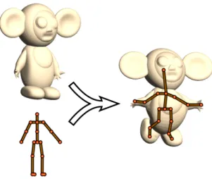
Figure 1: The automatic rigging method presented in this paper allowed us to implement an easy-to-use animation system, which we called Pinocchio. In this example, the triangle mesh of a jolly cartoon character is brought to life by embedding a skeleton inside it and applying a walking motion to the initially static shape.
function. To make the optimization problem computationally feasi-ble, we first embed the skeleton into a discretization of the charac-ter’s interior and then refine this embedding using continuous op-timization. The skin attachment is computed by assigning bone weights based on the proximity of the embedded bones smoothed by a diffusion equilibrium equation over the character’s surface.
Our design decisions relied on three criteria, which we also used to evaluate our system:
• Generality: A single skeleton is applicable to a wide vari-ety of characters: for example, our method can use a generic biped skeleton to rig an anatomically correct human model, an anthropomorphic robot, and even something that has very little resemblance to a human.
• Quality: The resulting animation quality is comparable to that of modern video games.
• Performance: The automatic rigging usually takes under one minute on an everyday PC.
A key design challenge is constructing a penalty function that pe-nalizes undesirable embeddings and generalizes well to new char-acters. For this, we designed a maximum-margin supervised learn-ing method to combine a set of hand-constructed penalty functions. To ensure an honest evaluation and avoid overfitting, we tested our algorithm on 16 characters that we did not see or use during devel-opment. Our algorithm computed a good rig for all but 3 of these characters. For each of the remaining cases, one joint placement hint corrected the problem.
We simplify the problem by making the following assumptions. The character mesh must be the boundary of a connected volume.
The character must be given in approximately the same orientation and pose as the skeleton. Lastly, the character must be proportioned roughly like the given skeleton.
We introduce several new techniques to solve the automatic rig-ging problem:
• A maximum-margin method for learning the weights of a lin-ear combination of penalty functions based on examples, as an alternative to hand-tuning (Section 3.3).
• An A∗-like heuristic to accelerate the search for an optimal
skeleton embedding over an exponential search space (Sec-tion 3.4).
• Use of Laplace’s diffusion equation to generate weights for at-taching mesh vertices to the skeleton using linear blend skin-ning (Section 4). This method could also be useful in existing 3D packages.
Our prototype system, called Pinocchio, rigs the given charac-ter using our algorithm. It then transfers a motion to the characcharac-ter using online motion retargetting [Choi and Ko 2000] to eliminate footskate by constraining the feet trajectories of the character to the feet trajectories of the given motion.
2
Related Work
Character Animation Most prior research in character anima-tion, especially in 3D, has focused on professional animators; very little work is targeted at novice users. Recent exceptions include Motion Doodles [Thorne et al. 2004] as well as the work of Igarashi et al. on spatial keyframing [2005b] and as-rigid-as-possible shape manipulation [2005a]. These approaches focus on simplifying an-imation control, rather than simplifying the definition of the artic-ulation of the character. In particular, a spatial keyframing system expects an articulated character as input, and as-rigid-as-possible shape manipulation, besides being 2D, relies on the constraints to provide articulation information. The Motion Doodles system has the ability to infer the articulation of a 2D character, but their ap-proach relies on very strong assumptions about how the character is presented.
Skeleton Extraction Although most skeleton-based prior work on automatic rigging focused on skeleton extraction, for our prob-lem, we advocate skeleton embedding. A few approaches to the skeleton extraction problem are representative. Teichmann and Teller [1998] extract a skeleton by simplifying the Voronoi skele-ton with a small amount of user assistance. Liu et al. [2003] use repulsive force fields to find a skeleton. In their paper, Katz and Tal [2003] describe a surface partitioning algorithm and suggest skele-ton extraction as an application. The technique in Wade [2000] is most similar to our own: like us, they approximate the medial sur-face by finding discontinuities in the distance field, but they use it to construct a skeleton tree.
For the purpose of automatically animating a character, however, skeleton embedding is much more suitable than extraction. For ex-ample, the user may have motion data for a quadruped skeleton, but for a complicated quadruped character, the extracted skeleton is likely to have a different topology. The anatomically appropriate skeleton generation by Wade [2000] ameliorates this problem by techniques such as identifying appendages and fitting appendage templates, but the overall topology of the resulting skeleton may still vary. For example, for the character in Figure 1, ears may be mistaken for arms. Another advantage of embedding over ex-traction is that the given skeleton provides information about the expected structure of the character, which may be difficult to ob-tain from just the geometry. So although we could use an existing skeleton extraction algorithm and embed our skeleton into the ex-tracted one, the results would likely be undesirable. For example,
the legs of the character in Figure 1 would be too short if a skeleton extraction algorithm were used.
Template Fitting Animating user-provided data by fitting a tem-plate has been successful in cases when the model is fairly similar to the template. Most of the work has been focused on human mod-els, making use of human anatomy specifics, e.g. [Moccozet et al. 2004]. For segmenting and animating simple 3D models of charac-ters and inanimate objects, Anderson et al. [2000] fit voxel-based volumetric templates to the data.
Skinning Almost any system for mesh deformation (whether sur-face based [Lipman et al. 2005; Yu et al. 2004] or volume based [Zhou et al. 2005]) can be adapted for skeleton-based deformation. Teichmann and Teller [1998] propose a spring-based method. Un-fortunately, at present, these methods are unsuitable for real-time animation of even moderate size meshes. Because of its simplicity and efficiency (and simple GPU implementation), and despite its quality shortcomings, linear blend skinning (LBS), also known as skeleton subspace deformation, remains the most popular method used in practice.
Most real-time skinning work, e.g. [Kry et al. 2002; Wang et al. 2007], has focused on improving on LBS by inferring the char-acter articulation from multiple example meshes. However, such techniques are unsuitable for our problem because we only have a single mesh. Instead, we must infer articulation by using the given skeleton as an encoding of the likely modes of deformation, not just as an animation control structure.
To our knowledge, the problem of finding bone weights for LBS from a single mesh and a skeleton has not been sufficiently ad-dressed in the literature. Previous methods are either mesh reso-lution dependent [Katz and Tal 2003] or the weights do not vary smoothly along the surface [Wade 2000], causing artifacts on high-resolution meshes. Some commercial packages use proprietary methods to assign default weights. For example, Autodesk Maya 7 assigns weights based solely on the vertex proximity to the bone, ignoring the mesh structure, which results in serious artifacts when the mesh intersects the Voronoi diagram faces between logically distant bones.
3
Skeleton Embedding
Skeleton embedding resizes and positions the given skeleton to fit inside the character. This can be formulated as an optimization problem: “compute the joint positions such that the resulting skele-ton fits inside the character as nicely as possible and looks like the given skeleton as much as possible.” For a skeleton withs joints (by “joints,” we mean vertices of the skeleton tree, including leaves), this is a3s-dimensional problem with a complicated objective func-tion. Solving such a problem directly using continuous optimiza-tion is infeasible.
Pinocchio therefore discretizes the problem by constructing a graph whose vertices represent potential joint positions and whose edges are potential bone segments. This is challenging because the graph must have few vertices and edges, and yet capture all poten-tial bone paths within the character. The graph is constructed by packing spheres centered on the approximate medial surface into the character and by connecting sphere centers with graph edges. Pinocchio then finds the optimal embedding of the skeleton into this graph with respect to a discrete penalty function. It uses the discrete solution as a starting point for continuous optimization.
To help with optimization, the given skeleton can have a lit-tle extra information in the form of joint attributes: for example, joints that should be approximately symmetric should be marked as such; also some joints can be marked as “feet,” indicating that they should be placed near the bottom of the character. We describe the attributes Pinocchio uses in a supplemental document[Baran and
Figure 2: Approximate Medial Sur-face
Figure 3: Packed Spheres Figure 4: Constructed Graph Figure 5: The original and reduced quadruped skeleton
Popovi´c 2007a]. These attributes are specific to the skeleton but are independent of the character shape and do not reduce the generality of the skeletons.
3.1 Discretization
Before any other computation, Pinocchio rescales the character to fit inside an axis-aligned unit cube. As a result, all of the tolerances are relative to the size of the character.
Distance Field To approximate the medial surface and to facili-tate other computations, Pinocchio computes a trilinearly interpo-lated adaptively sampled signed distance field on an octree [Frisken et al. 2000]. It constructs a kd-tree to evaluate the exact signed dis-tance to the surface from an arbitrary point. It then constructs the distance field from the top down, starting with a single octree cell and splitting a cell until the exact distance is within a toleranceτ of the interpolated distance. We found thatτ = 0.003 provides a good compromise between accuracy and efficiency for our purposes. Be-cause only negative distances (i.e. from points inside the character) are important, Pinocchio does not split cells that are guaranteed not to intersect the character’s interior.
Approximate Medial Surface Pinocchio uses the adaptive dis-tance field to compute a sample of points approximately on the medial surface (Figure 2). The medial surface is the set of C1
-discontinuities of the distance field. Within a single cell of our oc-tree, the interpolated distance field is guaranteed to beC1, so it is
necessary to look at only the cell boundaries. Pinocchio therefore traverses the octree and for each cell, looks at a grid (of spacing τ ) of points on each face of the cell. It then computes the gradient vectors for the cells adjacent to each grid point—if the angle be-tween two of them is120◦or greater, it adds the point to the medial
surface sample. We impose the120◦condition because we do not want the “noisy” parts of the medial surface—we want the points where skeleton joints are likely to lie. For the same reason, Pinoc-chio filters out the sampled points that are too close to the character surface (within2τ ). Wade discusses a similar condition in Chap-ter 4 of his thesis [2000].
Sphere Packing To pick out the graph vertices from the medial surface, Pinocchio packs spheres into the character as follows: it sorts the medial surface points by their distance to the surface (those that are farthest from the surface are first). Then it processes these points in order and if a point is outside all previously added spheres, adds the sphere centered at that point whose radius is the distance to the surface. In other words, the largest spheres are added first, and no sphere contains the center of another sphere (Figure 3). Although the procedure described above takesO(nb) time in the worst case (wheren is the number of points, and b is the final num-ber of spheres inserted), worst case behavior is rarely seen because most points are processed while there is a small number of large
spheres. In fact, this step typically takes less than1% of the time of the entire algorithm.
Graph Construction The final discretization step constructs the edges of the graph by connecting some pairs of sphere centers (Fig-ure 4). Pinocchio adds an edge between two sphere centers if the spheres intersect. We would also like to add edges between spheres that do not intersect if that edge is well inside the surface and if that edge is “essential.” For example, the neck and left shoulder spheres of the character in Figure 3 are disjoint, but there should still be an edge between them. The precise condition Pinocchio uses is that the distance from any point of the edge to the surface must be at least half of the radius of the smaller sphere, and the closest sphere centers to the midpoint of the edge must be the edge endpoints. The latter condition is equivalent to the requirement that additional edges must be in the Gabriel graph of the sphere centers (see e.g. [Jaromczyk and Toussaint 1992]). While other conditions can be formulated, we found that the Gabriel graph provides a good balance between sparsity and connectedness.
Pinocchio precomputes the shortest paths between all pairs of vertices in this graph to speed up penalty function evaluation. 3.2 Reduced Skeleton
The discretization stage constructs a geometric graphG = (V, E) into which Pinocchio needs to embed the given skeleton in an op-timal way. The skeleton is given as a rooted tree ons joints. To reduce the degrees of freedom, for the discrete embedding, Pinoc-chio works with a reduced skeleton, in which all bone chains have been merged (all degree two joints, such as knees, eliminated), as shown in Figure 5. The reduced skeleton thus has onlyr joints. This works because once Pinocchio knows where the endpoints of a bone chain are inV , it can compute the intermediate joints by taking the shortest path between the endpoints and splitting it in ac-cordance with the proportions of the unreduced skeleton. For the humanoid skeleton we use, for example,s = 18, but r = 7; with-out a reduced skeleton, the optimization problem would typically be intractable.
Therefore, the discrete skeleton embedding problem is to find the embedding of the reduced skeleton intoG, represented by an r-tuple v= (v1, . . . , vr) of vertices in V , which minimizes a penalty
functionf (v) that is designed to penalize differences in the embed-ded skeleton from the given skeleton.
3.3 Discrete Penalty Function
The discrete penalty function has great impact on the generality and quality of the results. A good embedding should have the propor-tions, bone orientapropor-tions, and size similar to the given skeleton. The paths representing the bone chains should be disjoint, if possible. Joints of the skeleton may be marked as “feet,” in which case they should be close to the bottom of the character. Designing a penalty function that satisfies all of these requirements simultaneously is
difficult. Instead we found it easier to design penalties indepen-dently and then rely on learning a proper weighting for a global penalty that combines each term.
The Setup We represent the penalty functionf as a linear com-bination ofk “basis” penalty functions: f (v) = Pk
i=1γibi(v).
Pinocchio usesk = 9 basis penalty functions constructed by hand. They penalize short bones, improper orientation between joints, length differences in bones marked symmetric, bone chains shar-ing vertices, feet away from the bottom, zero-length bone chains, improper orientation of bones, degree-one joints not embedded at extreme vertices, and joints far along bone-chains but close in the graph [Baran and Popovi´c 2007a]. We determine the weights Γ = (γ1, . . . , γk) semi-automatically via a new maximum margin
approach inspired by support vector machines.
Suppose that for a single character, we have several example em-beddings, each marked “good” or “bad”. The basis penalty func-tions assign a feature vector b(v) = (b1(v), . . . , bk(v)) to each
example embedding v. Let p1, . . . , pmbe thek-dimensional
fea-ture vectors of the good embeddings and let q1, . . . , qnbe the
fea-ture vectors of the bad embeddings.
Maximum Margin To provide context for our approach, we re-view the relevant ideas from the theory of support vector ma-chines. See Burges [1998] for a much more complete tuto-rial. If our goal were to automatically classify new embeddings into “good” and “bad” ones, we could use a support vector ma-chine to learn a maximum margin linear classifier. In its sim-plest form, a support vector machine finds the hyperplane that separates the pi’s from the qi’s and is as far away from them
as possible. More precisely, ifΓ is a k-dimensional vector with kΓk = 1, the classification margin of the best hyperplane normal to Γ is 1
2`min n
i=1ΓTqi− maxmi=1ΓTpi´. Recalling that the total
penalty of an embedding v isΓTb(v), we can think of the
maxi-mum marginΓ as the one that best distinguishes between the best “bad” embedding and the worst “good” embedding in the training set.
In our case, however, we do not need to classify embeddings, but rather find aΓ such that the embedding with the lowest penalty f (v) = ΓTb(v) is likely to be good. To this end, we want Γ to
distinguish between the best “bad” embedding and the best “good” embedding, as illustrated in Figure 6. We therefore wish to max-imize the optimization margin (subject tokΓk = 1), which we define as: n min i=1 Γ T qi− m min i=1 Γ T pi.
Because we have different characters in our training set, and be-cause the embedding quality is not necessarily comparable between different characters, we find theΓ that maximizes the minimum margin over all of the characters.
Our approach is similar to margin-based linear structured classi-fication [Taskar et al. 2003], the problem of learning a classifier that to each problem instance (cf. character) assigns the discrete label (cf. embedding) that minimizes the dot product of a weights vec-tor with basis functions of the problem instance and label. The key difference is that structured classification requires an explicit loss function (in our case, the knowledge of the quality of all possible skeleton embeddings for each character in the training set), whereas our approach only makes use of the loss function on the training la-bels and allows for the possibility of multiple correct lala-bels. This possibility of multiple correct skeleton embeddings prevented us from formulating our margin maximization problem as a convex optimization problem. However, multiple correct skeleton embed-dings are necessary for our problem in cases such as the hand joint being embedded into different fingers.
0 b1
Margin
Bad embeddings (qi’s):
BestΓ b2
Figure 6: Illustration of optimization margin: marked skeleton em-beddings in the space of their penalties (bi’s)
Learning Procedure The problem of finding the optimalΓ does not appear to be convex. However, an approximately optimalΓ is acceptable, and the search space dimension is sufficiently low (9 in our case) that it is feasible to use a continuous optimization method. We use the Nelder-Mead method [Nelder and Mead 1965] starting from randomΓ’s. We start with a cube [0, 1]k
, pick random normalizedΓ’s, and run Nelder-Mead from each of them. We then take the bestΓ, use a slightly smaller cube around it, and repeat.
To create our training set of embeddings, we pick a training set of characters, manually chooseΓ, and use it to construct skeleton embeddings of the characters. For every character with a bad em-bedding, we manually tweakΓ until a good embedding is produced. We then find the maximum marginΓ as described above and use this newΓ to construct new skeleton embeddings. We manually classify the embeddings that we have not previously seen, augment our training set with them, and repeat the process. IfΓ eventually stops changing, as happened on our training set, we use the found Γ. It is also possible that a positive margin Γ cannot be found, in-dicating that the chosen basis functions are probably inadequate for finding good embeddings for all characters in the training set.
For training, we used 62 different characters (Cosmic Blobs models, free models from the web, scanned models, and Teddy models), andΓ was stable with about 400 embeddings. The weights we learned resulted in good embeddings for all of the characters in our training set; we could not accomplish this by manually tuning the weights. Examining the optimization results and the extremal embeddings also helped us design better basis penalty functions.
Although this process of finding the weights is labor-intensive, it only needs to be done once. According to our tests, if the basis functions are carefully chosen, the overall penalty function gener-alizes well to both new characters and new skeletons. Therefore, a novice user will be able to use the system, and more advanced users will be able to design new skeletons without having to learn new weights.
3.4 Discrete Embedding
Computing a discrete embedding that minimizes a general penalty function is intractable because there are exponentially many em-beddings. However, if it is easy to estimate a good lower bound on f from a partial embedding (of the first few joints), it is possible to use a branch-and-bound method. Pinocchio uses this idea: it main-tains a priority queue of partial embeddings ordered by their lower bound estimates. At every step, it takes the best partial embedding from the queue, extends it in all possible ways with the next joint, and pushes the results back on the queue. The first full embedding extracted is guaranteed to be the optimal one. This is essentially the A* algorithm on the tree of possible embeddings. To speed up
the process and conserve memory, if a partial embedding has a very high lower bound, it is rejected immediately and not inserted into the queue.
Although this algorithm is still worst-case exponential, it is fast on most real problems with the skeletons we tested. We considered adapting an approximate graph matching algorithm, like [Gold and Rangarajan 1996], which would work much faster and enable more complicated reduced skeletons. However, computing the exact op-timum simplified penalty function design and debugging.
The joints of the skeleton are given in order, which induces an order on the joints of the reduced skeleton. Referring to the joints by their indices (starting with the root at index1), we define the parent functionpR on the reduced skeleton, such thatpR(i) (for
1 < i ≤ r) is the index of the parent of joint i. We require that the order in which the joints are given respects the parent relationship, i.e.pR(i) < i.
Our penalty function (f ) can be expressed as the sum of inde-pendent functions of bone chain endpoints (fi’s) and a term (fD)
that incorporates the dependence between different joint positions. The dependence between joints that have not been embedded can be ignored to obtain a lower bound onf . More precisely, f can be written as: f (v1, . . . , vr) = r X i=2 fi(vi, vpR(i)) + r X i=2 fD(v1, . . . , vi).
A lower bound when the firstk joints are embedded is then:
k X i=2 fi(vi, vpR(i)) + k X i=2 fD(v1, . . . , vi) + + X {i>k|pR(i)≤k} min vi∈V fi(vi, vpR(i))
IffDis small compared to thefi’s, as is often the case for us, the
lower bound is close to the true value off .
Because of this lower bound estimate, the order in which joints are embedded is very important to the performance of the optimiza-tion algorithm. High degree joints should be embedded first be-cause they result in more terms in the rightmost sum of the lower bound, leading to a more accurate lower bound. For example, our biped skeleton has only two joints of degree greater than two, so after Pinocchio has embedded them, the lower bound estimate in-cludesfiterms for all of the bone chains.
Because there is no perfect penalty function, discrete embedding will occasionally produce undesirable results (see Model 13 in Fig-ure 9). In such cases it is possible for the user to provide manual hints in the form of constraints for reduced skeleton joints. For ex-ample, such a hint might be that the left hand of the skeleton should be embedded at a particular vertex inG (or at one of several ver-tices). Embeddings that do not satisfy the constraints are simply not considered by the algorithm.
3.5 Embedding Refinement
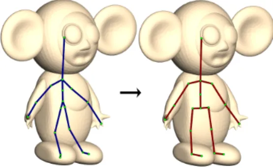
Pinocchio takes the optimal embedding of the reduced skeleton found by discrete optimization and reinserts the degree-two joints by splitting the shortest paths inG in proportion to the given skele-ton. The resulting skeleton embedding should have the general shape we are looking for, but typically, it will not fit nicely inside the character. Also, smaller bones are likely to be incorrectly ori-ented because they were not important enough to influence the dis-crete optimization. Embedding refinement corrects these problems by minimizing a new continuous penalty function (Figure 7).
For the continuous optimization, we represent the embedding of the skeleton as ans-tuple of joint positions (q1, . . . , qs) in R3.
Be-cause we are dealing with an unreduced skeleton, and discrete op-timization has already found the correct general shape, the penalty
Figure 7: The embedded skeleton after discrete embedding (blue) and the results of embedding refinement (dark red)
function can be much simpler than the discrete penalty function. The continuous penalty functiong that Pinocchio tries to minimize is the sum of penalty functions over the bones plus an asymmetry penalty: g(q1, . . . , qs) = αAgA(q1, . . . , qs) + s X i=2 gi(qi, qpS(i))
wherepS is the parent function for the unreduced skeleton
(anal-ogous topR). Eachgipenalizes bones that do not fit inside the
surface nicely, bones that are too short, and bones that are oriented differently from the given skeleton:gi= αSgiS+ αLgiL+ αOgiO.
Unlike the discrete case, we choose theα’s by hand because there are only four of them [Baran and Popovi´c 2007a].
Any continuous optimization technique [Gill et al. 1989] should produce good results. Pinocchio uses a gradient descent method that takes advantage of the fact that there are relatively few inter-actions. As a subroutine, it uses a step-doubling line search: start-ing from a given point (in R3s), it takes steps in the given opti-mization direction, doubling step length until the penalty function increases. Pinocchio intersperses a line search in the gradient di-rection with line searches in the gradient didi-rection projected onto individual bones. Repeating the process 10 times is usually suffi-cient for convergence.
4
Skin Attachment
The character and the embedded skeleton are disconnected until skin attachment specifies how to apply deformations of the skeleton to the character mesh. Although we could make use of one of the various mesh editing techniques for the actual mesh deformation, we choose to focus on the standard linear blend skinning (LBS) method because of its widespread use. If vjis the position of vertex
j, Ti
is the transformation of theithbone, andwi
jis the weight of
theithbone for vertexj, LBS gives the position of the transformed
vertexj asP
iw i
jTi(vj). The attachment problem is finding bone
weights wifor the vertices—how much each bone transform affects each vertex.
There are several properties we desire of the weights. First of all, they should not depend on the mesh resolution. Second, for the results to look good, the weights need to vary smoothly along the surface. Finally, to avoid folding artifacts, the width of a transi-tion between two bones meeting at a joint should be roughly pro-portional to the distance from the joint to the surface. Although a scheme that assigns bone weights purely based on proximity to bones can be made to satisfy these properties, such schemes will often fail because they ignore the character’s geometry: for exam-ple, part of the torso may become attached to an arm. Instead, we use the analogy to heat equilibrium to find the weights. Suppose we
Figure 8: Top: heat equilibrium for two bones. Bottom: the result of rotating the right bone with the heat-based attachment
treat the character volume as an insulated heat-conducting body and force the temperature of bonei to be 1 while keeping the tempera-ture of all of the other bones at0. Then we can take the equilibrium temperature at each vertex on the surface as the weight of bonei at that vertex. Figure 8 illustrates this in two dimensions.
Solving for heat equilibrium over a volume would require tes-sellating the volume and would be slow. Therefore, for simplic-ity, Pinocchio solves for equilibrium over the surface only, but at some vertices, it adds the heat transferred from the nearest bone. The equilibrium over the surface for bone i is given by ∂wi
∂t =
∆wi+ H(pi− wi) = 0, which can be written as
−∆wi+ Hwi= Hpi, (1) where ∆ is the discrete surface Laplacian, calculated with the cotangent formula [Meyer et al. 2003], piis a vector withpi
j = 1
if the nearest bone to vertexj is i and pi
j = 0 otherwise, and H is
the diagonal matrix withHjjbeing the heat contribution weight of
the nearest bone to vertexj. Because ∆ has units of length−2, so
must H. Lettingd(j) be the distance from vertex j to the nearest bone, Pinocchio usesHjj = c/d(j)2 if the shortest line segment
from the vertex to the bone is contained in the character volume andHjj = 0 if it is not. It uses the precomputed distance field to
determine whether a line segment is entirely contained in the char-acter volume. Forc ≈ 0.22, this method gives weights with similar transitions to those computed by finding the equilibrium over the volume. Pinocchio usesc = 1 (corresponding to anisotropic heat diffusion) because the results look more natural. Whenk bones are equidistant from vertexj, heat contributions from all of them are used:pjis1/k for all of them, and Hjj= kc/d(j)2.
Equation (1) is a sparse linear system, and the left hand side matrix−∆ + H does not depend on i, the bone we are interested in. Thus we can factor the system once and back-substitute to find the weights for each bone. Botsch et al. [2005] show how to use a sparse Cholesky solver to compute the factorization for this kind of system. Pinocchio uses the TAUCS [Toledo 2003] library for this computation. Note also that the weights wisum to 1 for each vertex: if we sum (1) overi, we get (−∆ + H)P
iw
i= H · 1,
which yieldsP
iw i= 1.
It is possible to speed up this method slightly by finding vertices that are unambiguously attached to a single bone and forcing their weight to 1. An earlier variant of our algorithm did this, but the im-provement was negligible, and this introduced occasional artifacts.
5
Results
We evaluate Pinocchio with respect to the three criteria stated in the introduction: generality, quality, and performance. To ensure an objective evaluation, we use inputs that were not used during development. To this end, once the development was complete, we tested Pinocchio on 16 biped Cosmic Blobs models that we had not previously tried.
Figure 10: A centaur pirate with a centaur skeleton embedded looks at a cat with a quadruped skeleton embedded
Figure 11: The human scan on the left is rigged by Pinocchio and is posed on the right by changing joint angles in the embedded skele-ton. The well-known deficiencies of LBS can be seen in the right knee and hip areas.
5.1 Generality
Figure 9 shows our 16 test characters and the skeletons Pinocchio embedded. The skeleton was correctly embedded into 13 of these models (81% success). For Models 7, 10 and 13, a hint for a single joint was sufficient to produce a good embedding.
These tests demonstrate the range of proportions that our method can tolerate: we have a well-proportioned human (Models 1–4, 8), large arms and tiny legs (6; in 10, this causes problems), and large legs and small arms (15; in 13, the small arms cause problems). For other characters we tested, skeletons were almost always correctly embedded into well-proportioned characters whose pose matched the given skeleton. Pinocchio was even able to transfer a biped walk onto a human hand, a cat on its hind legs, and a donut.
The most common issues we ran into on other characters were: • The thinnest limb into which we may hope to embed a bone
has a radius of2τ . Characters with extremely thin limbs often fail because the the graph we extract is disconnected. Reduc-ingτ , however, hurts performance.
• Degree 2 joints such as knees and elbows are often positioned incorrectly within a limb. We do not know of a reliable way to identify the right locations for them: on some characters they are thicker than the rest of the limb, and on others they are thinner.
Although most of our tests were done with the biped skeleton, we have also used other skeletons for other characters (Figure 10). 5.2 Quality
Figure 11 shows the results of manually posing a human scan us-ing our attachment. Our video [Baran and Popovi´c 2007b] demon-strates the quality of the animation produced by Pinocchio.
1. 2. 3. 4. 5. 6.
7. 8. 9. 10. 11. 12.
13. 14. 15. 16.
Figure 9: Test Results for Skeleton Embedding
Model 3 10 11 Mean Number of Vertices 19,001 34,339 56,856 33,224 Discretization Time 10.3s 25.8s 68.2s 24.3s Embedding Time 1.4s 29.1s 5.7s 5.2s Attachment Time 0.9s 1.9s 3.2s 1.8s Total Time 12.6s 56.8s 77.1s 31.3s Table 1: Timings for three representative models and the mean over our 16 character test set
The quality problems of our attachment are a combination of the deficiencies of our automated weights generation as well as those inherent in LBS. A common class of problems is caused by Pinoc-chio being oblivious to the material out of which the character is made: the animation of both a dress and a knight’s armor has an unrealistic, rubbery quality. Other problems occur at difficult ar-eas, such as hips and the shoulder/neck region, where hand-tuned weights could be made superior to those found by our algorithm. 5.3 Performance
Table 1 shows the fastest and slowest timings of Pinocchio rigging the 16 models discussed in Section 5.1 on a 1.73 MHz Intel Core Duo with 1GB of RAM. Pinocchio is single-threaded so only one core was used. We did not run timing tests on denser models be-cause someone wishing to create real-time animation is likely to keep the triangle count low. Also, because of our volume-based ap-proach, once the distance field has been computed, subsequent dis-cretization and embedding steps do not depend on the given mesh size.
For the majority of models, the running time is dominated by the discretization stage, and that is dominated by computing the distance field. Embedding refinement takes about 1.2 seconds for all of these models, and the discrete optimization consumes the rest of the embedding time.
6
Conclusion and Future Work
We have presented the first method for automatically rigging an unfamiliar character for skeletal animation. In conjunction with
ex-isting techniques, it allows a user to go from a static mesh to an animated character quickly and effortlessly. We have shown that using this method, Pinocchio can animate a wide range of charac-ters. We also believe that some of our techniques, such as finding LBS weights and using examples to learn the weights of a linear combination of penalty functions, can be useful in other contexts.
We have several ideas for improving Pinocchio that we have not yet tried. Discretization could be improved by packing ellipsoids instead of spheres. Although this is more difficult, we believe it would greatly reduce the size of the graph, resulting in faster and higher quality discrete embeddings. Animation quality can be im-proved with a better skinning model [Kavan and ˇZ´ara 2005] (al-though possibly at the cost of performance). One approach would be to use a technique [Wang et al. 2007] that corrects LBS errors by using example meshes, which we could synthesize using slower, but more accurate deformation techniques. A more involved approach would be automatically building a tetrahedral mesh around the em-bedded skeleton and applying the dynamic deformation method of Capell et al. [2002]. Combining retargetting with joint limits should eliminate some artifacts in the motion. A better retargetting scheme could be used to make animations more physically plausible and prevent global self-intersections. Finally, it would be nice to elim-inate the assumption that the character must have a well-defined interior.
Beyond Pinocchio’s current capabilities, an interesting problem is dealing with hand animation to give animated characters the abil-ity to grasp objects, type, or speak sign language. The variety of types of hands makes this challenging (see, for example, Models 13, 5, 14, and 11 in Figure 9). Automatically rigging characters for fa-cial animation is even more difficult, but a solution requiring a small amount of user assistance may succeed. Combined with a system for motion synthesis [Arikan et al. 2003], this would allow users to begin interacting with their creations.
7
Acknowledgments
We thank Yeuhi Abe and Eugene Hsu for help with motion cap-ture. Thanks to Soonmin Bae, Inna Baran, Fr´edo Durand, Sylvain Paris, Ariel Shamir, Daniel Vlasic, and Robert Wang for their help-ful feedback. Thanks to Emily Whiting for narrating the video. We
thank Dragomir Anguelov for the human meshes. We would also like to thank Solidworks for the permission to use Cosmic Blobs models. This work was supported by a grant from Solidworks Cor-poration. The first author was also supported by an NSF Graduate Research Fellowship.
References
ANDERSON, D., FRANKEL, J. L., MARKS, J., AGARWALA, A., BEARDSLEY, P., HODGINS, J., LEIGH, D., RYALL, K., SUL
-LIVAN, E.,ANDYEDIDIA, J. S. 2000. Tangible interaction + graphical interpretation: a new approach to 3d modeling. In Pro-ceedings of ACM SIGGRAPH 2000, Annual Conference Series, 393–402.
ARIKAN, O., FORSYTH, D. A.,ANDO’BRIEN, J. F. 2003. Mo-tion synthesis from annotaMo-tions. ACM TransacMo-tions on Graphics 22, 3 (July), 402–408.
BARAN, I., AND POPOVIC´, J., 2007. Penalty func-tions for automatic rigging and animation of 3d characters. http://people.csail.mit.edu/ibaran/penalty.pdf.
BARAN, I., AND POPOVIC´, J., 2007. Pinocchio results video. http://people.csail.mit.edu/ibaran/pinocchio.avi.
BOTSCH, M., BOMMES, D.,ANDKOBBELT, L. 2005. Efficient linear system solvers for mesh processing. In IMA Conference on the Mathematics of Surfaces, 62–83.
BURGES, C. 1998. A Tutorial on Support Vector Machines for Pattern Recognition. Data Mining and Knowledge Discovery 2, 2, 121–167.
CAPELL, S., GREEN, S., CURLESS, B., DUCHAMP, T., AND
POPOVIC´, Z. 2002. Interactive skeleton-driven dynamic defor-mation. ACM Transactions on Graphics 21, 3 (Aug.), 586–593. CHOI, K.-J., ANDKO, H.-S. 2000. Online motion retargetting. Journal of Visualization and Computer Animation 11, 5 (Dec.), 223–235.
FRISKEN, S. F., PERRY, R. N., ROCKWOOD, A. P.,ANDJONES, T. R. 2000. Adaptively sampled distance fields: A general rep-resentation of shape for computer graphics. In Proceedings of ACM SIGGRAPH 2000, Annual Conference Series, 249–254. GILL, P. E., MURRAY, W.,ANDWRIGHT, M. H. 1989. Practical
Optimization. Academic Press, London.
GLEICHER, M. 2001. Comparing contraint-based motion editing methods. Graphical Models 63 (Aug.), 107–134.
GOLD, S.,ANDRANGARAJAN, A. 1996. A graduated assignment algorithm for graph matching. IEEE Transactions on Pattern Analysis and Machine Intelligence 18, 4, 377–388.
IGARASHI, T., MATSUOKA, S.,ANDTANAKA, H. 1999. Teddy: A sketching interface for 3d freeform design. In Proceedings of ACM SIGGRAPH 1999, Annual Conference Series, 409–416. IGARASHI, T., MOSCOVICH, T., AND HUGHES, J. F. 2005.
As-rigid-as-possible shape manipulation. ACM Transactions on Graphics 24, 3 (Aug.), 1134–1141.
IGARASHI, T., MOSCOVICH, T.,ANDHUGHES, J. F. 2005. Spa-tial keyframing for performance-driven animation. In Sympo-sium on Computer Animation (SCA), 107–115.
JAROMCZYK, J. W., ANDTOUSSAINT, G. T. 1992. Relative neighborhood graphs and their relatives. Proceedings of IEEE 80, 9 (Sept.), 1502–1517.
KATZ, S.,ANDTAL, A. 2003. Hierarchical mesh decomposition using fuzzy clustering and cuts. ACM Transactions on Graphics 22, 3 (Aug.), 954–961.
KAVAN, L.,ANDZ ´ˇARA, J. 2005. Spherical blend skinning: A real-time deformation of articulated models. In ACM SIGGRAPH Symposium on Interactive 3D Graphics and Games, 9–16. KRY, P. G., JAMES, D. L., ANDPAI, D. K. 2002. EigenSkin:
Real time large deformation character skinning in hardware. In Symposium on Computer Animation (SCA), 153–160.
LIPMAN, Y., SORKINE, O., LEVIN, D., AND COHEN-OR, D. 2005. Linear rotation-invariant coordinates for meshes. ACM Transactions on Graphics 24, 3 (Aug.), 479–487.
LIU, P.-C., WU, F.-C., MA, W.-C., LIANG, R.-H.,ANDOUHY
-OUNG, M. 2003. Automatic animation skeleton using repulsive force field. In 11th Pacific Conference on Computer Graphics and Applications, 409–413.
MEYER, M., DESBRUN, M., SCHRODER¨ , P.,ANDBARR, A. H. 2003. Discrete differential-geometry operators for triangulated 2-manifolds. In Visualization and Mathematics III. Springer-Verlag, Heidelberg, 35–57.
MOCCOZET, L., DELLAS, F., MAGNENAT-THALMANN, N., BI
-ASOTTI, S., MORTARA, M., FALCIDIENO, B., MIN, P.,AND
VELTKAMP, R. 2004. Animatable human body model recon-struction from 3d scan data using templates. In CapTech Work-shop on Modelling and Motion Capture Techniques for Virtual Environments, 73–79.
NELDER, J.,ANDMEAD, R. 1965. A simplex method for function minimization. Computer Journal 7, 308–313.
TASKAR, B., GUESTRIN, C., AND KOLLER, D. 2003. Max-margin markov networks. In Advances in Neural Information Processing Systems (NIPS 2003).
TEICHMANN, M.,ANDTELLER, S. 1998. Assisted articulation of closed polygonal models. In Computer Animation and Simula-tion ’98, 87–102.
THORNE, M., BURKE, D.,AND VAN DEPANNE, M. 2004. Mo-tion doodles: an interface for sketching character moMo-tion. ACM Transactions on Graphics 23, 3 (Aug.), 424–431.
TOLEDO, S., 2003. TAUCS: A library of sparse linear solvers, version 2.2. http://www.tau.ac.il/∼stoledo/taucs.
WADE, L. 2000. Automated generation of control skeletons for use in animation. PhD thesis, The Ohio State University.
WANG, R., PULLI, K., AND POPOVIC´, J. 2007. Real-time enveloping with rotational regression. ACM Transactions on Graphics 26, 3. In press.
YU, Y., ZHOU, K., XU, D., SHI, X., BAO, H., GUO, B.,AND
SHUM, H.-Y. 2004. Mesh editing with poisson-based gradient field manipulation. ACM Transactions on Graphics 23, 3 (Aug.), 644–651.
ZHOU, K., HUANG, J., SNYDER, J., LIU, X., BAO, H., GUO, B.,
ANDSHUM, H.-Y. 2005. Large mesh deformation using the volumetric graph laplacian. ACM Transactions on Graphics 24, 3 (Aug.), 496–503.