Publisher’s version / Version de l'éditeur:
Vous avez des questions? Nous pouvons vous aider. Pour communiquer directement avec un auteur, consultez la première page de la revue dans laquelle son article a été publié afin de trouver ses coordonnées. Si vous n’arrivez pas à les repérer, communiquez avec nous à [email protected].
Questions? Contact the NRC Publications Archive team at
[email protected]. If you wish to email the authors directly, please see the first page of the publication for their contact information.
https://publications-cnrc.canada.ca/fra/droits
L’accès à ce site Web et l’utilisation de son contenu sont assujettis aux conditions présentées dans le site
LISEZ CES CONDITIONS ATTENTIVEMENT AVANT D’UTILISER CE SITE WEB.
Student Report; no. SR-2010-10, 2010-04-01
READ THESE TERMS AND CONDITIONS CAREFULLY BEFORE USING THIS WEBSITE. https://nrc-publications.canada.ca/eng/copyright
NRC Publications Archive Record / Notice des Archives des publications du CNRC :
https://nrc-publications.canada.ca/eng/view/object/?id=5bba65bf-b8d8-4894-a81b-d3fde86491dd https://publications-cnrc.canada.ca/fra/voir/objet/?id=5bba65bf-b8d8-4894-a81b-d3fde86491dd
NRC Publications Archive
Archives des publications du CNRC
For the publisher’s version, please access the DOI link below./ Pour consulter la version de l’éditeur, utilisez le lien DOI ci-dessous.
https://doi.org/10.4224/17618859
Access and use of this website and the material on it are subject to the Terms and Conditions set forth at
Procedure for Podded Propulsion Simulation
DOCUMENTATION PAGE
REPORT NUMBER SR-2010-10
NRC REPORTNUMBER DATE April 2010 REPORT SECURITY CLASSIFICATION
Unclassified
DISTRIBUTION Unlimited TITLE
PROCEDURE FOR PODDED PROPULSION SIMULATION AUTHOR(S)
Potchara Wongyai and Michael Lau CORPORATE AUTHOR(S)/PERFORMING AGENCY(S)
Institute for Ocean Technology, National Research Council, St. John’s, NL
PUBLICATION
SPONSORING AGENCY(S)
Transport Canada and Centre for Marine Simulation, Marine Institute IOT PROJECT NUMBER
2409
NRC FILENUMBER
KEY WORDS
pod, simulation, procedure, Polaris, OSIS
PAGES v, 28 FIGS. 20 TABLES 3 SUMMARY
A procedure for podded propulsion simulation using IOT OSIS and Kongsberg Polaris software simulators was developed based on the Mackinaw model test in open water. The data to be simulated in OSIS and Polaris is prepared from the data of static and dynamic model testing. The process to prepare the data involved determining the data that would be appropriate for a certain simulation and preparing the data into the right format. This involved the use of the IOT analysis software SWEET for file conversion and the Pod Analysis program developed prior to the project. The data was then applied to the Data Management program to adjust and modified the data before transferring to OSIS and the Polaris database generator. To ensure the accuracy for both simulators, the results of Mackinaw simulation in OSIS and Polaris were compared. Additional instruction on the Data Management program is also provided.
ADDRESS National Research Council Institute for Ocean Technology Arctic Avenue, P. O. Box 12093 St. John's, NL A1B 3T5
National Research Council Conseil national de recherches Canada Canada Institute for Ocean Institut des technologies Technology océaniques
PROCEDURE FOR PODDED PROPULSION SIMULATION
SR-2010-10Potchara Wongyai and Michael Lau
ACKNOWLEDGEMENTS
This work was supported by Transport Canada. Its financial support is gratefully acknowledged. The procedure for pod simulation based on Mackinaw model test was developed with great contribution and supervision from Dr. Michael Lau of IOT. Technical knowledge and programming technique was greatly supported by Dr. Shaoyu Ni, and suggestion about analysis of pod data and knowledge about model testing were given by Dr. Ayhan Akinturk of IOT. Ms. Renee Boileau of IOT
ABSTRACT
A procedure for podded propulsion simulation using IOT OSIS and Kongsberg Polaris software simulators was developed based on the Mackinaw model test in open water. The data to be simulated in OSIS and Polaris is prepared from the data of static and dynamic model testing. The process to prepare the data involved
determining the data that would be appropriate for a certain simulation and preparing the data into the right format. This involved the use of the IOT analysis software SWEET for file conversion and the Pod Analysis program developed prior to the project. The data was then applied to the Data Management program to adjust and modified the data before transferring to OSIS and the Polaris database generator. To ensure the accuracy for both simulators, the results of Mackinaw simulation in OSIS and Polaris were compared. Additional instruction on the Data Management program is also provided.
TABLE OF CONTENTS
ACKNOWLEDGEMENTS ... III ABSTRACT ... IV
1 INTRODUCTION ... 1
2 TESTING SCHEMES AND ASSUMPTIONS ... 2
3 PROCEDURE FOR SIMULATION ... 6
3.1 Acquiring Data from Model Test and Choosing Runs for the Simulation ... 7
3.2 Conversion from .DAC file... 8
3.3 Preparation for static and dynamic test data ... 11
3.4 OSIS simulation for Mackinaw ... 14
3.5 Generating database for Polaris ... 21
3.6 Based Calculation for Data Modification with Data Management program 21 3.7 Verification of Results ... 24
4 CONCLUSION AND RECOMMENDATION... 27
LIST OF FIGURES
Figure 2.1: Rudder angle and azimuthing angle convention... 3
Figure 2.2: Unparallel flow with Drift Angle... 4
Figure 3.1: Overall process for Mackinaw pod propulsion simulation ... 6
Figure 3.2: A template for the conversion of .DAC file to .CSV file ... 8
Figure 3.3: Segment selector for static run... 9
Figure 3.4: Segment selector for dynamic run... 10
Figure 3.5 Loading file name for the Podded Analysis program ... 12
Figure 3.6: Output graph from Podded Analysis program ... 13
Figure 3.7 pod_option in “Mackinaw55InIceNew.ocs” ... 15
Figure 3.8: Input data screen ... 16
Figure 3.9: Display screen showing the data of Kq,KFx, and KFy ... 17
Figure 3.10: Data editing screen ... 18
Figure 3.11: Data Extension screen for inputting dynamic test data... 19
Figure 3.12: Complete data for Kq... 20
Figure 3.13: Complete data for KFx... 20
Figure 3.14: Complete data for KFy... 21
Figure 3.15: Example trend-line of Kqversus J for Run 97 ... 22
Figure 3.16: Surface representation of Kqas a function of J and ... 23
Figure 3.18: Example for KFx graph with the extended data ... 24
Figure 3.19: Diameter Comparison between OSIS and Polaris... 25
Figure 3.20: Ship speed comparison between OSIS and Polaris ... 26
LIST OF TABLES Table 3.1: Static and dynamic run in Mackinaw simulation ... 7
Table 3.2: Static input file format ... 11
PROCEDURE FOR PODDED PROPULSION SIMULATION 1 INTRODUCTION
Podded propulsion simulation is an imitation of podded propulsor behavior of a real ship under various assumptions to predict the character and performance of the propulsion module of the ship. Podded propulsion simulation in this project focuses on determining propulsive forces and shaft power of the podded propellers of the U.S. Coast Guard icebreaker Mackinaw, in which the analysis was based on a model test conducted by the Institute for Ocean Technology (IOT). Torque of the propeller shaft measured from the model test was used to determine power consumed, and forces acting on the ship at location of the podded propulsors were used to determine motion and track made by the ship. The experimental data was incorporated into the IOT simulation software, Ocean Structure Interactions Simulator (OSIS), as well as the Kongsberg Polaris
simulation software used in the Center for Marine Simulation (CMS).
The scope of this project was to develop a procedure and the associated tool to analyze pod data for the simulation in OSIS and to generate a database in a useful format for the Polaris software.
Section 2 covers the testing schemes to obtain necessary empirical data and the subsequent data treatments to construct the empirical pod model for simulation. Section 3 details the procedure for simulation. The conclusion and
2 TESTING SCHEMES AND ASSUMPTIONS
This section describes the testing scheme for Mackinaw model test, which was implemented prior to the project. Many assumptions had been made to predict motion of the ship in order to simulate the model in various kinds of maneuvering, such as straight run, and turning circle.
The model was a 1:15.62 scaled model of the Mackinaw icebreaker equipped with two podded propulsors, having pod “A” located on port side and pod “B” on starboard side. The model test took place in IOT’s ice tank. The model was attached to the Planar Motion Mechanism1 (PMM) connecting to the carriage. More details about the facility in IOT can be found in
IOT Standard Environmental Modeling - Ice, 2008. Many experiments were done in both open water and ice; however, only data from static and dynamic testing conducted in open water were used. These tests are further described in this section.
The results achieved from static and dynamic testing could describe the pods behavior at different advance speeds and angles, where pod behavior was indicated by torque of the propeller shafts and planar forces on the ship
generated by the pods. In other words, torque, force in x and force in y direction have to be defined as a function of speed and angle, where the directions of x and y are positive toward the bow and starboard, respectively (IOT Standard Model Test Co-ordinate System & Unit of Measure, 2004).
A conventional way to analyze pods is to convert all the parameters into non-dimensional coefficients. For example, Kq, KFx, and KFy were used to represent the coefficient of torque, force-x, and force-y. Also J is used as a
non-dimensional advance coefficient instead of using advance speed u . The conversional formula is as the following:
5 2 ) (rps D Q Kq , (2.1) 4 2 ) (rps D F KFx x , (2.2) 4 2 ) (rps D F KFy y , and (2.3) D rps u J ) ( , (2.4)
where is density of water,
1
rps is revolution per second of propeller rotation,
D is diameter of the propeller, and u is advance speed.
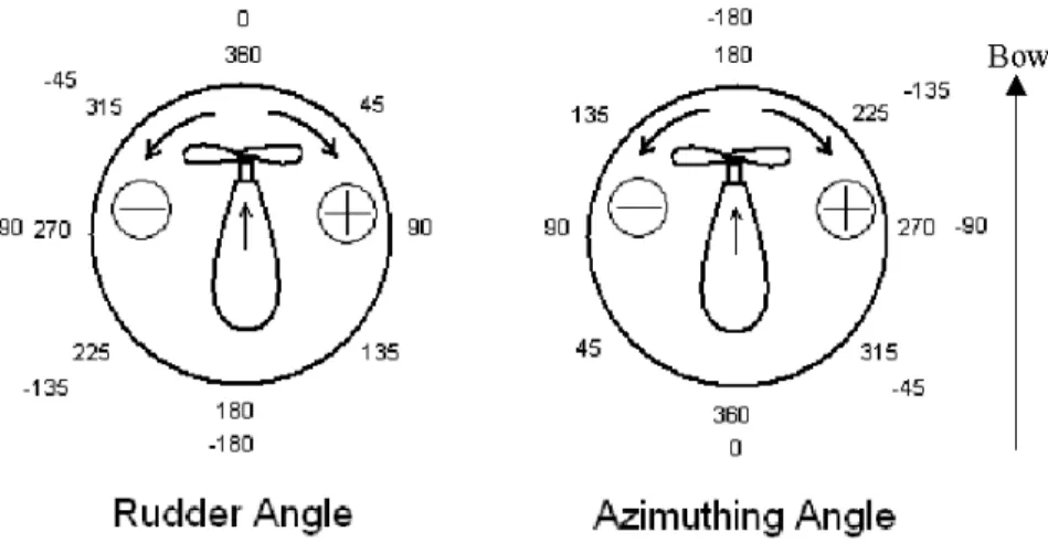
There are two terms used for describing pod angle: azimuthing angle and rudder angle. Azimuthing angle is zero when a propeller points to the stern, and rudder angle is zero when a propeller is set to make a ship going forward with respect to its heading. Both angles are positive when turning clock-wise, and negative vice versa. The following figure indicates the direction associated with azimuthing and rudder angles.
Figure 2.1: Rudder angle and azimuthing angle convention
The static testing consists of several runs of the model with different azimuthing angle, where pod A was fixed at azimuthing angle of 180 degree for every run, and pod B was set to 0, -30, -60, -90, -120, -150, -165, -170, -175, and -180 degrees for respective run. The model was also tested with increasing speed for these runs. Therefore, the relationship of Kq, KFx, and KFy as a function of J and azimuthing angle can be obtained.
The result was close to the expected final result, which would describe the three coefficients as in terms of J and azimuthing angle; however the testing only has angles between 0 to -180 degree, where the angle of pod B only pointed outward from the hull.
The character of the pod when pointing inward must also be identified, so a reference testing that has all the angles tested was required. The dynamic testing has pod B fixed at 180 degree but pod A rotated continuously over 360 degree while the model was running straight-ahead at a constant speed. This gave a relationship of the three coefficients as a function of azimuthing angle for all the angles available in pod A.
One assumption was that pod A and pod B were symmetrical so they would perform the same when they were at the symmetrical angle. For example, pod A at –30 degree would be the same as pod B at 30 degree. Based on this
assumption, static test data from pod B could be extended from –180 to 0 degree to –180 to 180 degree.
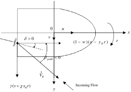
In this runs the model was towed and allowed to run straightforward only. This means that water-hull interaction was constant as the incoming flow of water or direction of ship velocity was always parallel to the model heading. On the other hand, the simulation might involve turning motion in which the heading of the ship is not necessarily parallel to the ship’s velocity, so pod modeling was introduced to explain the behavior of the ship turning in various degrees based on the straightforward runs experimented in static and dynamic testing.
The pod model used was developed by Lau and Ni (2010a). The main
development was to introduce drift angle which is the angle between direction of ship velocity and ship heading, so that the three coefficients Kq, KFx, and KFy
can be represented in terms of J , azimuthing angle, and drift angle. Usually, the simulation would prefer to use rudder angle, which is represented by “ ”, instead of azimuthing angle” ”, and drift angle is represented by “ ”.
Figure 2.2: Unparallel flow with Drift Angle
In addition, when a ship turns, resistance between hull and water changes, and therefore, thrust generated by pods might not be as efficient as in a straight motion. Thus, some factors such as wake fraction, rectification coefficient, and
0 0 podG R Vr (v x rR ) (1 w) (u y rR ) x y 0 Incoming Flow v u r
thrust deduction were taken into account where wake fraction is the reduction of the longitudinal speed along x direction, rectification coefficient is the reduction of the transverse speed in y direction, and thrust deduction lowered the thrust
produced by pods (Lau and Ni, 2010a). These factors had been built into the OSIS code and the Polaris database generator.
3 PROCEDURE FOR SIMULATION
A standard method to process podded propulsion data to be ready for the simulation in OSIS and Polaris software was developed. The overall process is illustrated in the following Figure 3.1.
Figure 3.1: Overall process for Mackinaw pod propulsion simulation The following sections describe the procedure by using examples from Mackinaw.
Acquire data from model test as .DAC files
Choose proper runs that are reasonable to describe pod performance (Kq, K , Fx KFy) as a function of
advance coefficient J and azimuthing angle
Convert .DAC files to .CSV file
Prepare the data into a proper format
Apply the prepared data to OSIS
Apply the prepared data to create Polaris data base
Verification of results (Compare OSIS/Polaris)
3.1 Acquiring Data from Model Test and Choosing Runs for the Simulation
In the model test consisted of many testing runs, the data for the testing run was recorded as .DAC files. Table 3.1 summarizes the static and dynamic run used in this analysis. The data was saved in the network share drive at IOT that can be accessed from “Iotpc\knarr\project\PJ2200”. If the testing condition was known, the proper runs can be determined directly. However, if the test run condition is not known, conversion to .CSV file might be necessary before knowing the
condition for each run. For the chosen run, the pods should be tested on different azimuthing angles and different advance speed, so that the relationship of the three coefficients Kq, KFx, and KFycan be defined in terms of advance
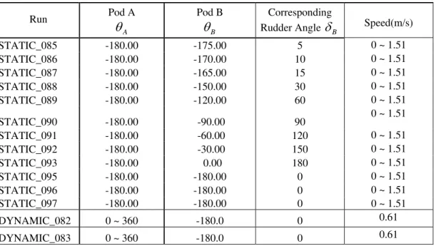
coefficient J and rudder angle . To reduce uncontrollable factors in Mackinaw model test, the chosen runs were on the testing condition where one pod was fixed and the other pod was set to different angles. For Mackinaw simulation, the run 84 to run 97 was chosen. Also reference data from dynamic test was chosen from run 82 and 83, where both run were tested in the same condition.
Combining the data from both runs will improve the accuracy of data. The use of the reference data is to extend the static data from the range [180, 0] to the range [-180,180]; however, run 84 and run 94 had pod B tested on azimuthing angle of 5 degrees, which points inward to the ship body while other runs only have the pod pointing out. This could lead to confusion when extending the data based on dynamic test because the data in region [0,-180] could also be
predicted based on the other static runs. As a result, using run 84 and 94 could lead to repetition of data from two difference sources, so they were ignored.
Table 3.1: Static and dynamic run in Mackinaw simulation
Run Pod A
A
Pod B B
Corresponding
Rudder Angle B Speed(m/s)
STATIC_085 -180.00 -175.00 5 0 ~ 1.51 STATIC_086 -180.00 -170.00 10 0 ~ 1.51 STATIC_087 -180.00 -165.00 15 0 ~ 1.51 STATIC_088 -180.00 -150.00 30 0 ~ 1.51 STATIC_089 -180.00 -120.00 60 0 ~ 1.51 STATIC_090 -180.00 -90.00 90 0 ~ 1.51 STATIC_091 -180.00 -60.00 120 0 ~ 1.51 STATIC_092 -180.00 -30.00 150 0 ~ 1.51 STATIC_093 -180.00 0.00 180 0 ~ 1.51 STATIC_095 -180.00 -180.00 0 0 ~ 1.51 STATIC_096 -180.00 -180.00 0 0 ~ 1.51 STATIC_097 -180.00 -180.00 0 0 ~ 1.51 DYNAMIC_082 0 ~ 360 -180.0 0 0.61 DYNAMIC_083 0 ~ 360 -180.0 0 0.61
Generally, choosing an appropriate run depends on the kind of runs done in the model test. For example, if there are more static tests that have pod B runs in the range [0,180] degree, extension based on dynamic test data will not be
necessary.
3.2 Conversion from .DAC file
DAC files for each test run can be converted to .CSV (Excel) files through the SWEET program, the software developed by IOT written in the Python
programming language.
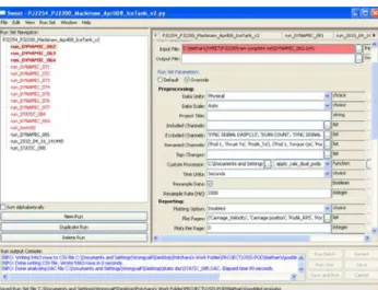
To convert static or dynamic test data of Mackinaw model test from .DAC file to .CSV, SWEET framework has to be opened. Figure 3.2 shows the template for the conversion of .DAC file to .CSV file. After SWEET is ready, click on “New Run Set File”, and browsed to
“PJ2254_PJ2200_Mackinaw_April08_IceTank_v2.py”. This is a template file made specially for converting Mackinaw data. The template shows names of the old runs in red color, which indicates that there is at least one entry that has an error. A new run can be created by duplicating one of the previous runs, and changing the new run name to be the same as the input .DAC file. The new run would also have red name indicating that some inputs are still incomplete, and there are red taps showing where the inputs are missing. Usually the error is because of an empty input or an input that has moved to a different directory. The input file’s directory has to be specified; for example,
“C:\Nathan\SWEET\PJ2200\raw complete set\DYNAMIC_083.DAC”. Also, under the Preprocessing/Custom Processor section, browse the processing code ”apply_cals_v2.py”. After this, the new run template is ready for conversion. The conversion is executed by clicking on the “Save and Run” button.
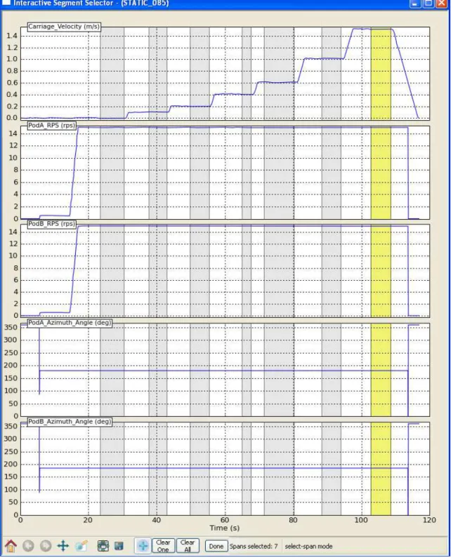
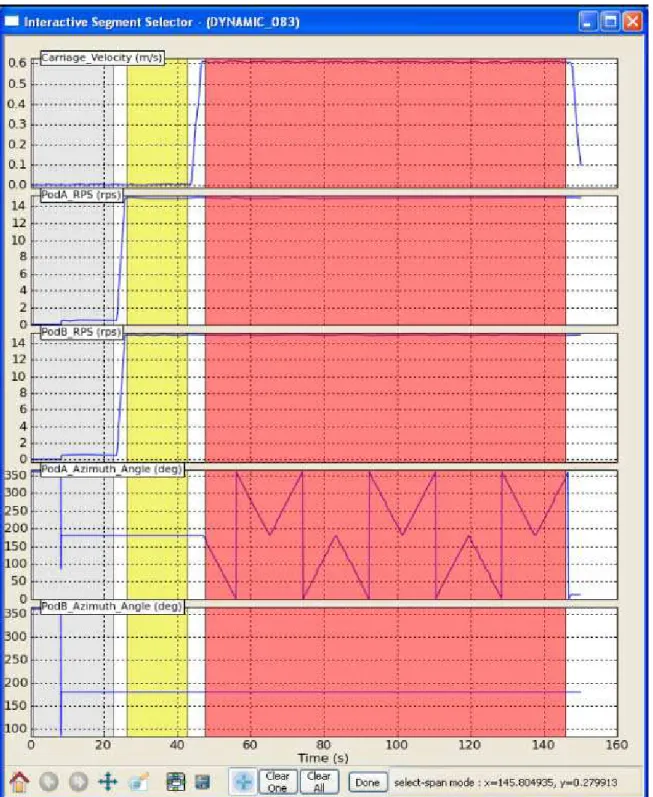
While SWEET is running, a segment selection screen is displayed (Figures 3.3 and 3.4).
Figure 3.4: Segment selector for dynamic run
SWEET will convert each selected segment to a .CSV file. So, it is necessary that appropriate segments be selected.
For static data, the model was tested with different speeds. Patterns of speed can be observed under “Carriage_Velocity” section. The important segments are
when the speed becomes steady. As in Figure 3.3, seven steady speeds were observed and selected. The output from the program is seven .CSV files saved to the same directory as “PJ2254_PJ2200_Mackinaw_April08_IceTank_v2.py”. This has to be repeated for all the run interested (e.g. runs 85, 86, 87, 88, 89, 90, 91, 92, 93, 95, 96, and 97).
The segment for dynamic runs that is important in the simulation is when the carriage speed becomes steady with azimuthing angle of one pod rotates continuously, or the red section illustrated in Figure 3.4. The .CSV file will be located in the same directory as in static runs. This has to be done for both run 82 and run 83.
More instructions about conversion of .DAC file to .CSV are given in the Analysis of Mackinaw Propulsion Test Data report.
3.3 Preparation for static and dynamic test data
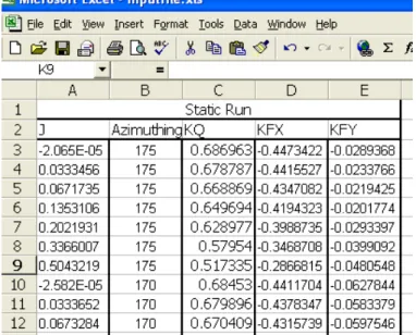
Before the data can be transferred to a simulation, they must be rearranged to a proper format. One file must contain all the information about static data, and another file must contain information about dynamic data.
There are seven .CSV files from each static run. Although each file contains detailed time-series of all data, only carriage velocity, azimuthing angle of pod B, Torque of pod B, Force in x of pod B, force in y of pod B, and RPS were
considered with the mean values of these parameters calculated for each .CSV file. Repeating this process for all seven files in all 12 static runs, there will be 7*12 sets of number. NowKq, KFx, and KFy, and advance coefficient J can be calculated where uis equal to carriage velocity, is 1002.2, and D is 0.2 m. Also, round up the numbers of azimuthing angle to integer, and line up the data in to the following format (Table 3.2):
At this point, Kq, KFx, KFy, or azimuthing angle might have opposite signs than what they suppose to be. However, they can be adjusted later after inputting the data to the Data Management program for pod simulation, a tool developed in this project.
Dynamic data can be prepared by running through the Podded Analysis program, a Matlab program that was developed prior to this project, by running
“podded_analysisV1_2openwater.m”. Before running the program, the input command of the code has to be modified for uploading the right file.
Figure 3.5 Loading file name for the Podded Analysis program As in Figure 3.5, the loading command on the sixth line loads the file “DYNAMIC_082_S3.csv” to the program. The name has to be changed
according to the file that is going to be uploaded, and the file has to be available in the same directory as “podded_analysisV1_2openwater.m”. The program
could generate the relationship of the coefficient based on multiple menus showing on Matlab command-line. In Figure 3.5, only one .CSV file is uploaded, but if there are two dynamic runs that were tested on the same condition such as run 82 and run 83, the data for both runs can be combined. To do that, the code has to be modified to:
% % %%=================================== clc
clear all
format long e;
disp('LOADING DATA SET 1'); load -ASCII DYNAMIC_082_S3.csv D_1= DYNAMIC_082_S3;
load -ASCII DYNAMIC_083_S3.csv D_2= DYNAMIC_083_S3;
D1=[D_1;D_2]; % ^ Loads data set ^
While running the program, choose pod A for analysis, and the graphs and equations of Kq, KFx, and KFy for the dynamic runs can be obtained. The
polynomial order for trend line curve fit is usually set to 6th order. This will make the trend line generated be more accurate. The output graphs show actual data points, smooth data points, and the trend line, where the actual data was
measured from the model test, smooth data was generated to remove some extreme outliers in the actual data, and the trend line and its associated equation were based on the smooth data (see Figure 3.6).
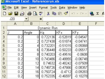
To prepare the file for pod analysis, an Excel file has to be generated manually based on the equation received as in the following format (Table 3.3).
Table 3.3: Dynamic input file format
The constant value of J has to be determined from the .CSV file, but this does not affect the simulation. Angles should be uniformly spaced from 0 to 360 by incrementing by 2 degrees. Kq, KFx, and KFy for each specific angle are
calculated by using the equation generated by the program.
3.4 OSIS simulation for Mackinaw
The prepared data can now be used as input files for OSIS. However, OSIS also has other requirements in order to start the simulation. The readers are referred to the OSIS user’s manual (Lau and Ni; 2009) for details.
One requirement for OSIS are three input files that indicates the ship properties, environmental conditions and specifics of various ship maneuvers to be
simulated. For instance, the files for Mackinaw are called “Mackinaw55InIce.ocs”, “Mackinaw55InIceFree.ocs”, and “Mackinaw55InIceNew.ocs”. These three files have to be saved under “OSIS Model Settings Files” folder.
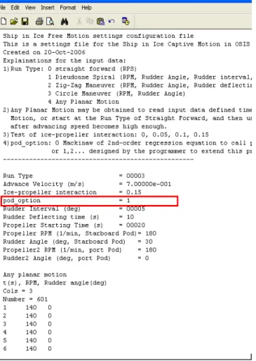
In “Mackinaw55InIceNew.ocs”, there is an option to initialize the Data
Management program within OSIS. Below a section called “Explanations for the input data”, there is a list for assigning the running type, which contains
“pod_option”. (See Figure 3.7.) When pod_option = 0, OSIS will use the default pod data from the Mackinaw, but if pod_option=1, OSIS will initiate the Data Management program, which allows the user to input pod data from a different model test.
Figure 3.7 pod_option in “Mackinaw55InIceNew.ocs”
OSIS starts by running “osis.m”. OSIS menu will then be displayed and the user can create task for “Ship Maneuvering Simulation” by selecting the model for simulation to “Mackinaw55” and setting the environment to open water in free motion mode. The type of maneuvering, pod speed, and pod angle, can be adjusted through “Free Mode button”. The simulation starts when all necessary setting is completed.
Before OSIS starts to simulate, the Data Management program will appear (Figure 3.8). The Data Management program allows the uploading of the prepared data for static test. The directory of the file should be properly addressed. Trend line order of static test data can be specified on this page, where the order is usually set to the 2nd order as it produces stable trend lines.
Figure 3.8: Input data screen
After finish entering the file name, press enter to proceed to the next screen (Figure 3.9). The performance graphs ofKq, KFx , and KFy versus azimuthing angle are displayed on this screen. Outliers and unexpected data can be
removed by clicking “Edit Data”, selecting the coefficient on the edit page (Figure 3.10), typing in the angle that has the outliers and pressing “Enter”. Run 92 of the static test, which was tested at -30 degrees, has a problem and do not gives corresponding results, so angle -30 has been dropped. J values can also be dropped if necessary. Kq, KFx , and KFy also need to be modified.
Understanding the performance graphs and physical effect of Kq , KFx , and KFy
is important for the proper editing. Usually, when a ship starts, their podded propellers have azimuthing angle at 180 degrees, as it is in tractor (or pulling) mode. There is no force in y direction acting on the pods; hence, Fy0. This leads to the first setting rule that KFy must be set to zero at 0 and 180 degrees.
In addition,KFy is positive when pod is in the range [180,360], and negative in the range [0,180]. Another rule for the setting is that KFx has to be positive at 180 degrees. Visually, it should be at its peak, as pods at 180 degrees give the best advance motion, due to maximum force achievable in x direction. OSIS would automatically cease when the ship starts to go backward. Sometimes the program will generate negative J values, but OSIS will not work in backward running in this version, so J values on the negative side will not be used in the simulation. Therefore, the existence of the negative J values in OSIS does not affect the simulation. Also, Kq is usually set to positive, but it does not affect the simulation much, as positive or negative is a matter of propeller turning direction.
Figure 3.10: Data editing screen
Dynamic data can be uploaded to data extension page (Figure 3.11). The file has to be prepared as described in Section 3.3. Order of the trend line can also be selected here, but it should be referred to the order used in the Pod Analysis program.
Figure 3.11: Data Extension screen for inputting dynamic test data
The only concern is to make sure that the reference line goes along well with the previous data. If not, the data can be adjusted through the edit page. After they are aligned along the same trend, pressing “Extend All Data” would generate the second half of the data. Nevertheless, there is one limitation in this extending function. This function accepts no more than half of the full angles. For instance, the data to be extended have to be in the range [0,180] and [180,360] only for the simulation in the azimuthing angle range [0,360].
The complete data of Kq , KFx , and KFy should look similar to those given in Figures 3.12 - 3.14, respectively.
Figure 3.12: Complete data for Kq
Figure 3.14: Complete data for KFy
3.5 Generating database for Polaris
The Polaris pod model database is a set of three look-up tables, which is used as an input file for simulation in CMS. The three databases contain coefficients Kq,
x
K , and Ky respectively. The K ’s (the coefficient of torque, force in x, and force
in y) used in OSIS and K in Polaris are calculated differently (Lau and Ni, 2010b).
To generate the three Polaris database, run the program
“form_databaseApr18.m” from Matlab, and the Data Management program shows up. The data should be modified in the same way described in OSIS, except that Kq, KFx , and KFy have to be shifted back by 180 degree to the range [-180, 180]. The program generates eight files in total. Only three files, “Kq_database.ocs”, “KFx_database.ocs”, and “KFy_database.ocs” are in the right format usable by Polaris.
3.6 Based Calculation for Data Modification with Data Management program
This section summarizes the task of the Data Management program that was used in Mackinaw simulation.
Kq, KFx , and KFy versus J, based on 10 azimuthing angles, i.e., 0, 30, 60, -90, -120, -150, -165, -170, -175, and -180 degrees, that are input. Originally there were 12 runs, but the last three run, Run 95, Run 96, and Run 97, were tested on the same azimuthing angle, so the program automatically combines them. A graphical example of the equation is given in Figure 3.15.
Figure 3.15: Example trend-line of Kqversus J for Run 97
When combining the ten trend-lines together, three 3D surfaces which represent
Kq, KFx , and KFy as a function of Jand could be obtained, where the data in
between the ten lines can be estimated based on linear interpolation (see Figure 3.16). Note that in the diagram, the angles have already been converted to positive values.
Figure 3.16: Surface representation of Kqas a function of J and
This 3D representative can be viewed in 2D for more accuracy in determining the data, as shown in Figure 3.15.
Static test data needs to be extended to cover a full range of pod angle from 0 to 360 degrees based on dynamic test data. Lau and Ni (2010a) has developed a model for data extension using Equation 3.1, where static data are the original points and dynamic data are reference points.
60 , 6 . 0 J K 60 , ref J K Extended 300 , 6 . 0 J K 300 , ref J K Figure 3.17
Equation 3.1 for data extension is expressed as: 1 1 1 2 2 1 , , , , J J J J K K K K ref ref , (3.1) Where 1 1, J
K is the original point,
2 1,
J
K is the extended point which has 2 3601, and 1
, ref J
K and KJref,2 are the reference data at the same
angles as 1 1, J K and 2 1, J K respectively.
At this point, any extreme outliers could be removed. As mentioned in Section 3.5, the angle from Run 92, which tested at angle -30 degrees, has to be removed because it gives inconsistence values.
The finished data as shown in Figure 3.18 is ready for the simulation.
Figure 3.18: Example for KFx graph with the extended data
3.7 Verification of Results
Preliminary verification of the pod model was performance by comparing the simulated turning diameter and speed during turning maneuvers between OSIS Polaris under same testing condition and ship power. The main purpose of the comparison is to determine whether the data generated from IOT and Polaris using the same pod data agree within an acceptable range.
Figure 3.19 shows the comparison of the turning diameter simulated by OSIS and Polaris, whereas a comparison of ship speed is given in Figure 3.20. Despite the difference in the hydrodynamic model representation of the ship used in OSIS and Polaris, the turning diameter and ship speed predictions agree will in both the OSIS and Polaris simulations. Details of the verification are provided in Lau and Ni (2010b).
Comparison of the Turning Diameter from Polaris' Pods (Test on Feb 19 run 1 - 180rpm) with OSIS simulation (Feb 25- matching 130.5 rpm) (Open water, one pod fixed at 0 deg, other pod set at fixed rudder angle or
both pod at fixed rudder angle)
0.0 200.0 400.0 600.0 800.0 1000.0 1200.0 1400.0 1600.0 0 10 20 30 40 50 60 70
Pod Rudder Angle (deg) Fi na l Tu rni ng Di a m et er (m )
OSIS-IOT Pod, one pod at 0 and other pod at fixde rudder angle
OSIS-IOT Pod, both pod at fixed rudder angle
Sea trial (both pod at fixed rudder angle)
Polaris Pod, one pod at 0 and other pod at fixed rudder angle
Polaris Pod, both pod at fixed rudder angle
Figure 3.19: Diameter Comparison between OSIS and Polaris
4 CONCLUSION AND RECOMMENDATION
With the procedure for podded propulsion simulation formalized, simple static and dynamic tests can be conducted and empirical model generated
automatically for numerical simulation. A tool has been developed to implement the procedure to reduce the manual processes. Nevertheless, the Data
Management program still allows for data manipulation, so the final data can still be altered.
In current version for both OSIS and Polaris database generator, wake fraction, rectification coefficient, and trust deduction, are set to some constant function or value. Different ships have different coefficients and they needed to be properly specified. Both programs still do not have any user interface to allow for new inputs of these values yet. Developing a tool to modify these parameters would greatly improve both programs capability to simulate various kinds of data.
5 REFERENCES
Lau, M. and Ni, S.Y., 2010a. Status Report: Preliminary Pod Model, NRC/IOT Report (in preparation), National Research Council of Canada, St. John’s, Newfoundland.
Lau, M. and Ni, S.Y., 2010b. IOT Pod Model Implemented in Polaris, NRC/IOT Report (in preparation), National Research Council of Canada, St. John’s, Newfoundland.
Lau, M and Ni, S.Y., 2009. “User’s Manual for OSIS (Ocean-Structure Interactions Simulator) V1.00, IOT Report LM-2009-03, Institute for Ocean Technology, National Research Council of Canada, St. John’s, Newfoundland. Akinturk, A. and Lau, M., 2010. On the Performance of Podded Propulsors, NRC/IOT Report LM-2010-05, National Research Council of Canada, St. John’s, Newfoundland.
Brazil, N., 2009. Analysis of Mackinaw Propulsion Test Data, Institute for Ocean Technology. NRC/IOT Report, SR-2009-27, National Research Council of Canada, St. John’s, Newfoundland.
NRC/IOT, 2008. Environmental Modeling – Ice, IOT Standard Test Methods 42-8595-S/GM-4, Version 3, National Research Council of Canada, St. John’s, Newfoundland.
NRC/IOT, 2004. Model Test Co-ordinate System & Unit of Measure, IOT
Standard Test Methods GM-4, Version 6, National Research Council of Canada, St. John’s, Newfoundland.