of cardiovascular death after acute coronary syndrome
The MIT Faculty has made this article openly available.
Please share
how this access benefits you. Your story matters.
Citation
Liu, Yun, Benjamin M. Scirica, Collin M. Stultz, and John V. Guttag.
“Beatquency Domain and Machine Learning Improve Prediction of
Cardiovascular Death after Acute Coronary Syndrome.” Scientific
Reports 6, no. 1 (October 6, 2016).
As Published
http://dx.doi.org/10.1038/srep34540
Publisher
Nature Publishing Group
Version
Final published version
Citable link
http://hdl.handle.net/1721.1/107813
Terms of Use
Creative Commons Attribution 4.0 International License
www.nature.com/scientificreports
Beatquency domain and machine
learning improve prediction of
cardiovascular death after acute
coronary syndrome
Yun Liu
1, Benjamin M. Scirica
2, Collin M. Stultz
1,3& John V. Guttag
3,4Frequency domain measures of heart rate variability (HRV) are associated with adverse events after a myocardial infarction. However, patterns in the traditional frequency domain (measured in Hz, or cycles per second) may capture different cardiac phenomena at different heart rates. An alternative is to consider frequency with respect to heartbeats, or beatquency. We compared the use of frequency and beatquency domains to predict patient risk after an acute coronary syndrome. We then determined whether machine learning could further improve the predictive performance. We first evaluated the use of pre-defined frequency and beatquency bands in a clinical trial dataset (N = 2302) for the HRV risk measure LF/HF (the ratio of low frequency to high frequency power). Relative to frequency, beatquency improved the ability of LF/HF to predict cardiovascular death within one year (Area Under the Curve, or AUC, of 0.730 vs. 0.704, p < 0.001). Next, we used machine learning to learn frequency and beatquency bands with optimal predictive power, which further improved the AUC for beatquency to 0.753 (p < 0.001), but not for frequency. Results in additional validation datasets (N = 2255 and N = 765) were similar. Our results suggest that beatquency and machine learning provide valuable tools in physiological studies of HRV.
Frequency domain measures of heart rate variability (HRV)1 identify patients who are at increased risk of adverse
medical outcomes2–7. Most frequency domain measures are in units of cycles per second (Hz). However,
“fre-quency” can also be measured with respect to heartbeats, in units of cycles/beat – which is sometimes expressed as “equivalent Hz” (cycles/beat * mean heart rate) in the literature8–16. In this work, our goal is to compare these
two frequency domains in the context of predicting cardiovascular death after a non-ST-elevation acute coronary syndrome (NSTEACS).
To illustrate the difference between frequency (Hz) and beatquency (cycles/beat), assume that there are two patients with constant heart rates of 60 and 120 beats per minute respectively. A frequency of 0.5 Hz corresponds to every 2 beats in the first patient but every 4 beats in the second. Use of the beatquency domain may result in more consistent predictive frequency bands between patients with different heart rates, and across different times for a given patient.
As recommended by the HRV Task Force1, most studies that analyze frequency domain HRV do so in the
frequency domain. Interestingly, however, the beatquency domain is associated with greater intra-subject and inter-subject consistency in humans8 as well as across rats and dogs15. Remarkably, to our knowledge, there have
been no published studies of the utility of beatquency in predicting adverse outcomes.
In this study we tested the hypothesis that beatquency applied to an established HRV measure, Low Frequency High Frequency (LF/HF, a ratio of energy in two bands)1 will improve prediction performance for
cardiovas-cular death post NSTEACS. We focused on frequency domain measures and LF/HF because LF/HF was the
1Institute for Medical Engineeringand Sciences, Massachusetts Institute of Technology (MIT) and Harvard-MIT
Division of Health Sciences and Technology, 77 Massachusetts Ave. Cambridge MA 02139, USA. 2TIMI Study Group,
Cardiovascular Division, Department of Medicine, Brigham and Women’s Hospital, and Harvard Medical School, 75 Francis St., Boston Ma. 02115, USA. 3Department of Electrical Engineering and Computer Science, MIT, 77
Massachusetts Ave. Cambridge MA 02139, USA. 4Computer Science and Artificial Intelligence Laboratory, MIT, 77
Massachusetts Ave. Cambridge MA 02139, USA. Correspondence and requests for materials should be addressed to C.M.S. (email: cmstultz@mit.edu)
received: 02 March 2016 Accepted: 15 September 2016 Published: 06 October 2016
best performing HRV measure on our datasets relative to other frequency domain measures (e.g., the Standard Deviation of normal RR intervals, or SDNN) in our datasets17,18. Because these original frequency bands were not
explicitly selected for optimal risk stratification, we further used machine learning to discover the frequency and beatquency bands most useful in predicting cardiovascular death post NSTEACS.
Clinical Data and Outcomes
Our work primarily utilized electrocardiographic (ECG) recordings obtained from a clinical trial of patients after NSTEACS19. The dataset consists of all 2,302 patients in the placebo arm, and contains 93 cardiovascular
deaths within the median follow-up of one year. We focused on the placebo arm because the treatment arm was prescribed ranolazine, a drug that may have anti-arrhythmic properties20 and thus affect ECG measures. We used
this dataset to compare frequency and beatquency LF/HF and to train and test machine learning models. If not otherwise indicated, all results in this work refer to this dataset. In addition, we employed two additional “holdout datasets”, for further validation of the machine learning models that were developed, using the dataset described above. These datasets are described in the Supplementary Information. Patient characteristics are reported in Table 1. For all three datasets, up to 7 days of ambulatory ECG signals recorded at 128 Hz are available for each patient. In this work, we used the first 24 hours from each patient to compute the heart rate time series. The pro-tocol was approved by the local or central Institutional Review Board at all participating centers.
Results
LF/HF in Frequency and Beatquency.
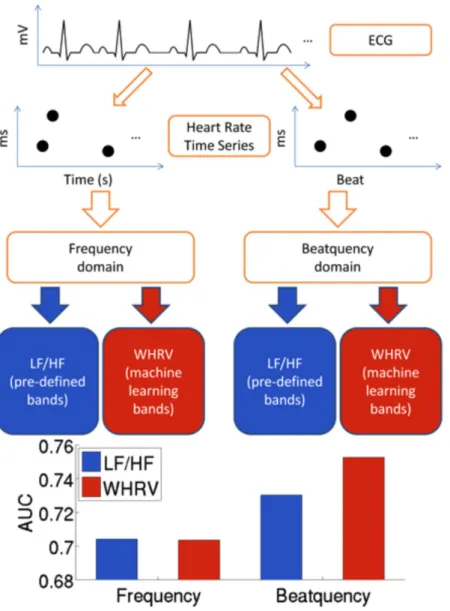
The frequency domain quantifies changes that are periodic with respect to time, while the beatquency domain quantifies changes that are periodic with respect to heartbeats. For example, a beatquency of 0.5 cycles/beat quantifies events that alternate with each heartbeat. In terms of frequency, this would correspond to 0.5 Hz at a heart rate of 60 beats per minute, but 1 Hz at a heart rate of 120 beats per minute. The calculation of frequency and beatquency domain metrics is schematically outlined in Fig. 1. The initial steps of both calculations are similar: we obtained a heart rate time series, divided it into 5-minute windows, and converted each window into each of the two frequency domains. For the “pre-defined bands” cal-culation (blue in lower half of Fig. 1), we computed the frequency LF/HF using the established LF (0.04 to 0.15 Hz) and HF (0.15 to 0.40 Hz) bands1. Diagnostic bands for beatquency LF/HF were based on a prior study that appliedLF and HF beatquency bands to normal adults as well as those with coronary artery disease and congestive heart failure: 0.03 to 0.14 (LF band) and 0.14 to 0.40 cycles/beat (HF band)14.
The Area Under the Curve (AUC) for LF/HF in frequency and beatquency in the entire cohort were sig-nificantly different, 0.713 for frequency and 0.731 for beatquency, p < 0.01 (the receiver operating charac-teristic curves are shown in Supplementary Fig. S1). Using the quartile as high-risk cutoffs for time and beat frequency (0.841 and 0.832 respectively) resulted in hazard ratios (HRs)21 of 3.7 and 4.6. After adjusting for the
Thrombolysis in Myocardial Infarction Risk Score (TRS)22, the HRs were 3.0 and 3.9 respectively. After adjusting
for TRS, ejection fraction (EF), and B-type natriuretic peptide (BNP)23, both HRs were 2.4. All HRs were
statis-tically significant (p < 0.01). The category-free net reclassification improvement24 for beatquency relative to time
frequency was 75% (95% confidence interval 42–93%).
Machine Learning (WHRV) in Frequency and Beatquency.
The LF and HF frequency and beatquency bands above were not optimized for prediction of adverse events, but were instead based on previous physio-logical studies and observations of where peaks are located in the power spectra. In this section, we evaluate a machine learning procedure to learn the predictive frequency and beatquency bands as well as the relative impor-tance (weights) of each band. We term this approach Weighted HRV (WHRV), and outline the approach in red in the lower half of Fig. 1.In the WHRV approach we first obtained a heart rate time series, divided it into 5-minute windows, and converted each window into each of the two frequency domains. Unlike the computation of frequency LF/HF where we computed the energy in pre-specified bands, here we estimated the power spectral density from 0.01 to 0.50 Hz in 0.01 increments – yielding 50 frequency bands. An identical approach applied to the heart rate time series with “beats” on the x-axis yields 50 beatquency bands ranging from 0.01 to 0.50 cycles/beat. In each case, these 50 values formed a feature vector for each patient. We first applied unsupervised approaches (Methods) to
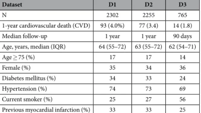
Dataset D1 D2 D3
N 2302 2255 765
1-year cardiovascular death (CVD) 93 (4.0%) 77 (3.4) 14 (1.8)
Median follow-up 1 year 1 year 90 days
Age, years, median (IQR) 64 (55–72) 63 (55–72) 62 (54–71)
Age ≥ 75 (%) 17 17 14
Female (%) 35 34 36
Diabetes mellitus (%) 34 33 24
Hypertension (%) 74 73 69
Current smoker (%) 25 27 56
Previous myocardial infarction (%) 33 33 25
www.nature.com/scientificreports/
understand if dimensionality reduction based on these frequency and beatquency features would reveal differ-ences between the two types of frequency (Table 2). Since we tested several different unsupervised methods for assessing patient risk (e.g., centered and non-centered PCA and MCE), we only report the AUCs for the method
Figure 1. Schematic of calculation of heart rate variability (HRV) metrics in frequency and beatquency.
The input ECG signal is used to compute the heart rate time series with time and beat index as the x-axis. Next, this heart rate time series is converted to the frequency or beatquency domain. The final metrics measure the energy in pre-defined bands (Low Frequency High Frequency, LF/HF), or weighted by machine learning (Weighted HRV, WHRV).
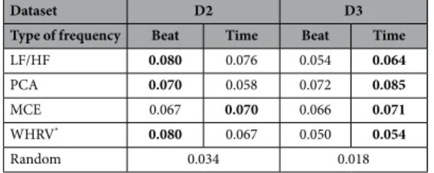
Dataset D2 D3
Type of frequency Beat Time Beat Time
LF/HF 0.725 0.710 0.733 0.709
PCA 0.726 0.620 0.680 0.669 MCE 0.687 0.652 0.767 0.713 WHRV* 0.728 0.691 0.738 0.679
Random 0.500
Table 2. Prediction performance (AUC, area under receiver operating characteristic curve) for cardiovascular death. Bold indicates the higher AUC in each pair (time vs beat). *Indicates WHRV (the
supervised approach) was trained on dataset D1 and the reported results are averaged over patients that the model was not trained on.
that yielded the best results in Table 2. (Details of the performance of each of the methods we investigated are shown in Supplementary Figs S3–S5). In all cases (particularly in the larger validation dataset D2), the discrim-inatory performance was improved in beatquency relative to frequency (see Table 2). Furthermore, these data demonstrate that these techniques can perform remarkably well, yielding AUCs as high as 0.726 in the larger validation dataset D2 (using principle component analysis), and as high as 0.767 in the smaller dataset D3 (using minimum curvilinear embedding25). The fact that dimensionality reduction using beatquency features can yield
improved performance argues that a combined approach that uses both a dimensionality reduction approach coupled with supervised learning may further improve the performance of the beatquency approach.
Based on these encouraging findings, we adopted a supervised learning approach by feeding the feature vec-tors to an L1-regularized logistic regression algorithm, which selects the most important features (frequency or beatquency bands). The algorithm outputs a weight vector, which quantifies the relative importance of each fre-quency band in the prediction. For each patient, the WHRV is the scalar valued dot product of the feature vector with the weight vector, and higher values indicate higher risk. The machine learning protocol is described in more detail in the Methods.
We trained separate models on each of 1,000 randomly chosen training sets and evaluated the results averaged across the 1,000 test sets to ensure results were not dependent on the randomness of each split (Methods). The AUC for beatquency WHRV was significantly higher than that of frequency in the test sets taken from dataset D1 (Table S2, 0.753 versus 0.704, p < 0.001). Applying the same trained models to two additional holdout sets demonstrated similar trends (0.728 versus 0.691, and 0.738 versus 0.679, p < 0.001, see Table 2). Moreover, while machine learning left the AUC of frequency LF/HF unchanged, it increased the AUC of beatquency LF/HF using test sets from dataset D1 (0.704 to 0.730, p < 0.001, Table S2) and in the validation sets (Table 2). These values are significantly higher than those of another HRV metric, SDNN (standard deviation of NN intervals).
Lastly we note that since the AUC may be deceptive in the setting of significant class imbalance (i.e., a rela-tively small number of positive examples)16,25–27, we also calculated the AUPR for each of the predictive methods
we examined (Table 3). While the AUPRs on the smaller validation dataset, D3, do not show an improvement in performance when a beat-space analysis is used, in most cases the performance on the larger dataset, D2, shows an improvement in the beatquency domain. The fact that the overall AUPRs are low highlights the fact that there is room for improvement with respect to development of a model with true clinical utility. Nevertheless, we were encouraged by the fact that beatquency improves the AUC in all of our applied methods.
To further explore the utility of our methods, we evaluated them on patients who would not be identified as high risk by TRS (TRS ≤ 4). The AUC for beatquency WHRV increased to 0.773 in this population, and this per-formance was preserved in both males (0.772) and females (0.758) (Table S2). Similarly, these AUCs were higher than that those in frequency, and substantially higher than SDNN.
We present the HRs of the models before and after adjusting for clinical variables in Table 4. The unadjusted HR’s were 3.70 and 5.19 for frequency and beatquency respectively. In multivariable analysis, the HRs were 3.13 and 4.38 after adjusting for TRS, and 1.99 and 2.91 after adjusting for TRS, EF and BNP. After adjusting for all three variables, the WHRV beatquency metric had a confidence interval that excluded 1. In addition, the adjusted HR using machine learning was higher than those using pre-defined bands for beatquency; i.e., the LF/HF beatquency HR is 2.45 vs. a beatquency WHRV HR of 2.91 (where only the latter has a 95% CI that excludes 1). This was not the case when machine learning was applied to the frequency domain; i.e., the LF/HF frequency HR is 2.28 vs. a WHRV frequency HR of 1.99.
Dataset D2 D3
Type of frequency Beat Time Beat Time
LF/HF 0.080 0.076 0.054 0.064
PCA 0.070 0.058 0.072 0.085
MCE 0.067 0.070 0.066 0.071
WHRV* 0.080 0.067 0.050 0.054
Random 0.034 0.018
Table 3. Prediction performance (AUPR, area under precision recall curve) for cardiovascular death. Bold
indicates the higher AUC in each pair (time vs beat). *Indicates WHRV (the supervised approach) was trained
on dataset D1 and the reported results are averaged over patients that the model was not trained on.
WHRV HR (95% CI) LF/HF HR (95% CI)
Beat Time Beat Time
Unadjusted 5.19 (2.60,9.45) 3.70 (1.98,6.76) 4.44 (2.51,7.92) 3.73 (2.20,6.68) Adj. for TRS 4.38 (2.23,8.62) 3.13 (1.72,5.89) 3.74 (2.01,7.07) 3.09 (1.73,5.84) Adj. for TRS,EF,BNP† 2.91 (1.05,8.68) 1.99 (0.69,5.73) 2.45 (0.98,6.90) 2.28 (0.86,6.72)
Table 4. Hazard Ratio (HR) averaged over 1,000 test sets in D1. 95% confidence intervals (CI) reported in
parenthesis. Bold indicates the highest HR in each row (p < 0.001 for unadjusted and adjusted for TRS; in the last row only WHRV in beatquency has a CI that does not include 1). †In 7 out of 1,000 test sets, less than 30%
www.nature.com/scientificreports/
The results above used the quartile as the high-risk cutoff. To explore the utility of using other cutoffs, we com-pared the positive predictive values and negative predictive values of these four metrics over all possible cutoffs from the 5th to the 95th percentile, in increments of 10 percentiles (Supplementary information, Figs S7 and S8).
Beatquency WHRV demonstrated the highest positive predictive value from the 25th to the 85th percentile,
demonstrating robustness to the choice of the cutoff. The negative predictive values of all the measures were above 96% at all cutoffs, suggesting utility in identifying patients who are not at high-risk.
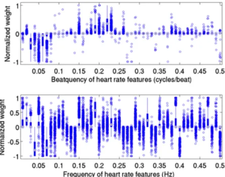
Each of the 1,000 randomly chosen training sets generated a distinct weight vector. We observed a greater consistency in beatquency features compared to frequency in these 1,000 weight vectors: the average stand-ard deviation of the normalized beatquency feature weights is less than half that of the frequency value (Fig. 2, 0.057 versus 0.153, p < 0.001). Moreover, beatquencies between 0.03–0.07 cycles/beat have consistently negative weights across the 1,000 different models – suggesting that high power in these bands is associated with decreased rate of one-year cardiovascular death. By contrast, beatquencies between 0.18–0.24 cycles/beat are associated with positive weights – suggesting that high power in these bands is associated with an increased rate of one-year cardiovascular death. Since the models built using frequency features show much more variation across the 1,000 different models, it is difficult to make reliable inferences about the relative importance of different frequency bands.
Discussion
Since the autonomic nervous system is an important regulator of heart rate, analysis of heart rate variability can provide useful information about autonomic tone. Quantitative metrics like HRV that provide insight into the autonomic tone are often calculated using the frequency domain. Frequency domain HRV metrics have been shown to provide useful prognostic information after a myocardial infarction in multiple studies2–7 and after
NSTEACS17,18. However, though frequency HRV measures are associated with elevated risk after NSTEACS,
these risk measures miss significant numbers of deaths18. Our results suggest that quantifying LF/HF in terms of
beatquency instead of frequency improves the ability to identify high-risk patients after a NSTEACS.
Analysis of the relationship between the frequency spectrum and the average heart rate provides insight into the improved performance of measures that are calculated from the beatquency spectrum. In a study by Perini
et al., young male subjects exercised on a cycle ergometer at pre-specified exercise intensities28. With increasing
exercise intensity, the center frequency of the HF band increased from 0.24 to 0.48 Hz (Fig. 3). By contrast, our estimate of the center frequency of the corresponding HF band in beatquency varies from 0.17 to 0.19 cycles/beat over the same range of heart rates (Fig. 3). Because beatquency bands are less sensitive to changes in average heart rate, they allow patients and ECG segments with different average heart rates to be directly compared.
Because the location of the HF band is influenced by the respiratory rate29,30, and heart rate and respiratory
rate are correlated, beatquency may be correcting for respiratory rate. There exist sophisticated algorithms to extract the respiratory rate from the ECG, for example in ref. 31, and to adjust the frequency bands based on the respiratory rate32,33. These methods may improve risk stratification further, however we note that the simplicity
of beatquency enables it to be easily applied to existing large HRV datasets and also to new HRV studies without additional equipment or expert oversight in selecting appropriate frequency bands.
Figure 2. Boxplot of normalized weights of frequency and beatquency machine learning models trained on the same 1,000 training splits. Quartiles are represented by the edges of lines, box, and central dot, while circles
The fact that beatquency WHRV (using machine learning) outperformed beatquency LF/HF (using pre-defined bands) highlights the benefit of adopting a data-driven, machine learning approach to analyzing heart rate spectra. An analysis of the weights of the beatquency bands finds trends that are similar to what has been observed with trends in standard frequency LF/HF measurements. In particular, the signs of the beatquency bands weights (negative at 0.03 to 0.07 cycles/beat and positive at 0.18 to 0.24 cycles/beat) are consistent with the notion that in patients post myocardial infarction, lower values of LF/HF are associated with adverse events in some patient populations34. Our data also demonstrate that using features derived from the beatquency spectrum yields
logistic regression models that have improved performance relative to models derived from the frequency spec-trum. Thus beatquency may also have utility in other machine learning models that leverage frequency domain ECG features, such as for arrhythmia classification35. One limitation of our observations is that we used Holter
data that were collected at the standard frequency of 128 Hz. Higher sampling rates may improve the accuracy of our measured RR intervals and further improve results, especially for standard frequency domain HRV measures.
Applying machine learning to frequency bands does not yield a significant improvement in either the AUC or the unadjusted or adjusted hazard ratios relative to the pre-defined frequency bands. That machine learning improves risk stratification with beatquency bands but not frequency bands can be explained by the greater con-sistency of feature weights in beat- compared to frequency. Since differences in average heart rate are associated with shifts in the frequency domain spectra, the predictive frequencies may differ between patients and across time for each patient. Thus frequency features may not generalize across patients or even between segments of dif-ferent heart rates for the same patient. This leads to unchanged or even decreased performance despite an attempt to learn the predictive frequencies.
Overall, applying beatquency and machine learning to heart rate variability metrics improves our ability to identify patients at elevated risk of cardiovascular death post NSTEACS. Our machine learning approach in beatquency also reveals predictive bands that can be studied in more detail in physiological studies, and more generally, showcases a data driven approach to selecting frequency bands for analysis. Our discrimina-tory results could be improved further by including other variables (both based on HRV and otherwise) in the machine-learning model. As already mentioned, the objective of this work was to compare the ability of two different methods for representing the heart rate time series. Our data demonstrate the relative power of a beatquency approach for identifying patients at high risk of death post ACS. Effective risk metrics may arise from models that combine beatquency variables with other non-linear metrics that have been applied medical data36–38.
Beyond predicting patient risk, future work would be required to further validate these risk metrics and to find the most effective therapies in high risk patients highlighted by these risk metrics.
Methods
Frequency LF/HF.
We first segmented the 24-hour long ECG signal to find individual heartbeats, and used the Signal Quality Index39 to extract the normal beats. To ensure that only normal beats were analyzed, the two beatsadjacent to each abnormal beat were removed as well. We performed manual checks to ensure these segmentation and beat classification steps were appropriate. These steps are described in detail in our previously published work40.
To calculate the frequency LF/HF we divided the heart rate time series into 5-minute intervals and estimated the power spectral density in the frequency domain. There are many ways to compute the frequency domain power spectrum; we use the Lomb-Scargle periodogram, which provides a natural way to handle unevenly sam-pled data41,42. For the RR time series, this uneven sampling has two sources: the inherent heart rate variations in
the underlying ECG, and the removal of ectopic beats or artifacts. We then computed the ratio of the energy in the LF band to the HF band for each 5-minute window, and defined the median value of all these LF/HF ratios to be the LF/HF for that patient. A low LF/HF ratio is known to be associated with poorer prognosis34.
Figure 3. Location of high frequency band in exercising subjects. Frequency data are from ref. 28;
beatquencies are estimated by dividing the frequency value by the heart rate in Hz. Error bars represent standard error.
www.nature.com/scientificreports/
Beatquency LF/HF.
Frequency LF/HF was obtained from the power spectrum of the heart rate timeseries, where the time points of the beats were used as a temporal reference in the Lomb-Scargle periodogram.
Beatquency LF/HF was also obtained from the power spectrum of the heart rate time series, however, the
heart-beat indices were used as the “temporal” reference. Where heart-beats or parts of the signal were removed (as described in the previous section), the number of removed beats was estimated using the average time intervals of the heart-beats immediately adjacent to the gap18. As mentioned in the results section, diagnostic bands for beatquency
LF/HF were based on a prior study that applied LF and HF beatquency bands to normal adults as well as those with coronary artery disease and congestive heart failure: 0.03 to 0.14 (LF band) and 0.14 to 0.40 cycles/beat (HF band)14. The remaining steps in beatquency LF/HF computation were identical to the frequency construction.
Figure 1 compares the two approaches.
We verified that frequency and beatquency bands were meaningfully different by computing the correlation coefficient of the LF and HF bands in frequency with bands in beatquency. The most similar beatquency bands had correlations of 0.63 (0.04 to 0.13) and 0.81 (0.10 to 0.37) for frequency LF and HF respectively. These corre-spond to 40% and 66% of the explained variance, respectively.
Machine Learning.
In this section, we describe a machine learning procedure to learn predictive frequency and beatquency bands as well as the relative importance (weights) associated with each band. First, we will describe the feature construction for each patient, where each feature is related to a frequency or beatquency band. These features were then used to train a model, which outputs a weight vector and a prediction for each patient. The weight vector quantifies the importance of each frequency band in the prediction, and for each patient the prediction was the dot product of the feature vector with the weight vector. We term the resulting scalar-valued prediction the Weighted HRV (WHRV).The initial steps were similar to the LF/HF computation (Fig. 1). We obtained a heart rate time series, divided it into 5-minute windows, and converted each window into the frequency domain. Unlike the computation of frequency LF/HF where we computed the energy in pre-specified bands, here we estimated the power spectral density from 0.01 to 0.50 Hz in 0.01 increments. After this was done for all 5-minute windows for that patient, we defined each feature as the 90th percentile of the power for that frequency over all 5-minute windows. This
90th percentile value was used in previous ECG measures, and is intended to capture the maximum variability in
a particular frequency while excluding outliers17,18. These 50 features quantify the heart rate variability at each
frequency from 0.01 to 0.50 Hz.
The beatquency features were constructed in a similar fashion, except that beat indices were used as the tem-poral reference in the Lomb-Scargle periodogram instead of time points. The other steps of preprocessing (i.e., division into 5-minute windows, and taking the 90th percentile) were identical. The 50 features obtained quantify
the heart rate variability in 50 beatquency bands from 0.01 to 0.50 cycles/beat. We visualized these frequency and beatquency features using principle component analysis (PCA) and non-centered Minimum Curvilinear Embedding (MCE, a type of topological-based nonlinear kernel PCA25, and found promising discriminatory
performance (Tables 2 and 3, Supplementary Figs S3–S5). These unsupervised results encouraged us to apply supervised machine learning methods, as described in the next sections.
The machine learning protocol consists of randomly dividing the initial dataset into a training set and a test set in a 2:1 ratio, stratified by outcome; i.e., training sets and test sets have the same percentage of cardiovascu-lar deaths. A L1-regularized logistic regression model (Equation 1) as implemented in LIBLINEAR43, was then
trained on the training set and tested on the test set.
∑
∑
= + + + + − ∈ − + ∈ − − +ˆw argmin w C log(1 e ) C log(1 e )
(1) w w x w x i D y j D y 1 i T i j T j
where ˆw is the optimum weight vector that minimizes the expression in square braces in equation 1, ||• ||1 is the L1
norm, D− and D+ are data (patients) in the negative (alive) and positive (dead) classes, C− and C+ are cost
param-eters for the two classes, yi and yj are the scalar class labels for patients i and j, and assumes a value of either − 1 or + 1.
The variables xi and xj denote the feature vectors for patients i and j, respectively.
Because we expected only a relatively small subset of the frequency domain to contain pertinent prognos-tic information, we applied L1 regularization to perform implicit feature selection. Within the training set, five
repeats of 5-fold cross validation were used to optimize the cost parameters C− and C+, for patients in the
neg-ative (alive) and positive (dead) classes respectively. This asymmetric cost was necessary because only 4% of the patients experienced an event. C− is optimized from the range 10−6 to 10−2 in exponential steps, while keeping
C+ = k * C−, where k is the class imbalance ratio. We standardized each frequency domain feature by subtracting
the mean value of that feature and dividing by its standard deviation across all patients.
Evaluation of Machine Learning Models.
We evaluated the performance of WHRV by randomly split-ting the dataset into a training set and a test set in a 2:1 ratio. This training/test split procedure ensures that mod-els are evaluated based on their performance on patients that the modmod-els have previously not “seen”. We trained a machine learning model on the training set and measured the discriminatory performance on the test set using the area under the receiver operating characteristic curve (AUC)44 for the outcome of cardiovascular death within1 year. The AUC can be interpreted as a probability: given a patient who eventually experienced the outcome of interest (e.g. cardiovascular death within 1 year) and another who did not, what is the probability that the model ranks the patient who died as at a higher risk than the patient who did not45?
We repeated this training/test split 1,000 times to reduce the effects of selecting an overly optimistic or pes-simistic test set, i.e. we constructed 1,000 training sets and 1,000 test sets. We report results averaged over the
1,000 test sets. To evaluate the performance of these models in the additional holdout datasets (as described in the supplement), we computed the AUC for each of the 1,000 models in the holdout dataset, and report the average AUC. In addition, we also evaluated the trained models on two additional datasets (reported in the Supplement) and summarize the results in the main text.
The relative importance of the 50 frequency and beatquency features were analyzed across the 1,000 different models by dividing the weight of each feature by the maximum absolute weight in each model (i.e., the largest absolute value of the normalized weights will be 1). We estimated the variation in feature weights by first comput-ing the standard deviation of each normalized feature weight across all 1,000 models to obtain a standard devia-tion for each feature. We summarized these 50 standard deviadevia-tions by taking the average. A higher value indicates a higher variation of feature weights across different training sets.
Comparison with Clinical Measures.
We evaluated the performance of our model relative to several clini-cal variables, the Thrombolysis In Myocardial Infarction Risk Score22 (TRS), left ventricular ejection fraction (EF),and B-type natriuretic peptide23 (BNP). The TRS summarizes the effects of numerous risk factors, including age,
elevated biomarkers, and presence of coronary artery disease. The score is defined as the number of risk factors (out of 7) that a person has, and thus ranges from 0 to 7. Patients with TRS ≥ 5 are considered to be at high risk22.
EF quantifies the fraction of blood ejected in each cardiac cycle; we use ≤ 40% as the threshold for high risk18.
BNP is a blood marker indicating ventricular stretch, and > 80 pg/ml is considered a high-risk cutoff 23. Because
EF and BNP were only measured in 47% of the patients18, we build separate multivariable models: a model that
includes only TRS and uses all the patients, and a model that includes TRS, EF, and BNP, and uses only the patients with measured values of both EF and BNP.
Statistical Analysis.
In the LF/HF section, we assess the statistical significance of differences between the AUCs of two metrics (frequency and beatquency versions) on the entire dataset46. In addition, we computed the category-freenet reclassification improvement to assess the difference between the frequency and beatquency LF/HF24.
In the machine learning section, we assess the difference of AUCs across 1,000 test sets using a two-tailed paired t-test. Because of the known issues with the AUC in imbalanced datasets16,25–27, we also report the area under the
pre-cision recall curve (AUPR). Because dataset D3 has few outcomes (distinct from low proportion of outcomes), flipping the prediction in a single positive patient can cause a large change in precision and recall and “raggedness” in the pre-cision recall curve. Thus, we place more emphasis on performance measurements on the larger datasets D1 and D2.
In addition, we computed the hazard ratio (HR) of the different HRV risk metrics using the Cox proportional hazards regression model21. We dichotomized the continuous machine learning predictions at the upper quartile of
each test set; thus the HR indicates the hazard ratio of the upper quartile compared to the remaining patients. We adjusted the HR for TRS, EF, and BNP using binary variables defined by the high-risk cutoffs described in the pre-vious section. Thus, we present three HRs: unadjusted, adjusted for TRS, and adjusted for all of TRS, EF, and BNP.
References
1. Heart rate variability. Standards of measurement, physiological interpretation, and clinical use. Task Force of the European Society of Cardiology and the North American Society of Pacing and Electrophysiology. Eur Heart J 17, 354–381 (1996).
2. Bigger, J. T. et al. Frequency domain measures of heart period variability and mortality after myocardial infarction. Circulation 85, 164–171 (1992).
3. Bigger, J. T., Fleiss, J. L., Rolnitzky, L. M. & Steinman, R. C. Frequency domain measures of heart period variability to assess risk late after myocardial infarction. Journal of the American College of Cardiology 21, 729–736 (1993).
4. Lanza, G. A. et al. Prognostic role of heart rate variability in patients with a recent acute myocardial infarction. The American journal
of cardiology 82, 1323–1328 (1998).
5. Huikuri, H. V. et al. Fractal correlation properties of RR interval dynamics and mortality in patients with depressed left ventricular function after an acute myocardial infarction. Circulation 101, 47–53 (2000).
6. Tapanainen, J. M. et al. Fractal analysis of heart rate variability and mortality after an acute myocardial infarction. The American
journal of cardiology 90, 347–352 (2002).
7. Stein, P. K., Domitrovich, P. P., Huikuri, H. V. & Kleiger, R. E. Traditional and nonlinear heart rate variability are each independently associated with mortality after myocardial infarction. Journal of cardiovascular electrophysiology 16, 13–20 (2005).
8. Lisenby, M. J. & Richardson, P. C. The Beatquency Domain: an unusual application of the fast Fourier transform. IEEE Trans Biomed
Eng 24, 405–408, doi: 10.1109/tbme.1977.326155 (1977).
9. Pagani, M. et al. Power spectral density of heart rate variability as an index of sympatho-vagal interaction in normal and hypertensive subjects. Journal of hypertension. Supplement: official journal of the International Society of Hypertension 2, S383–S385 (1984).
10. Pagani, M. et al. Simultaneous analysis of beat by beat systemic arterial pressure and heart rate variabilities in ambulatory patients.
Journal of hypertension. Supplement: official journal of the International Society of Hypertension 3, S83–S85 (1985).
11. Nakata, A. et al. Spectral analysis of heart rate, arterial pressure, and muscle sympathetic nerve activity in normal humans. American
Journal of Physiology-Heart and Circulatory Physiology 274, H1211–H1217 (1998).
12. Sei, H., Enai, T., Chang, H.-Y. & Morita, Y. Heart rate variability during sleep in Down’s syndrome. Physiology & behavior 58, 1273–1276 (1995).
13. Takei, Y. Relationship between power spectral densities of PP and RR intervals. The Annals of physiological anthropology 11, 325 (1992).
14. Wu, G., Shen, L., Tang, D., Zheng, D. & Poon, C.-S. In Engineering in Medicine and Biology Society, 2006. EMBS'06. 28th Annual
International Conference of the IEEE. 3557-3560 (IEEE).
15. Rubini, R., Porta, A., Baselli, G., Cerutti, S. & Paro, M. Power spectrum analysis of cardiovascular variability monitored by telemetry in conscious unrestrained rats. J Auton Nerv Syst 45, 181–190 (1993).
16. Davis, J. & Goadrich, M. In Proceedings of the 23rd international conference on Machine learning. 233–240 (ACM).
17. Syed, Z. et al. Relation of death within 90 days of non-ST-elevation acute coronary syndromes to variability in electrocardiographic morphology. Am J Cardiol 103, 307–311, doi: 10.1016/j.amjcard.2008.09.099 (2009).
18. Liu, Y. et al. ECG Morphological Variability in Beat Space for Risk Stratification After Acute Coronary Syndrome. Journal of the
www.nature.com/scientificreports/
19. Morrow, D. A. et al. Effects of ranolazine on recurrent cardiovascular events in patients with non–st-elevation acute coronary syndromes. JAMA: the journal of the American Medical Association 297, 1775–1783 (2007).
20. Scirica, B. M. et al. Effect of Ranolazine, an Antianginal Agent With Novel Electrophysiological Properties, on the Incidence of Arrhythmias in Patients With Non–ST-Segment–Elevation Acute Coronary Syndrome Results From the Metabolic Efficiency With Ranolazine for Less Ischemia in Non–ST-Elevation Acute Coronary Syndrome–Thrombolysis in Myocardial Infarction 36 (MERLIN-TIMI 36) Randomized Controlled Trial. Circulation 116, 1647–1652 (2007).
21. Cox, D. R. Regression models and life-tables. Journal of the Royal Statistical Society. Series B (Methodological) 34, 187–220 (1972).
22. Antman, E. M. et al. The TIMI risk score for unstable angina/non-ST elevation MI: A method for prognostication and therapeutic decision making. Jama 284, 835–842 (2000).
23. de Lemos, J. A. et al. The prognostic value of B-type natriuretic peptide in patients with acute coronary syndromes. N Engl J Med
345, 1014–1021, doi: 10.1056/NEJMoa011053 (2001).
24. Pencina, M. J., D’Agostino, R. B. & Steyerberg, E. W. Extensions of net reclassification improvement calculations to measure usefulness of new biomarkers. Statistics in medicine 30, 11–21 (2011).
25. Cannistraci, C. V., Alanis-Lobato, G. & Ravasi, T. Minimum curvilinearity to enhance topological prediction of protein interactions by network embedding. Bioinformatics 29, i199–i209 (2013).
26. Yang, Y., Lichtenwalter, R. N. & Chawla, N. V. Evaluating link prediction methods. Knowl. Inf. Syst. 45, 751–782, doi: 10.1007/ s10115-014-0789-0 (2015).
27. Daminelli, S., Thomas, J. M., Durán, C. & Cannistraci, C. V. Common neighbours and the local-community-paradigm for topological link prediction in bipartite networks. New Journal of Physics 17, 113037 (2015).
28. Perini, R., Orizio, C., Baselli, G., Cerutti, S. & Veicsteinas, A. The influence of exercise intensity on the power spectrum of heart rate variability. European journal of applied physiology and occupational physiology 61, 143–148 (1990).
29. Brown, T. E., Beightol, L. A., Koh, J. & Eckberg, D. L. Important influence of respiration on human R-R interval power spectra is largely ignored. J Appl Physiol (1985) 75, 2310–2317 (1993).
30. Pitzalis, M. V. et al. Effect of respiratory rate on the relationships between RR interval and systolic blood pressure fluctuations: a frequency-dependent phenomenon. Cardiovasc Res 38, 332–339 (1998).
31. Bailon, R., Sornmo, L. & Laguna, P. A robust method for ECG-based estimation of the respiratory frequency during stress testing.
IEEE transactions on bio-medical engineering 53, 1273–1285 (2006).
32. Bailón, R., Laguna, P., Mainardi, L. & Sornmo, L. In Engineering in Medicine and Biology Society, 2007. EMBS 2007. 29th Annual
International Conference of the IEEE. 6674–6677 (IEEE).
33. Goren, Y., Davrath, L. R., Pinhas, I., Toledo, E. & Akselrod, S. Individual time-dependent spectral boundaries for improved accuracy in time-frequency analysis of heart rate variability. IEEE transactions on bio-medical engineering 53, 35–42 (2006).
34. Singh, N., Mironov, D., Armstrong, P. W., Ross, A. M. & Langer, A. Heart rate variability assessment early after acute myocardial infarction. Pathophysiological and prognostic correlates. GUSTO ECG Substudy Investigators. Global Utilization of Streptokinase and TPA for Occluded Arteries. Circulation 93, 1388–1395 (1996).
35. Asl, B. M., Setarehdan, S. K. & Mohebbi, M. Support vector machine-based arrhythmia classification using reduced features of heart rate variability signal. Artificial intelligence in medicine 44, 51–64 (2008).
36. Kovatchev, B. P. et al. Sample asymmetry analysis of heart rate characteristics with application to neonatal sepsis and systemic inflammatory response syndrome. Pediatric research 54, 892–898 (2003).
37. Sleigh, J. & Donovan, J. Comparison of bispectral index, 95% spectral edge frequency and approximate entropy of the EEG, with changes in heart rate variability during induction of general anaesthesia. British journal of anaesthesia 82, 666–671 (1999).
38. Pincus, S. M., Gladstone, I. M. & Ehrenkranz, R. A. A regularity statistic for medical data analysis. Journal of Clinical Monitoring 7, 335–345, doi: 10.1007/bf01619355 (1991).
39. Li, Q., Mark, R. G. & Clifford, G. D. Robust heart rate estimation from multiple asynchronous noisy sources using signal quality indices and a Kalman filter. Physiological measurement 29, 15 (2008).
40. Syed, Z. et al. Spectral energy of ECG morphologic differences to predict death. Cardiovasc Eng 9, 18–26, doi: 10.1007/s10558-009-9066-3 (2009).
41. Lomb, N. R. Least-squares frequency analysis of unequally spaced data. Astrophysics and space science 39, 447–462 (1976). 42. Clifford, G. D. & Tarassenko, L. Quantifying errors in spectral estimates of HRV due to beat replacement and resampling. Biomedical
Engineering, IEEE Transactions on 52, 630–638 (2005).
43. Fan, R.-E., Chang, K.-W., Hsieh, C.-J., Wang, X.-R. & Lin, C.-J. LIBLINEAR: A library for large linear classification. The Journal of
Machine Learning Research 9, 1871–1874 (2008).
44. Bradley, A. P. The use of the area under the ROC curve in the evaluation of machine learning algorithms. Pattern recognition 30, 1145–1159 (1997).
45. Hanley, J. A. & McNeil, B. J. The meaning and use of the area under a receiver operating characteristic (ROC) curve. Radiology 143, 29–36 (1982).
46. DeLong, E. R., DeLong, D. M. & Clarke-Pearson, D. L. Comparing the areas under two or more correlated receiver operating characteristic curves: a nonparametric approach. Biometrics, 837–845 (1988).
Acknowledgements
This work was supported by the Agency of Science, Technology, and Research (A*STAR), Singapore, Quanta Computer, Taiwan, and General Electric, USA. The clinical trial was supported by CV Therapeutics (now Gilead Sciences).
Author Contributions
Y.L., C.M.S. and J.V.G. conceived the study and wrote the manuscript. B.M.S. provided feedback and reviewed the manuscript.
Additional Information
Supplementary information accompanies this paper at http://www.nature.com/srep Competing financial interests: The authors declare no competing financial interests.
How to cite this article: Liu, Y. et al. Beatquency domain and machine learning improve prediction of
This work is licensed under a Creative Commons Attribution 4.0 International License. The images or other third party material in this article are included in the article’s Creative Commons license, unless indicated otherwise in the credit line; if the material is not included under the Creative Commons license, users will need to obtain permission from the license holder to reproduce the material. To view a copy of this license, visit http://creativecommons.org/licenses/by/4.0/