Inventory credit to enhance food security in Africa

HAL Id: hal-02018715

https://hal.archives-ouvertes.fr/hal-02018715v2

Preprint submitted on 16 Nov 2020

HAL is a multi-disciplinary open access archive for the deposit and dissemination of sci-entific research documents, whether they are pub-lished or not. The documents may come from teaching and research institutions in France or abroad, or from public or private research centers.

L’archive ouverte pluridisciplinaire HAL, est destinée au dépôt et à la diffusion de documents scientifiques de niveau recherche, publiés ou non, émanant des établissements d’enseignement et de recherche français ou étrangers, des laboratoires publics ou privés.

Inventory credit to enhance food security in Africa

Tristan Le Cotty, Elodie Maitre d’Hotel, Subervie Julie

To cite this version:

Tristan Le Cotty, Elodie Maitre d’Hotel, Subervie Julie. Inventory credit to enhance food security in Africa. 2019. �hal-02018715v2�

I

nvent

or

y

Cr

edi

t

t

o

Enhanc

e

Food

Sec

ur

i

t

y

i

n

Af

r

i

c

a

T

r

i

s

t

an

L

e

C

ot

t

y

El

odi

e

Mai

t

r

e

d’

Hot

e

l

&

J

ul

i

e

Sube

r

v

i

e

CEE-

M

Wor

ki

ng

Paper

2

01

9-

03

Inventory Credit to Enhance Food Security

in Africa

T. Le Cotty

_{E. Maître d’Hôtel}

_{J. Subervie}

Abstract

In many African countries, rural households typically sell their crops immediately after the harvest, and then face severe food shortages during the lean season. This paper explores whether alleviating both credit and storage constraints through an inventory credit (or warran-tage) program in Burkina Faso is associated with improvements in household livelihood. We partnered with a rural bank and a nation-wide organization of farmers to evaluate a warran-tage program in seventeen villages. In randomly chosen treatment villages, households were offered a loan in exchange for storing a portion of their harvest as a physical collateral in one of the newly-built warehouses of the program. The program has increased cultivated area in treated villages by 1.8 ha (+27%) per household (mainly cotton and maize), fertilizer use by 160kg (+27%), cattle by 1.5 head (+38%) and grain stock in the end of lean season (+60 kg of millet). Furthermore warrantage extended the self-subsistence period of participating house-holds by an average of seventeen days, and increased dietary diversity significantly, with more fish, fruit and oil consumed weekly.

Keywords: inventory credit, warrantage, intertemporal price fluctuations, storage, savings. JEL codes: O12, O13, O16, D14, E21.

*_{CIRAD and CIRED research unit. Email: tristan.le_cotty@cirad.fr} †_{CIRAD and MOISA research unit. Email: elodie.maitredhotel@cirad.fr} ‡_{INRA and CEEM research unit. Email: julie.subervie@inrae.fr}

1 Introduction

The lean season, defined as the period between the depletion of food stocks and the completion of the new harvest, is particularly crucial in dryland African regions where agricultural production is rain-fed and relies on only one short rain season per year. During this period, rural households must often sell productive assets, rely on food aid or gifts from relatives or borrow from traders at excessive rates in order to satisfy basic consumption needs. During this period, many rural households enter into heavy indebtedness and find themselves unable to invest into agricultural production. Coping with household food insecurity during the lean season is thus a particularly high priority in these areas.

Staple food prices in rural Africa are typically low in the immediate post-harvest period and high in the pre-harvest period. The reason why many smallholder farmers are unable to exploit this opportunity for inter-temporal arbitrage has puzzled economists for some time (Burke et al., 2018; Stephens and Barrett, 2011). One important reason why farmers do not store their grain may be because they lack access to credit or savings and thus have to sell their grain at low post-harvest prices to meet urgent cash needs like educational fees (Dillon, 2017). Another explanation might be that farmers would store their grain were it not for a lack of adequate storage technologies that would enable them to avoid losses due to mold and pests (Kumar and Kalita, 2017), self-control problems (Ashraf et al., 2006; Bauer et al., 2012; Le Cotty et al., 2019), social pressure to share with kin and neighbours (Platteau, 2000; Barr and Genicot, 2008; Baland et al., 2011; di Falco and Bulte, 2011; Jakiela and Ozier, 2015; Goldberg, 2017), or a combination of the three (Aggarwal et al., 2018). Inventory credit – commonly named warrantage in French speaking developing countries – is designed to solve both problems. With warrantage, banks typically offer farmers a loan of 80 per-cent of the market value of the amount of grain that they choose to store in a certified warehouse over a six-month period. The grain used as a collateral in these warehouses is stored in high quality bags and treated for pest resistance. Once stored, it is impossible for either the farmer or the bank to recover the grain before the loan matures. Warrantage is therefore both a credit access mecha-nism and a commitment device to increase grain savings. If a farmer uses the loan for urgent cash needs (instead of selling grain immediately after harvest when prices are low), the primary interest of warrantage is to help her to take advantage of the seasonal price increase, without commitment effect. If grain prices increase significantly in the six months since the grain was stored, which is the general pattern, the farmer will have no difficulty in repaying the bank and will leave with money in hand to satisfy consumption needs during the lean season and to invest in productive as-sets such as inputs, when usually financial liquidities are low. If a farmer uses warrantage without taking a loan, or if she invests the loan in husbandry or any non-liquid assets, then an additional benefit of warrantage is that part of the crop is sheltered from the many solicitations from kin and neighbours and (inconsistent) time preferences of farmers themselves (Le Cotty et al., 2019).

of which is difficult to anticipate. For example, participants in warrantage may invest the credit in income-generating activities such as breeding cattle or hiring farm labor. They are also more likely to purchase inputs at the growing season, since they can get their collateral back in May, just before they buy inputs. With warrantage, grain can be sold latter, thus at a higher price. Crop pro-duction thus becomes more profitable, and investment in general is expected to increase. Finally, warrantage is also expected to improve food security, something that can be observed in farmers’ daily diet. We examine these potential effects in this paper.

However, the effects of warrantage may not be positive, especially if the price of grain does not increase sufficiently between November and May, or if the returns on investments made are lower than expected (see the discussion in Le Cotty et al. (2019)). There is thus a need to test empirically whether a mechanism such as warrantage can benefit to farmers and if yes to what extent.

We partnered with the Reseau des Caisses Populaires du Burkina Faso, a rural bank operating in Burkina Faso, and the Confederation Paysanne du Faso (CPF), a nation-wide organization of farm-ers, to evaluate a warrantage system with seventeen villages in the western region of the country. In 2013, we ran a baseline survey from a random sample of 933 farmers spread across these vil-lages and randomly selected eight vilvil-lages that were then provided a warehouse. In November 2013, farmers living in the treatment villages were offered credit in exchange for storing a portion of their harvest as collateral in one of the newly-built warehouses. Farmers were not able to ac-cess the stored grain for a period of six months. We ran a final survey from the same sample in 2016, i.e. after three full agricultural seasons. The warrantage system has continued to function in subsequent years.

Average participation in the warrantage program was quite high over the three seasons – start-ing at 11 percent in 2013 and reachstart-ing 34 percent in 2015 –which is similar to what was observed in other african contexts (Casaburi et al., 2014). This should be regarded as a high take up con-sidering that not all households are potential users. First, the poorest net buyers who grow grain for only a few months of consumption simply cannot store grain during all the warrantage pe-riod (typically November-May). These households eat their grain and then sell their manpower to other farms or do non-farm activities. Second, the richest families may have less credit needs and probably do not feel the need for warrantage if they can afford to use some grain for consumption all year-through and sell some grain at the lean season when prices are high.

After three years of warrantage, we find that the program has increased cultivated area (+1.8 ha or 27%), essentially for cotton and maize cultivation in treated villages, compared to control ones. Moreover, the amount of fertilizers used increased by 163 kg (25%), the cattle size increased by 1.5 head (38%), and the amount of grain available at the end of the hunger season increased by 68 kg of millet. These effects are in line with the purpose of warrantage, that is avoiding the yearly depletion of resources before the season of investment (the lean season). If we focus on the subset of farmers who actually made use of the program, using various quasi-experimental

estimators – including IV and DID-matching approaches – we confirm the overall effects detected at the village level, and we find some further effects. First, we find that it significantly improved farmers’ access to food by extending the self-subsistence period by an average of seventeen days and by increasing the probability of having grain remaining in the granaries during the pre-harvest period. Second, we found that participating in warrantage was also associated with greater dietary diversity. Specifically, it increased the probability of eating fish, fruit and oil daily or several times a week. Finally, participation in warrantage significantly increased the size of the farm by an average of one additional hectare of cotton and one additional half hectare of maize, as well as the number of cattle (between one and two additional heads of cattle on average). Taken together, these results provide evidence that warrantage is likely to perform well in providing farmers with an opportunity to overcome the “sell low buy high” phenomenon, enabling them to adjust their selling activities throughout the year and take advantage of seasonal crop price fluctuations.

Some recent empirical studies have already showed that releasing the credit constraints of households can have important consequences for the improvement in the standard of living in developing countries (Stephens and Barrett, 2011; Basu and Wong, 2015; Fink et al., 2014; Beaman

et al., 2014; Burke et al., 2018). In a field experiment in Kenya, Burke et al. (2018) showed that

providing timely access to credit allows farmers to buy at lower prices and sell at higher prices, increasing farm revenues and generating a return on investment of about 30 percent. Other pa-pers have stressed the importance of having a reliable storage technology that protects the grain from potential sources of depletion, including the impulses of the farmer himself and solidarity ex-penses (giving to friends and family). In a field experiment in Kenya, Aggarwal et al. (2018) showed that providing a communal saving scheme for maize significantly increases both the probability to store and the probability to sell later and at higher prices. Empirical studies led in Burkina Faso highlighted short term effects of inventory credit on input use (Ouattara et al., 2018; Delavallade and Godlonton, 2020). Our study provides the first field-based evidence of the long term impacts of removing both credit and storage constraints through a warrantage system. Beyond the partic-ipation rate, the success of a warrantage system should also be measured through its impact on households’ standard of living and food security on the long term period. Our paper quantifies these effects.

The article proceeds as follows. Section 2 describes the main features of the warrantage system that we implemented in Burkina Faso. Section 3 presents the data used and Section 4 provides the empirical strategy used to estimate the effects of the system. Section 5 presents the results and Section 6 concludes.

2 The FARMAF project

Most of the information provided in this section can also be found in the companion paper “In-ventory Credit as a Commitment Device to Save Grain until the Hunger Season” by Le Cotty et al. (2019).

2.1 Context

Warrantage is not yet widespread in Africa. Originally developed in Niger as part of FAO interven-tions in the 1990’s, it was first introduced in Burkina Faso in 2005 via a number of development projects (Tabo et al., 2011). The two oldest inventory credit systems, implemented in the south-west of Burkina Faso, are Union TenTietaa and the Copsac cooperative. These systems were in-spired by older warrantage systems in Niger (Coulter and Onumah, 2002; Pender et al., 2008) and benefited from the support of the non-governmental organizations SOS-Sahel and CISV, respec-tively. In the ensuing years, both farmer organizations as well as rural banks have adopted inven-tory credit devices in Burkina Faso, which has contributed to their expansion and development in the country. Most inventory credit systems are available in surplus areas where grain production exceeds grain consumption, such as in the Western and South Western regions of the country. In these regions, farmers often produce cotton and a set of cereals, the most common of which are maize, millet and sorghum. New inventory credit experiences are emerging in deficit areas where farmers tend to store cash crops such as sesame, cowpeas and groundnuts. To our knowledge, none of the projects mentioned above have been rigorously evaluated to date, neither in Burkina Faso nor in other African countries.

2.2 Implementation and operating principle

As part of the FARMAF project, we implemented a warrantage system in two administrative dis-tricts of Burkina Faso, the Tuy and Mouhoun provinces, in the western region of the country (Fig-ure 1). We partnered with the CPF, a nationwide farmer organization, to shortlist villages that were eligible to inventory credit in these two districts. The selection was made on the basis of four crite-ria: i) the farmer organization (FO) represented in the village had to be a member of the CPF; ii) the FO had to be interested in participating in the warrantage program (whether treated or not); iii) the village had to be less than 20 kilometers away from a rural bank agency that was a member of the Reseau des Caisses Populaires du Burkina; and iv) the FO had to have an account at the rural bank with no defaulted payments. Seventeen villages were identified, eight of which were randomly assigned to participate in the warrantage program, which includes the building of a warehouse and a number of training sessions. The random draw was made using a simple urn containing the names of the 17 villages, in the presence of representatives of the CPF.

In 2013, warehouses that could hold up to 70 tons of grain were constructed in each of the

treatment villages.1 The FARMAF project covered 95 percent of the building cost, the remaining

5 percent were paid by the farmers. The warehouses were built in the villages in order to enable farmers to bring their bags themselves on bicycles, motorcycles or donkey-pulled carts. The ware-houses are secured with two locks. The key to one of these locks belongs to the rural bank, and the other key belongs to the local farmers’ organization. As a result of this dual-lock system, neither party can open the warehouse in the absence of the other. Warehouse control visits by represen-tatives from both the FO and the rural bank take place every month.

In 2013 and throughout the three farming seasons that followed, the CPF organized a major training campaign in all treatment villages, which involved FO representatives, rural bank repre-sentatives and farmers. A total of 64 training sessions were carried out. These trainings described the warrantage tool and discussed issues such as quality control management, credit monitoring and collective marketing strategies. In each treatment village, a so-called inventory credit man-agement committee, made up of farmers responsible for the operation of the warrantage system, was elected. Members of these committees followed a collective training internship in Founzan, a village where farmers were already using a similar scheme.

In the first year of implementing the program (2013), a large meeting bringing together the committees and representatives of the CPF of each village was organized in September 2013, just before the grain was stored. Another meeting was then held in rural bank offices to build trust between the farmers and the bank and to agree on a schedule of operations to be carried out between the harvest and the locking of the warehouses. Finally, a meeting was led in each village after the reopening of the warehouse in March 2014 in order to share experiences and improve the procedure for next year.

The warrantage system is designed around the agricultural calendar (Figure 2). Farmers are allowed to store cereals, sesame, and peanuts. Farmers stored mainly maize, followed by sorghum

and millet, which are characterized by very similar price patterns.2 In Burkina Faso, the

prepa-ration of land and sowing of maize, sorghum and millet typically begin in June. The crops grow

during July and August and mature between September and October.3Farmers who participate in

the warrantage system deposit a portion of their harvest in one of these warehouses in exchange for a 6-month loan in November, which is often used to pay seasonal employees for cotton

har-1_{Each warehouse has a storage capacity of up to 70 tons, which means, for example, that 50 households can each}

deposit 16 bags of 100 kg. In November 2015, i.e. after three seasons of warrantage, 85 percent of the storage capacity was reached.

2_{Farmers may also store cowpeas, but since the pre-storage drying process is much easier for cereals than for}

cow-peas, farmers tend not to store cowpeas. Another reason why farmers store mainly maize is that maize yields are higher (since maize responds better to fertilizer). Sorghum and millet are preferred for self-consumption and tradi-tional usages including making dolo (a traditradi-tional beer), whereas maize is not only consumed but is also a cash crop. Cotton, the main cash crop, is not a possible candidate for warrantage, notably because a parastatal board controls the entire cotton sector.

vesting. Farmers who are able to repay the loan are returned their collateral in May, at the lean season, when the price of grain is usually high.

The rural bank does not lend more than 80 percent of the value of the inventory at the time of the loan. Should borrowers default, this protects the rural bank even if the price of grain decreases by 20 percent – something that is very unlikely to occur. The monthly interest rate charged by

the bank is around 1 percent. The value of the collateral is determined by the rural bank.4

Farm-ers are also charged the cost of storage, which amounted to 100 CFA for each 100 kg bag of grain per month. This storage fee is determined based on information regarding previous warrantage programs that have been implemented in Burkina Faso and Niger. It includes the costs of ware-house maintenance and the transaction costs incurred in dealing with rural banks (phone calls and travel from village to bank agencies). The borrower’s name is written on each bag of grain that is deposited so that each farmer can to identify his deposit thereafter. Farmers also have the opportunity to store grain without taking out a loan.

When the loan matures in May, the bank demands repayment of the amount borrowed plus interest before authorizing the restitution of a farmer’s collateral. If the farmer is not able to re-imburse the loan and interests, her collateral is sold. The farmers in this case must find a buyer and meet him at the warehouse on the repayment date. They can then reimburse the bank and keep what remains. If a farmer is unable to find a buyer on the repayment date, he is subject to a penalty: 10 percent of the total debt per day late. If the farmer defaults, the bank keeps the collat-eral. We do not have data on the proportion of farmers who had to sell their collateral in order to repay their loan. However, we do know that no farmer received penalties between 2013 and 2015.

Farmers must make a tradeoff between the benefits of participating in the warrantage system, such as access to credit and to a commitment device, and its direct and indirect costs, such as the opportunity cost of the collateral deposit, the obligation to pay storage costs at the time of deposit, the risk of not being able to reimburse the loan, the risk of misunderstanding how the system func-tions, and a possible lack of trust in its managers. In this system, the total cost of credit can easily be offset by the rising value of the collateral, which was around 40 percent on average over the

last decade according to price surveys carried out by the Afrique Verte association.5However, the

warrantage system may not be the cheapest alternative for immediate liquidity when the increase in grain prices is modest. Indeed, warrantage is profitable only when the increase in the price of grain is sufficiently large compared to the interest rate. For instance, consider a household that owns some grain valued at 10,000 CFA francs (post-harvest), 8,000 CFA francs of which is required for immediate consumption. If participating in a warrantage system, the household must store 10,000 CFA francs as collateral in order to obtain a loan of 8,000 CFA francs and will be required to

4_{In 2013, the monthly interest rate was 0.7 percent in Magnimasso, 0.8 percent in Lopohin, 1 percent in Tankuy, 1.5}

percent in Bouéré, and 1.2 percent in Bladi, Biforo, and Gombélédougou. The mean value of a 100 kg bag of maize or sorghum as collateral was 10,000 CFA.

reimburse about 8,500 CFA francs after six months. If the price of grain does not increase over this time period, it will end up with 900 CFA francs (10,000 minus 8000 of loan, minus around 500 of interests, minus 600 of storage cost). Without warrantage, the household can sell its grain to ob-tain 8,000 CFA francs immediately and store 2,000 CFA francs at home, ending up with 2,000 CFA francs six months later (continuing to consider the case in which the price of grain does not in-crease). In this case, selling on the market to get cash immediately is obviously more profitable than participating in an inventory credit system.

3 Data

3.1 Survey data

During the project, we carried out two major surveys: a baseline survey in January 2013, approx-imately eight months before the first warrantage transaction, and a final survey in August 2016, at the end of the third farming year. In January 2013, 933 farmers were randomly surveyed in the seventeen villages: 681 farmers were located in treatment villages and 252 in control villages. An average of 90 households were interviewed in each treatment village. A total of 28 farmers were interviewed in each control village. We deliberately chose to interview more people from the treatment villages because we did anticipate a low participation rate and we did want to be able to follow a large enough number of participants.

Twenty interviewers and two supervisors were recruited for the data collection. Surveys were conducted in the Dioula language. The interviewers interviewed the heads of households, who were defined as the person responsible for making the farming decisions of the household. House-holds were randomly selected following the “steps” method. The interviewers began their activ-ities at the northernmost household in the village and then walked south east to the edge of the village, then continued south west until the opposite edge of the village, and so on until they cov-ered the entire village. If the village had 300 households and they aimed to survey 30 households, they surveyed one household for every ten households that they passed. The number of steps from the northernmost household and the first surveyed household is random. If a household-head was not at home, the interviewers came back later.

We returned to the field in August 2016. We faced a relatively large attrition due to migration, death, or an interviewer’s inability to locate the household head, most often because this person has moved and changed his name, which frequently occurs in the event of religious conversion. Locating farmers in August (rainy season) is much more difficult than in January because they work all day long in their field, and sometimes sleep in their fields. Many interview start with an investigation to locate the household head. Furthermore, farmers are free not to answer the questionnaire, because they have too much work, they have hunger, or because of social tensions

in the village, which was the case in one village. At the end, our sample includes 770 farmers who were surveyed twice: 524 treated farmers and 246 controls.

The 2016 survey included the same questions as the 2013 survey, as well as additional questions

related to food security,6either in terms of access to a sufficient amount of food or in terms of the

diversity of the household’s diet: the quantity of maize, sorghum, and millet currently in granaries (in kilograms), a dummy variable taking on the value of one if the farmer states that he still has grain in storage (and zero otherwise), a dummy variable taking on the value of one if the farmer states that the quantity of grain currently stored is large enough to “hold out” until the next harvest

(and zero otherwise), and the number of days the household can be self-sufficient.7 The 2016

survey also included questions about the food families consumed in the household. In the survey, farmers were asked “In the last seven days, how many times have you eaten the following foods?”. For each food group, we constructed a dummy variable that takes on the value of one if the farmer answered yes to “every day”, another dummy variable if the farmer answered yes to “between 3 and 6 times a week”, and another dummy variable if the farmer answered yes to “one time a week” or “never”.

3.2 Sample characteristics

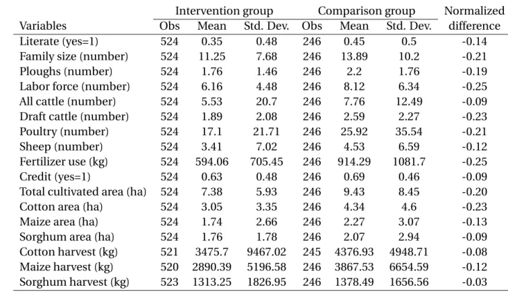
Table 1 reports mean values for various farmer characteristics collected during the baseline and final surveys. All normalized differences are below 0.25 standard deviations, which indicates that the randomization procedure was successful in constructing a valid control group (Imbens and Wooldridge, 2009). On average, treatment households are comprised of 11 members, 6 of whom are employed in farming activities; they own 7 hectares of land (9 ha on average in the control group) and devote about 20 percent of their land to maize, 20 percent to sorghum, and about 40 percent to cotton. Basic statistics on the main variables displayed in Table 2 suggest that attri-tion did not introduce important biases in the sample.

We compare our data with the nationally-representative agricultural survey carried out by the Burkina Faso Ministry of Agriculture in 2013 (Table 3). This survey includes 3,547 rural households that were randomly selected in each of the 45 provinces of Burkina Faso, among which 133 house-holds were located in the Tuy and Mouhoun provinces, where our project was implemented. Ta-ble 3 shows that average household characteristics are very similar between our sample and the households from the same geographic area that were included in the national survey. This sug-gests that, although we focused to some extent on CPF members for the study, our sample appears to be quite representative of households located in western Burkina Faso more broadly.

Participation in the system has been steadily increasing over the three seasons, reaching more

6_{Food security questions had no place in the 2013 survey, since it took place in January, long before the lean season.} 7_{In the survey, the farmer was asked: “How many days do you think your current stock will allow you to satisfy the}

than 30 percent in November 2015. This take up rate may seem low as compared to one other experimental project led in Burkina Faso that reached around 90 percent (Delavallade and God-lonton, 2020) and where the eligibility criterion was based on farmers willing to participate into the program whereas ours was based on farmers living in treated villages. In our study, eligible farmers were those living in treated villages, which includes those who were not willing to participate as well. Our final sample includes 180 farmers who participated in 2015 – and possibly during previ-ous years as well (Figure 3). As Table 4 shows, farmers electing to engage in a warrantage program stored a large portion of harvested crops – about 34 percent in 2015. The average number of bags stored per farmers declined over the years, which reflects the sucess of the device and the fact that village committees had to fix individual maximum amounts stored to ensure the participation of the greatest number given the 60 metrics tons storage capacity. Storage was comprised mainly of maize versus other staple food crops such as sorghum and millet. We find that the average amount of credit was higher in 2013 than in 2014 or 2015. This is mainly due to the fact that the proportion of those who chose to store without taking out a loan was also much lower in 2013 than in 2014 or 2015 revealing an higher commitment effect (Le Cotty et al., 2019).

4 Empirical strategy

We estimate a number of possible effects of warrantage, including economic decisions related to farming activities and food security. We first examine the impact of the program on households living in the villages where the program was implemented. Subsequently, we examine the impact of the program on households that actually used the warrantage device.

4.1 Parameters of interest

We first aim to estimate the intention-to-treat (ITT) parameter. This analysis includes every sub-ject who is randomized according to the randomized controlled trial, participant or not in the

warrantage system. The ITT is defined as ITT= E(y1− y0), where y1denotes the outcome level in

the presence of the program an y0denotes the outcome level in the absence of the program. In

the absence of spillover effects within treatment villages, it can be difficult to detect an effect of the program at the aggregate level, all the more so if that the participation rate is low and the ef-fects of the program on the participants are small. In our case, however, there is reason to believe that the warrantage system was able to benefit households other than those that actively partici-pated. First, farmers may have taken credit in their name for the purpose of sharing it with other households in informal arrangements. Typically, a farmer can store grain (and take credit in the process) on behalf of another farmer. This type of arrangement being informal, our data do not allow us to spot those "hidden" participants among those we designate as non-participants in our sample. Second, participants who became wealthier as a result of the warrantage system may have

decided to give their family and neighbours some of their earnings, typically in the form of dona-tions of grain during the lean season. One could thus expect the effect of the warrantage - if it exists - to be estimated through the ITT.

We then aim to estimate the average treatment effect on the treated (ATT) parameter, that is, the impact of the program on those households that actually used the warrantage scheme in 2015 (and possibly during previous years as well), which includes not only those who received credit but also those who chose to store without taking out a loan. This impact can be measured, for example, as the average quantity of grain still in stock in participants’ granaries at the lean season as a result of the project. It can also be, for example, the amount of land devoted to growing cotton on treated farms that is due to the program. To determine the quantity of grain quantity or area of land farmed, we need to calculate the difference between the outcome level as observed on participating farms in August 2016 and the outcome level that would have been observed in those farms at the same date, had they not been involved in warrantage. The ATT is defined as ATT=

E (y1− y0|D = 1), where y1denotes the outcome level in the presence of the program, y0denotes

the outcome level in the absence of the program, and D is a dummy variable which takes on the value of one when the farmer participated in the program and zero otherwise. We use various

approaches to estimate the outcome level in the unobserved state, namely E (y0|D = 1).

4.2 Estimators

We obtain an estimate of the ITT parameter by running a simple ordinary least squares (OLS) re-gression of the outcome y on treatment D, controlling for a set of pre-treatment covariates in the event that some imbalances remain across the treated and control groups despite the ran-domization procedure. In order to obtain an estimate of the ATT parameter, we turn to quasi-experimental approaches, which are both more tedious to implement and reliant on stronger hypotheses. The main concern when evaluating the effects of voluntary warrantage program arises from the fact that the participants in treatment communities self-selected into the pro-gram. To deal with this issue, we use the instrumental variable (IV) approach and the difference-in-difference (DID) matching approach.

We apply the IV estimator using the random allocation of the warrantage program as an in-strument. Note that in our setting where the only farmers who take the treatment (i.e. those who actually use the warrantage system) are those who were randomly assigned to be treated (i.e. they are offered access to the warrantage system), the IV estimator gives the ATT (Imbens and Rubin, 2015). We also use two DID-matching estimators as a robustness check: the 2-nearest-neighbour matching estimator, which matches each participant to the two closest untreated farmers from the control villages, according to the vector X and a propensity score method called inverse probabil-ity weighting (IPW) (Cattaneo, 2010). Matching eliminates selection bias due to observable fac-tors X by comparing treated farmers to observationally-identical untreated ones (Imbens, 2004).

The DID-matching estimator moreover allows for temporally invariant differences in outcomes between participants and their X -matched counterparts from the control villages. Applied to our data, this identification strategy consists of comparing the change in participants’ outcomes be-tween 2013 and 2016 with the change in outcomes among matched untreated farmers. We com-pute robust standard errors for matching estimators in a standard way. We moreover run a

stan-dard OLS regression with robust stanstan-dard errors adjusted for village clusters.8

In addition to the parallel trend assumption, DID-matching requires a selection on observ-ables assumption (Heckman and Robb, 1985), according to which the dependence between the treatment assignment and the treatment-specific outcomes can be entirely removed by condi-tioning on observable variables. To this end, a crucial step is thus to measure all factors X that are likely to drive both the decision to participate in the program as well as decisions regarding farming activities and food security. It is important that the observable factors X are not affected by the project (Imbens, 2004), which is why we use pre-treatment values from the baseline survey. We include in the set of observable factors X : the total cultivated land area (in hectares), the cot-ton area (in hectares), the maize area (in hectares), the sorghum area (in hectares), the amount of fertilizer used for maize (in kilograms), whether the farmer received a formal education, whether he received a credit during the previous year, the number of cattle, plows, and poultry the farmer owns, as well as the size of the farm’s labour force (measured as the number of family members who are employed in farming activities).

Another key assumption for the validity of both ITT and DID-matching approaches is that the treatment received by one farmer must not affect the outcome of another farmer located in one of the control villages. This assumption is referred to as the Stable-Unit-Treatment-Value-Assumption (Rubin, 1978). In our analysis, the validity of this assumption is not likely to be threat-ened because connections between villages are extremely limited due to the poor quality of trans-portation infrastructure. In addition, in the event that an individual from a control village requests permission to participate in the proposed scheme in the nearest treated village, he or she would be refused by the committee.

5 Results of the impact evaluation

5.1 ITT analysis

We first examine the impact of the treatment on a variety of outcomes for which we have collected data both in 2013 and 2016, which allows us to apply the fixed-effect estimator. These outcomes include the total cultivated land area (in hectares), the area under cotton farming (in hectares), the area under maize farming (in hectares), the area under sorghum farming (in hectares), the amount

8_{In addition to the assumption of linearity, using this estimator requires assuming that the impact of warrantage is}

of fertilizer used for maize (in kilograms), and the number of cattle, plows, poultry, and sheep. Table 5 displays the parameters estimates of a linear model that links the outcome and a dummy taking on the value of one when the farmer lives in a treatment village (and zero otherwise), as well as control variables (see Section 4.2). We find evidence that living in a treatment village improves farmers’ productive investment and capital accumulation.

First, farmers in treated villages after 3 years of warrantage cultivate in average a greater area (+1.8 ha, i.e. a 27% increase), devoted to cotton and maize cultivation. This result is in line with qualitative information collected in the field, which indicates that many participants chose to use their loan to hire farm workers to harvest more cotton (when they receive the credit). The main limiting factor of cotton cultivation in the Tuy and Mouhoun is not land availability but by liquidity constraint to hire daily workers for harvesting. Because the maize harvest takes place in October-November, the loan of warrantage comes in December which is the cotton harvesting period, and the warrantage actually alleviates this liquidity constraint, and favors cotton expansion.

Fertilizer use increase because maize and cotton are very closely related in Burkina Faso as . They subsequently apply part of the received fertilizers in their maize plots. Fertilizer utiliza-tion (NPK) on the farm increases indeed by an average of 160 kg (25%), mainly because cotton and maize production are closely related productions. Access to fertilizers is a side effect of cot-ton production because farmers receive chemical fertilizers from the parastatal cotcot-ton company during the planting season. Because cotton cultivation is a fully integrated production, the cot-ton company (Sofitex) provides producers with fertilizers for cotcot-ton and for maize (to minimize fertilizers diversion from cotton to maize cultivation). Furthermore, stock release at the end of warrantage creates a wealth effect that reduces liquidity constraint that benefits the purchase of inputs in general.

The cattle size increases in average by 1.5 head (38%). The mechanism of this important capital accumulation is also straightforward: a typical lean season for average householeds is a season of decapitalization after the grain stock is finished. The grain release at the beginning of the lean season simply mitigates the seasonal decapitalization.

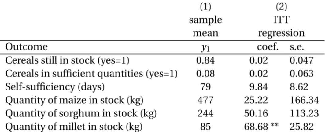
We then examine the impact of the treatment on a variety of outcomes for which we have collected data during the 2016 lean season (August). Table 6 displays the results, which suggest that living in a treatment village may have improved farmers’ food security, at least by increasing millet stock.

5.2 Project enrollment

The program was offered to all households living in treatment villages (including non-CPF mem-bers). Farmers were invited to participate in informational meetings and decided whether they would like to participate. This self-selection process might have led to a particular profile of partic-ipants that distinguishes them from those who never chose to participate in the scheme, whether

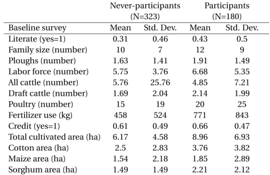
in 2013, 2014 or 2015 (Le Cotty et al., 2019). We thus begin our analysis by comparing participat-ing and non-participatparticipat-ing households livparticipat-ing in treatment villages (Figure 3). Table 7 shows that the subset of surveyed farmers who decided to participate in the warrantage system differ in some respects from farmers who did not. In particular, we find that participants have larger farms and larger areas of land under cotton farming. They also have larger families on average and are more likely to be literate. These features therefore play a central role in the matching procedure that follows.

5.3 Impacts on participants

Matching procedure

To estimate the ATT, we apply the aforementioned estimators to the group of participants, using those who were not offered the warrantage program to estimate the counterfactual level of out-comes (see Figure 3). This requires computing conditional probabilities for being enrolled in the

program (or propensity scores)9and for determining whether the matching procedure performed

well. Table 8 compares the extent of balancing between the participant and control groups before and after the matching procedure. All normalized differences are well below the suggested criteria of 0.25 standard deviations (Rubin, 2001; Imbens and Wooldridge, 2009), which indicates that the matching procedure was successful in constructing a valid control group.

Farming activities

Our estimates of the effects of warrantage on agricultural decisions among participants are pre-sented in Table 9. Column (1) gives the mean value of the outcome in 2016 among participants, while Columns (2)-(5) provide the impact of warrantage, that is, the difference between the value given in Column (1) and the estimated counterfactual value. For many outcomes, the impact is estimated with precision.

The impact on the total cultivated area varies from 1 ha (ipwr adjustment) to 2.41 ha (IV), the latter being probably the most robust estimate, and the most consistent with our ITT estimate. As the participants have an average of 10.5 hectares, the mean relative impact varies from 10 and 30 percent. Like the ITT, this impact on farmland is first of all due to an increase in cotton area, and then to an increase in maize area.

9_{We compute propensity scores for participants and controls by estimating a probit model, using the sample of}

par-ticipants and non-parpar-ticipants living in treatment villages (see Section 5.2), where the dependent variable is a dummy variable which takes on the value of one if the farmer is a participant (and zero otherwise). The explanatory variables include all of the pre-treatment covariates presented in Table 7. From the estimated parameters of this model, we then compute the conditional probabilities of participating in the program for both participants and controls. Fig-ure 4 shows that densities in both groups are high enough for a wide range of propensity scores, meaning that the matching procedure is likely to perform well.

The results also confirm that warrantage increased the area of land used to grow maize (as well as the quantity of fertilizer used for maize), albeit to a lesser extent (from less than half a hectare to 0.65 ha depending on the estimator).

The results moreover confirm that warrantage encouraged participating farmers to invest in productive assets, indicating that they used the loan (or the earnings generated through warran-tage during previous seasons) to buy cattle and sheep or to avoid selling them. This is a potential important impact because livestock can act as a buffer for consumption smoothing and also as an income generator.

This series of results suggests that warrantage (whether a loan with storage or storage alone) generated two types of effects: an increase in investment in factors of production (labor and land) whose returns will materialise as soon as the next harvest, and an increase in investment in pro-ductive assets that play a role as a financial safety net.

Food security

Table 10 displays the estimates of the impact of warrantage on various food security variables using the IV estimator, the matching estimators, and the OLS estimator. Column (1) again gives the mean value of the outcome in 2016 among participants on the common support, while Columns (2)-(5) provide the impact of warrantage, that is, the difference between the value given in Column (1) and the estimated value in the counterfactual scenario. Matching estimators produce statistically significant results for four outcomes: the probability of having grain in stock at the time of the sur-vey (+6 percentage points, taking the lowest estimate), the probability that the quantity of grain in stock is sufficient to satisfy basic consumption needs until the next harvest (+7 percentage points, taking the lowest estimate), the quantity of maize in stock (almost 200 kilograms, taking the lowest estimate), and finally the number of days of self-sufficiency (about 17 additional days).

However, we are able to provide significant results at standard levels of significance using the IV estimator for only one of these outcomes – the number of days of self-sufficiency. The mean value of this outcome among participants is 95 days and our estimates suggest that it would have been 78 days (95 − 17) in the absence of a warrantage system. These 17 additional days thus represent an increase of about 22 percent (17/78) in households’ ability to cope with the lean season, thanks to the warrantage scheme.

We next examine the diversity of the food consumed by households on a weekly basis. Table 11 displays the impact of warrantage on dietary diversity for the two outcomes for which we obtained statistically significant results, namely the probability of consuming the food several times a week and the probability of consuming the food daily. Results show that warrantage significantly in-creased the probability of consuming fish (+13 percentage points), oil (+9 percentage points), and fruit (+3 percentage points) several times a week. The results also indicate a significant increase in the probability of consuming fruit (+2 percentage points) and condiment (+9 percentage points)

on a daily basis.

6 Conclusion

Inventory credit systems have been celebrated for giving farmers access to credit and, in doing so, providing them with an opportunity to overcome the “sell low buy high” phenomenon, notably because providing access to credit enables farmers to adjust their selling activities throughout the year and take advantage of seasonal price fluctuations. In this paper, we quantified the effects of one of the first warrantage systems implemented in Burkina Faso. Our results suggest that such a system is likely to generate strong and long term effects on production, savings, and food security. As in many empirical studies, our findings are to some extent specific to the study area and/or the period analysed. As such, it is difficult to determine whether the effects we estimate can be generalized to other situations. For example, the long term on-the-ground presence of the project proponent – the CPF – and the trust that characterized the relationship between farmers, the CPF and the rural bank in the study areas probably contributed to such encouraging results. In a less favorable context, many households may have been reluctant to entrust their grain to a farmer or-ganization. It must also be recognized that the efficiency of the system can be significantly reduced when the state intervenes in the marketplace via price stabilization, as occurred in 2013.

We nevertheless believe there are several takeaways from our main findings. In particular, we show that warrantage is likely to increase investment in factors of production (labor and land) and in productive assets that also play a safety net role (cattle and sheep). We further provide evidence that warrantage can improve self-sufficiency by more than 20 percent and even improve dietary diversity by increasing the consumption of nutrient dense foods (fish, fruit, oil and condiments). Overall, these results suggest that warrantage is a promising development tool for African coun-tries.

Finally, additional investigations are needed to provide evidence of spillover effects within vil-lages and to show which of the two features of the system (access to credit or access to storage or a combination of both) has led to the effects we estimated. We keep this for future research.

Acknowledgments

This research would not have been possible without the full cooperation of the Confederation Paysanne du Faso. Funding for this research was provided by the European Union with addi-tional funding from AGRINATURA for the Farm Risk Management for Africa project, coordinated by CIRAD.

References

Aggarwal, S., Francis, E. and Robinson, J. (2018) Grain today, gain tomorrow: Evidence from a storage experiment with savings clubs in kenya, Journal of Development Economics, 134, 1 – 15. Ashraf, N., Karlan, D. and Yin, W. (2006) Tying odysseus to the mast: Evidence from a commitment

savings product in the philippines, Quarterly Journal of Economics, 121, 635–672.

Baland, J.-M., Guirkinger, C. and Mali, C. (2011) Pretending to be poor: Borrowing to escape forced solidarity in cameroon, Economic Development and Cultural Change, 60, 1 – 16.

Barr, A. and Genicot, G. (2008) Risk sharing, commitment, and information: An experimental anal-ysis, Journal of the European Economic Association, 6, 1151–1185.

Basu, K. and Wong, M. (2015) Evaluating seasonal food storage and credit programs in east in-donesia, Journal of Development Economics, 115, 200 – 216.

Bauer, M., Chytilova, J. and Morduch, J. (2012) Behavioral foundations of microcredit: Experimen-tal and survey evidence from rural india, American Economic Review, 102, 1118–39.

Beaman, L., Karlan, D. and Thuysbaert, B. (2014) Saving for a (not so) rainy day: A randomized evaluation of savings groups in mali, Working Paper 20600, National Bureau of Economic Re-search.

Burke, M., Bergquist, L. F. and Miguel, E. (2018) Sell Low and Buy High: Arbitrage and Local Price Effects in Kenyan Markets, The Quarterly Journal of Economics, 134, 785–842.

Casaburi, L., Glennerster, R., Suri, T. and Kamara, S. (2014) Providing collateral and improving product market access for smallholder farmers. a randomised evaluation of inventory credit in sierra leone, 3ie Impact Evaluation Report, 14.

Cattaneo, M. D. (2010) Efficient semiparametric estimation of multi-valued treatment effects un-der ignorability, Journal of Econometrics, 155, 138 – 154.

Coulter, J. and Onumah, G. (2002) The role of warehouse receipt systems in enhanced commodity marketing and rural livelihoods in africa, Food Policy, 27, 319 – 337.

Delavallade, C. A. and Godlonton, S. (2020) Locking crops to unlock investment: Experimental evidence on warrantage in burkina faso, World Bank Policy Research Working Paper.

di Falco, S. and Bulte, E. (2011) A dark side of social capital? kinship, consumption, and savings,

The Journal of Development Studies, 47, 1128–1151.

Dillon, B. M. (2017) Selling crops early to pay for school: A large-scale natural experiment in malawi, Tech. rep., SSRN Working Paper.

Fink, G., Jack, B. K. and Masiye, F. (2014) Seasonal credit constraints and agricultural labor supply: Evidence from zambia, Working Paper 20218, National Bureau of Economic Research.

Goldberg, J. (2017) The effect of social pressure on expenditures in malawi, Journal of Economic

Heckman, J. J. and Robb, R. (1985) Alternative methods for evaluating the impact of interventions: An overview, Journal of Econometrics, 30, 239 – 267.

Imbens, G. W. (2004) Nonparametric estimation of average treatment effects under exogeneity: A review, Review of Economics and statistics, 86, 4–29.

Imbens, G. W. and Rubin, D. B. (2015) Causal Inference for Statistics, Social, and Biomedical

Sci-ences: An Introduction, Cambridge University Press.

Imbens, G. W. and Wooldridge, J. M. (2009) Recent developments in the econometrics of program evaluation, Journal of economic literature, 47, 5–86.

Jakiela, P. and Ozier, O. (2015) Does Africa Need a Rotten Kin Theorem? Experimental Evidence from Village Economies, The Review of Economic Studies, 83, 231–268.

Kumar, D. and Kalita, P. (2017) Reducing postharvest losses during storage of grain crops to strengthen food security in developing countries, Foods, 6.

Le Cotty, T., Ma�tre d’H�tel, E., Soubeyran, R. and Subervie, J. (2019) Inventory Credit as a Commitment Device to Save Grain Until the Hunger Season, American Journal of Agricultural

Economics, 101, 1115–1139.

Ouattara, B., Taonda, S. J. B., Traoré, A., Sermé, I., Lompo, F., Peak, D., Sédogo, M. P. and Bationo, A. (2018) Use of a warrantage system to face rural poverty and hunger in the semi-arid area of burkina faso, Journal of Development and Agricultural Economics, 10, 55–63.

Pender, J., Abdoulaye, T., Ndjeunga, J., Gerard, B. and Kato, E. (2008) Impacts of inventory credit, input supply shops, and fertilizer microdosing in the drylands of niger, Tech. rep., IFPRI Discus-sion Paper.

Platteau, J.-P. (2000) Institutions, Social Norms and Economic Development, Harwood Academic Publishers, Amsterdam.

Rubin, D. B. (1978) Bayesian inference for causal effects: The role of randomization, The Annals of

statistics, 6, 34–58.

Rubin, D. B. (2001) Using propensity scores to help design observational studies: Application to the tobacco litigation, Health Services and Outcomes Research Methodology, 2, 169–188.

Stephens, E. C. and Barrett, C. B. (2011) Incomplete Credit Markets and Commodity Marketing Behaviour, Journal of Agricultural Economics, 62, 1–24.

Tabo, R., Bationo, A., Amadou, B., Marchal, D., Lompo, F., Gandah, M., Hassane, O., Diallo, M. K., Ndjeunga, J., Fatondji, D. et al. (2011) Fertilizer microdosing and warrantage or inventory credit system to improve food security and farmers income in west africa, in Innovations as key to the

7 Figures and Tables

Figure 2: Agricultural Activities and Warrantage Calendar

June July August Sept Oct Nov Dec January to April May Grain production Tilling Sowing Fertilizing Plant growing Weeding Fertilizing Harvesting Cotton production Tilling Sowing Fertilizing Plant growing Weeding Fertilizing Harvesting Inventory Credit (or warrantage) Storage Credit delivery Credit repayment Collateral restitution

Notes: Grain production refers to production of maize, millet and sorghum.

Figure 3: Sample composition Total sample 770 Intervention 524 Comparison 246 Participant in 2015 180 Non-participant in 2015 344 Participant before 2015 97 Non-participant before 2015 83 Participant before 2015 21 Never-participant 323

Figure 4: Distribution of propensity scores by groups 0 1 2 3 0 1 2 3 0 .1 .2 .3 .4 .5 .6 .7 .8 .9 1 Comparison group Participant group Density kdensity ps D e n si ty Pr(particip) Graphs by sample_estim

Note: The participant groups includes the 180 households that actu-ally used the warrantage scheme. The comparison group includes the 246 households that were not offered to participate in the program.

Table 1: Household characteristics (Baseline survey)

Intervention group Comparison group Normalized

Variables Obs Mean Std. Dev. Obs Mean Std. Dev. difference

Literate (yes=1) 524 0.35 0.48 246 0.45 0.5 -0.14

Family size (number) 524 11.25 7.68 246 13.89 10.2 -0.21

Ploughs (number) 524 1.76 1.46 246 2.2 1.76 -0.19

Labor force (number) 524 6.16 4.48 246 8.12 6.34 -0.25

All cattle (number) 524 5.53 20.7 246 7.76 12.49 -0.09

Draft cattle (number) 524 1.89 2.08 246 2.59 2.27 -0.23

Poultry (number) 524 17.1 21.71 246 25.92 35.54 -0.21

Sheep (number) 524 3.41 7.02 246 4.53 6.59 -0.12

Fertilizer use (kg) 524 594.06 705.45 246 914.29 1081.7 -0.25

Credit (yes=1) 524 0.63 0.48 246 0.69 0.46 -0.09

Total cultivated area (ha) 524 7.38 5.93 246 9.43 8.45 -0.20

Cotton area (ha) 524 3.05 3.35 246 4.34 4.6 -0.23

Maize area (ha) 524 1.74 2.66 246 2.27 3.07 -0.13

Sorghum area (ha) 524 1.76 1.78 246 2.07 2.94 -0.09

Cotton harvest (kg) 521 3475.7 9467.02 245 4376.93 4948.71 -0.08

Maize harvest (kg) 520 2890.39 5196.58 246 3867.53 6654.59 -0.12

Sorghum harvest (kg) 523 1313.25 1826.95 246 1378.49 1656.56 -0.03

Note: Intervention group refers to the households living in the villages where the warehouses were built in 2013. Comparison group refers to the households living in the villages that were not offered to participate in the project. The normalized difference is the difference in means divided by the square root of the sum of variances for both groups.

T a bl e 2: S u rv ey at tr it io n Initial samp le (N=93 3) F in al sample (N = 7 70 ) T reat ed C ont rols T reat ed C ont rols B a se line sur v ey O bs M e a n S.D . Ob s M ean S .D Ob s M ean S.D . Obs M ean S.D . T ot al cu lt iv a ted ar ea (ha) 68 1 7.2 5 .8 25 2 9 .5 8 .6 52 4 7.4 5.9 24 6 9 .4 8 .5 C ot ton a rea (h a) 68 1 3.1 3 .4 25 2 4 .3 4 .6 52 4 3 3.4 24 6 4 .3 4 .6 M ai ze ar ea (ha ) 68 1 1.5 2 .4 25 2 2 .3 3 .1 52 4 1.7 2.7 24 6 2 .3 3 .1 S or gh u m a rea (h a) 68 1 1.8 1 .7 25 2 2 .1 3 .1 52 4 1.8 1.8 24 6 2 .1 2 .9 All cat tle (number) 68 1 5.5 19 25 2 7 .9 1 2.6 52 4 5.5 2 0.7 24 6 7 .8 1 2.5 D raf t c at tle (number) 68 1 1.8 2 25 2 2 .6 2 .4 52 4 1.9 2.1 24 6 2 .6 2 .3 P oul tr y (number) 68 1 1 6. 4 2 0.9 25 2 26 .1 3 5.5 52 4 17. 1 2 1.7 24 6 2 5.9 3 5.5 N ote: T re a ted gr ou p refers to th e hou se h ol d s liv in g in th e v ill ag es w h er e th e war eh ou ses w er e bui lt in 20 13. C ont rol g rou p refers to the h o useholds li ving in the vi llages that w er e not off er ed to par ticipat e in th e p roj ec t. T he main c au se of at tr it io n is d u e to th e decisio n of one vi llage in the c o n tr ol g rou p to leav e th e pr o g ra m and not to par ticipa te in the fin al su rv ey in 20 16 .

Table 3: Representativeness of the sample

Sample National survey

(N=770) (N=133)

Baseline survey Mean Std. Dev. Mean Std. Dev.

Total cultivated area (ha) 8.04 6.9 6.98 6.98

Cotton area (ha) 3.46 3.84 3.61 4.71

Maize area (ha) 1.91 2.81 1.82 2.04

Sorghum area (ha) 1.86 2.22 1.98 2.29

Draft cattle (number) 2.11 2.16 3.05 4.62

Family size (number) 12.10 8.65 10.58 6.29

Note: This table displays summary statistics for main characteristics of farmers. The second column displays an extraction from a national agricul-tural survey led in 2013 by the Ministry of Agriculture of Burkina Faso. This sample is representative of the Tuy and Mouhoun regions.

Table 4: Participation in warrantage: summary statistics

Characteristics 2013 2014 2015

Number of farmers 60 105 180

Adoption rate 0.11 0.20 0.34

Average nb of maize bags stored 14.5 11.5 10.4

Average nb of sorghum bags stored 2.2 1.3 1.0

Average nb of millet bags stored 0.8 0.5 0.3

Average share of harvest stored (%) 0.28 0.23 0.34

Table 5: Impact on farming activities: ITT estimates

(1) (2) sample ITT

mean regression Outcome y1 coef. s.e.

Total cultivated area (ha) 8.56 1.82 *** 0.54 Cotton area (ha) 4.16 1.22 * 0.58 Maize area (ha) 2.09 0.46 *** 0.14 Sorghum area (ha) 1.58 0.32 0.22 All cattle (number) 5.63 1.57 ** 0.71 Draft cattle (number) 2.01 -0.3 0.20 Poultry (number) 14.36 -2.12 3.41 Sheep (number) 3.8 0.87 0.82 Fertilizer use (kg) 811 163.05 ** 76.49 Cotton harvest (kg) 3,758 721.58 * 379.09 Maize harvest (kg) 2,947 -11.31 214.64 Sorghum harvest (kg) 1,039 -156.38 208.49

Note: This table presents the ITT estimates. Column 1 gives the mean value of the outcome level (y1) amongst treated households in 2016.

Column 2 gives the ITT using an OLS regression that includes a set of covariates as controls: the total cultivated area (in ha), the cotton area (in ha), the maize area (in ha), the sorghum area (in ha), the education level of the head of the family (literate=1), the family size (number), the number of ploughs, the labor force (number of active members), the cattle (number), the draft cattle (number), poultry (number), fer-tilizer use (in kg), credit access (yes=1) and the existence of another warehouse in the village (yes=1). Robust standard errors are adjusted for village clusters.The ***, ** and * indicate that the estimated co-efficients are statistically significant at the 1%, 5%, and 10% levels, respectively

Table 6: Impact on access to sufficient food: ITT estimates

(1) (2)

sample ITT

mean regression

Outcome y1 coef. s.e.

Cereals still in stock (yes=1) 0.84 0.02 0.047

Cereals in sufficient quantities (yes=1) 0.08 0.02 0.063

Self-sufficiency (days) 79 9.84 8.62

Quantity of maize in stock (kg) 477 25.22 166.34

Quantity of sorghum in stock (kg) 244 50.16 113.23

Quantity of millet in stock (kg) 85 68.68 ** 25.82

Note: This table presents the ITT estimates. Column 1 gives the mean value of the outcome level (y1) amongst treated households in 2016. Column 2 gives the

ITT using an OLS regression that includes a set of covariates as controls: the total cultivated area (in ha), the cotton area (in ha), the maize area (in ha), the sorghum area (in ha), the education level of the head of the family (literate=1), the family size (number), the number of ploughs, the labor force (number of active members), the cattle (number), the draft cattle (number), poultry (number), fertilizer use (in kg), credit access (yes=1) and the existence of another warehouse in the village (yes=1). Robust standard errors are adjusted for village clusters. The ** indicate that the estimated coefficients are statistically significant at the 5% level

Table 7: Participants vs Never-participants: Summary statistics

Never-participants Participants

(N=323) (N=180)

Baseline survey Mean Std. Dev. Mean Std. Dev.

Literate (yes=1) 0.31 0.46 0.43 0.5

Family size (number) 10 7 12 9

Ploughs (number) 1.63 1.41 1.91 1.49

Labor force (number) 5.75 3.76 6.68 5.35

All cattle (number) 5.76 25.76 4.85 7.21

Draft cattle (number) 1.69 2.04 2.14 1.99

Poultry (number) 15 19 20 25

Fertilizer use (kg) 458 524 771 843

Credit (yes=1) 0.61 0.49 0.66 0.47

Total cultivated area (ha) 6.17 4.58 8.96 6.93

Cotton area (ha) 2.5 2.83 3.76 3.82

Maize area (ha) 1.54 2.18 1.85 2.89

Sorghum area (ha) 1.49 1.49 2.21 2.12

Note: Participants are the households living in the villages where the warehouses were built in 2013, who actually used the warrantage scheme in 2015 and possibly in the years before. Never-participants refer to the households living in the villages where the warehouses were built in 2013, who decided not to use the warrantage scheme (neither in 2015 nor before).

T a bl e 8: B al a ncin g te sts bef or e an d aft er mat chin g V ar iab les in 201 3 T reat e d C ont rol (i p wr a) C ont rol (2-nn ) S D bef o re ip wr a S D af ter ip wr a SD bef or e 2 n n S D af ter 2nn T ot al lan d ar e a (ha) 10 .9 1 0.1 9. 8 -0.1 0 -0 .01 -0.1 4 -0 .04 C ot ton a rea (h a) 4. 3 3 .8 3. 7 -0.1 4 0. 00 -0.1 6 0. 01 M a iz e ar ea (ha ) 2. 3 1 .8 1. 9 -0.1 4 -0 .01 -0.1 3 -0 .03 S o rgh u m a rea (h a) 2. 1 2 .2 2. 1 0.0 5 -0 .05 0.0 0 -0 .07 L it er at e (y es=1) 0. 5 0 .4 0. 4 -0.0 4 -0 .02 -0.0 2 -0 .14 F a mi ly si ze (n u mb er ) 13 .9 1 2.5 11 .8 -0.1 5 0. 00 -0.2 3 -0 .07 P lou g hs (n u m ber) 2. 2 1 .9 1. 9 -0.1 8 -0 .03 -0.1 9 -0 .01 L a bor for c e (number) 8. 1 6 .7 6. 7 -0.2 4 -0 .03 -0.2 5 -0 .08 All c at tle (number) 7. 8 4 .9 4. 5 -0.2 9 -0 .02 -0.3 2 -0 .05 D raf t c att le (number) 2. 6 2 .1 2. 1 -0.2 1 -0 .03 -0.2 4 -0 .01 P oul tr y (number) 25 .9 1 9.8 20 .0 -0.2 0 -0 .02 -0.1 9 0. 02 F er til iz er u se (kg ) 9 14 .3 77 0. 7 7 54 .5 -0.1 5 0. 01 -0.1 6 0. 00 C redit (y es= 1 ) 0. 7 0 .7 0. 7 -0.0 6 -0 .01 -0.0 4 0. 02 N ote: This ta bl e pr o v ides mean v alue s of pr e-tr eat ment c o v ar iat es in bot h tr eated and con tr ol gr o ups as cons tr uct ed using the 2-nn an d th e ip wr a est im ators . It mor eo v e r pr o vi d e s the stan dar diz ed diff er e n ce (S D) in means the two gr ou ps . SD in mean s is con sider ed neg ligible when it is bel o w th e sugg e sted ru le o f thumb of 0. 25 stan dar d dev iat io n s(R ubin, 20 01 ; Imbens andW ooldr idg e , 2 00 9).

T a bl e 9: Impac t on par ticipan ts ’ far m in g ac tivi tie s (1) (2) (3) (4) (5 ) samp le 2 -n e a rest -n ei g hbor ip wr OL S IV mean m atc hing adju st ment regr essio n regr essio n D epen dent v ar iab le y1 coef . s.e . c o ef . s.e . coef. s.e . coef . s.e . T ot al cu lt iv a ted ar ea (ha) 10 .7 1 1.5 1 ** 0. 68 1. 00 * 0. 54 1. 36 ** 0. 64 2. 41 ** 1. 04 C ot ton a rea (h a) 5 .57 1.4 5 *** 0. 47 1. 17 *** 0. 35 1. 29 ** 0. 51 1. 70 *** 0. 62 M a iz e ar ea (ha ) 2 .41 0.3 5 * 0. 21 0. 28 ** 0. 14 0. 28 * 0. 14 0. 65 ** 0. 33 S o rgh u m a rea (h a) 1 .78 -0.1 2 0. 22 -0 .07 0. 22 0. 06 0. 26 0. 82 * 0. 44 All cat tle (number) 6 .33 1.4 3 ¦ 0. 91 1. 39 ** 0. 65 1. 54 ** 0. 66 2. 71 * 1. 42 D raf t c at tle (number) 2 .53 0.0 7 0. 21 0. 07 0. 17 0. 09 0. 21 -0 .39 0. 32 P oul tr y (number) 18 .4 3 2.2 8 2. 78 0. 05 2. 22 0. 70 3. 04 -3 .96 4. 78 S heep (n u mb e r) 4 .50 0.4 4 0. 52 1. 18 ** 0. 50 1. 15 ** 0. 48 1.3 6 1. 05 F er til iz er u se (k g) 112 5. 28 19 2.9 9 ** 76 .3 3 18 9. 14 *** 58 .8 8 20 2. 09 ** 77 .6 7 23 0.0 4 ** 11 7.2 0 C ot ton h ar v e st (kg ) 532 1. 49 82 7.9 5 * 43 0. 22 75 4. 25 ** 33 6. 20 91 3. 68 ¦ 54 8. 41 78 1.6 5 66 4.5 6 M a iz e h ar v est (kg) 373 2. 01 47 4.3 2 ¦ 32 4. 81 47 6. 93 * 25 2. 65 52 9. 51 32 8. 86 32 1.9 5 60 7.3 0 S o rgh u m h ar v e st (kg ) 121 9. 51 -15 3.5 1 17 8. 10 -1 32 .00 15 8. 74 -1 42 .85 29 6. 42 -1 77 .05 33 0.7 7 N ote: Th is tab le p resent s the est im ates using th e D ID a ppr oach . C o lumn 1 g iv es the m e a n v a lue of the outcome lev el (y1 ) amon gst tr eat e d househol d s in 2 01 6. C ol umn 2 giv es the A T T u sing the 2-near est-neigh bor est ima tor ,along wi th th e robust st anda rd-err or est ima tor p ro vided b y A b adie an d Imben s (20 06 , 20 11 , 20 12). C olu m n 3 giv es th e A T T u sin g th e in v e rse-pr obabil it y-w eigh ted reg ression adju stmen t (ip wr a) est imat o r, along wi th ro b u st st an dar d err ors . C olu mn 4 giv es the A T T u si n g an or d in ar y least sq uar es (ol s) re g ression, alo n g wi th robust st anda rd err ors a dj usted fo r vi llage clu st ers . C ol umn 5 giv es the A T T u sin g an inst ru m ent al v ar iable (IV ) regr e ssi on tak in g the (r an dom) loc ation of w ar ehouses as an inst ru m ent for par ticipa tion in warr ant age , along w ith ro b u st sta nda rd err ors . Th e ***, **, * a nd ¦ indica te that the est ima ted c oe ffi cien ts a re st atist ic all y sign ifi can t at the 1%, 5 %, 10% and 1 5% lev el s, resp ect iv ely .

T a bl e 10 : Im pact on p ar ti c ip ant s’ ac cess to su ffi cient food (1) (2 ) (3) (4) (5) samp le 2-near e st-neigh bor ip w r mean mat ch in g adju stmen t OLS IV D epen dent v ar iab le y1 coef . s.e . coef. s.e . c o ef . s.e . coef. s.e . C er e a ls st il l in st ock (y es= 1 ) 0. 94 0 .09 ** 0. 04 0. 06 ** 0. 03 0. 05 (a) 0. 01 (a) C er e a ls st or ed in su ffi cient qu an tities (y es= 1 ) 0. 81 0 .13 *** 0. 05 0. 07 * 0. 04 0. 06 (a) 0. 03 (a) S el f-suffi ciency (days) 95 .4 1 7.4 *** 6. 6 17 .7 *** 5. 6 17 .1 * 8. 5 21 .3 * 11 .5 Q u an tity of ma iz e in stock (kg ) 74 6.0 21 3.2 ** 10 1. 5 19 7. 6 * 10 4.1 21 6. 5 17 8. 0 58 .1 21 3. 8 Q u an tity of sor gh u m in stock (kg ) 31 8.8 -16 7.7 20 9. 8 -9 8.6 12 5.2 -7 1. 6 20 5. 3 -6 8. 9 15 2. 8 Q u an tity of mill et in st ock (kg) 94 .81 3 4.2 51 .9 42 .1 49 .1 33 .6 47 .6 13 0. 8 79 .7 N ote: C olu m n 1 g iv es th e mean v alu e of the ou tcome lev el (y1 ) am o n gs t tr eat ed h o useholds in 2 016 . C o lumn 2 g iv e s th e A T T u sin g the 2-near est-neigh bor esti-mat or , along with th e robu st st and ar d-err or estimat or pr o v ided b y A bad ie an d Imbens (200 6, 20 11 , 20 12 ). C ol umn 3 g iv es the A T T u sin g the inv erse-pr oba bi lity -w eight ed regr essio n adj ust ment (ip w ra) e stimat or , a lon g w ith robu st stan dar d err ors . C olu mn 4 g iv es the A T T u sin g an or din ar y least squ ar es (ols) regr essio n , along wi th ro b u st stan dar d err o rs adju sted for v ill a ge clu st er s. C ol umn 5 giv es th e A T T using a n in st ru m e n ta l v ar iab le (IV ) re g ression taking the (r andom) loca-tion of war eh ou ses as an in str u men t for par ticipat ion in w arr an tag e , al on g wi th robust st an dar d err ors . (a ) F or bin ar y d e p enden t v ar iab les , C ol umns (4) and (5) pr o vi d e th e mar g inal eff ect calculated fr om a pr o b it model (in those c ases , stan dar d err ors ar e not pr o vi ded). T he ***, **, * an d ¦ indica te that the est im ated coeffi cient s ar e st at ist ically sign ifi can t at th e 1 %, 5%, 10% and 15% lev els , respect iv el y.