HAL Id: hal-01522809
https://hal.archives-ouvertes.fr/hal-01522809
Submitted on 15 May 2017
HAL is a multi-disciplinary open access
archive for the deposit and dissemination of
sci-entific research documents, whether they are
pub-lished or not. The documents may come from
teaching and research institutions in France or
abroad, or from public or private research centers.
L’archive ouverte pluridisciplinaire HAL, est
destinée au dépôt et à la diffusion de documents
scientifiques de niveau recherche, publiés ou non,
émanant des établissements d’enseignement et de
recherche français ou étrangers, des laboratoires
publics ou privés.
Using scattered hyperspectral imagery data to map the
soil properties of a region
Philippe Lagacherie, Jean-Stéphane Bailly, P. Monestiez, Cecile Gomez
To cite this version:
Philippe Lagacherie, Jean-Stéphane Bailly, P. Monestiez, Cecile Gomez. Using scattered hyperspectral
imagery data to map the soil properties of a region. European Journal of Soil Science, Wiley, 2012,
63 (1), pp.110-119. �10.1111/j.1365-2389.2011.01409.x�. �hal-01522809�
Using scattered hyperspectral imagery data to map
the soil properties of a region
P . L a g a c h e r i e a , J . S . B a i l l y b , P . M o n e s t i e z c & C . G o m e z d
a INRA Laboratoire d’e´tude des Interaction Sol Agrosyste`me Hydrosyste`me (LISAH), Campus de la Gaillarde, 2 place Viala, 34060 Montpellier, France, b AgroParisTech Laboratoire d’e´tude des Interaction Sol Agrosyste`me Hydrosyste`me (LISAH), Campus de la Gaillarde, 2 place Viala, 34060 Montpellier, France, c INRA Unite´ Biostatistique et Processus Spatiaux (BioSP), Domaine Saint Paul, Site Agroparc, 84914 Avignon, cedex 9, France, and d IRD Laboratoire d’e´tude des Interaction Sol Agrosyste`me Hydrosyste`me (LISAH), Campus de la Gaillarde, 2 place Viala, 34060 Montpellier, France
Introduction
Given the relative lack of, and huge demand for, quantitative spa- tial soil information to be used in environmental management and modelling, digital soil mapping (DSM) has been proposed as an alternative to classical soil surveys for the quantitative mapping of soil properties over regions at intermediate (20 – 200 m) spatial resolutions (McBratney et al., 2003). A DSM program aiming to map soil properties at global level with a 3 arc second spatial resolution has been recently launched (Sanchez et al., 2009).
McBratney et al. (2003) proposed the equation S = f(s, c, o, r, p, a, n) for summarizing the general principle of DSM. According to this equation, a soil type or a soil property (S) can be predicted by a spatial inference function (f) using, as input, the existing soil information (s), the spatial covariates that map the different factors of soil formation, as defined by Jenny (1941) (c, o, r, p, a,), and the geographical location (n), which can capture any
Correspondence: P. Lagacherie. E-mail: lagache@supagro.inra.fr Received 4 October 2010; revised version accepted 28 September 2011
spatial trends missed by the other covariates. There has been a growing interest in using soil sensing technologies in DSM studies as a way to document s (Grunwald, 2009). However, these technologies have more often been used to complement analytical soil data for individual site characterization than to produce spatial inputs of DSM models and their applications at landscape scale are even more scarce (Grunwald, 2009). Recent progress in the development of these soil sensing techniques (Ben-Dor et al., 2008; Viscarra Rossel et al., 2010), leads us to anticipate their extensive application in DSM in the near future.
Among the available soil sensors, visible near infrared (Vis- NIR) imaging spectrometry looks to be one of the most promising. In laboratory studies, the capability of Vis-NIR spectroscopy (450 – 250 nm) to accurately quantify soil property contents has been already proven (Viscarra Rossel et al., 2006). More recently, spatial predictions of some usual soil properties for bare soil surfaces were obtained from high-resolution airborne hyperspectral images with uncertainties ranging from R2 = 0.53 to 0.75 depending on the study areas and their properties (Selige
et al., 2006; Gomez et al., 2008; Lagacherie et al., 2008; Stevens
MONTPELLIER
et al., 2010; Schwanghart & Jarmer, 2011). Although these results revealed a decrease in precision because of atmospheric effects and the signal to noise ratio (SNR) of the instrument (Lagacherie et al., 2008), imaging spectrometry provided correlations with soil properties of bare surfaces that out-performed most of the soil covariates usually considered in DSM applications. This present paper examines how this new input can be used for the DSM of
soil properties over large spatial areas. PEZENAS
Airborne Vis-NIR imaging spectrometry differs greatly in spatial resolution and extent from those currently handled in DSM. Airborne Vis-Nir sensors provide data at very fine spatial resolutions, including less than 5 m, which is much finer than the resolutions of the usual spatial covariates and target resolutions of DSM (see above). Also, the applications of imaging spectrometry are limited in space because of clouds and vegetation that mask the soil surface. These disruptions can result in scattered spatial data with isolated measured areas separated by non-measured areas.
To overcome these problems, we propose and test the block- co-kriging of clay content at different spatial resolutions using, as a covariate, a clay content indicator derived from an airborne hyperspectral sensor. The mapping was carried out over a 24.6-km2 area located in the vineyard plain of Languedoc with usable hyperspectral data scattered over only 3.5% of this area.
The case study
Study area
The study was carried out in the La Peyne catchment (Figure 1) in the south of France (43◦ 29 N and 3◦ 22 E). Vineyards form the primary land-use in the area. Marl, limestone and calcareous sand- stones from Miocene marine and lacustrine sediments formed the parent material of several soil types observed in this area, includ- ing Lithic Leptosols, Calcaric Regosols and Calcaric Cambisols (WRB soil classification, ISSS-ISRIC-FAO, 1998). These sedi- ments were partly covered by successive alluvial deposits ranging from the Pliocene to Holocene and differing in their initial nature and in the duration of weathering conditions. These sediments have produced an intricate soil pattern that includes a large range of soil types, such as Calcaric, Chromic and Eutric Cambisols, Chromic and Eutric Luvisols and Eutric Fluvisols. The local trans- port of colluvial material along the slopes has added to the com- plexity of the soil patterns. An earlier ground sampling made in the study region (Lagacherie et al., 2008) showed that these complex soil patterns correspond to a great variability of clay content at the soil surface (from 65 to 452 g kg – 1 ). A study area of 24.6 km2 (Figure 1) was defined by intersecting this region of interest with the hyperspectral image used in this study (see below).
The data
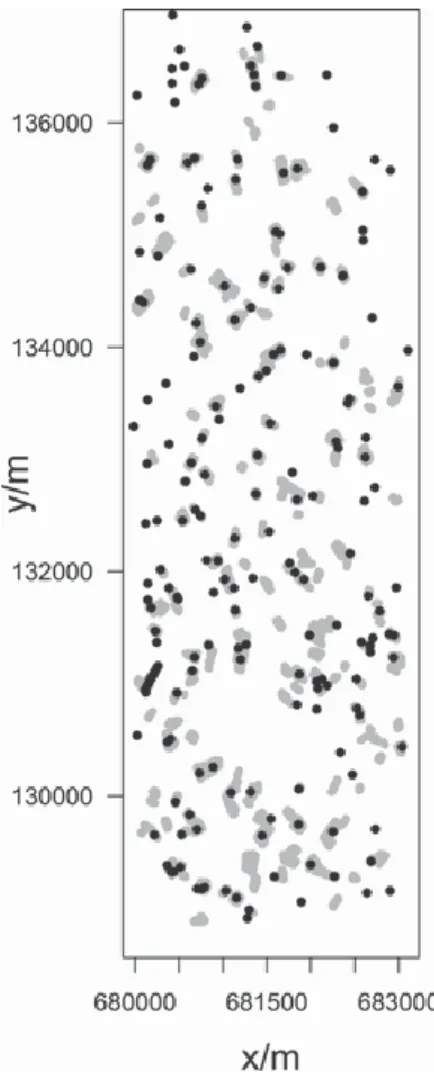
The dataset used in this study (Figure 2) included a set of 200 sites with measurements of the clay content (in g kg – 1 ) by means of a classical laboratory analysis (Robinson pipette) and a set
BEZIERS
Figure 1 Location of the study area (the grey rectangle).
Figure 2 The sites with measurements of clay content (black dots) and
the bare soil fields with estimations of clay content from the HYMAP data (grey areas).
of 192 bare soil fields with clay content estimations from a hyperspectral image that together covered 84.8 ha (3.5%) of the study area. These two types of data are successively described in
i j =
One hundred and thirty-seven sites of the set of 200 were located in the bare soil fields and so clay content measurements and hyperspectral estimations were available for these. The remaining 63 sites were located in vineyard areas and had clay content measurements only because the presence of vegetation prevented us from obtaining hyperspectral estimates. All of these samples were composed of five subsamples collected to a depth of 5 cm and representing, at best, a 5-m-wide square centred on the geographical position recorded by a decimetric GPS instrument. After homogenization of the sample and removal of plant debris and stones, about 20 g was used for analysis of soil properties. The initial samples were sieved and air-dried prior to transport to the laboratory for analysis.
The HYMAP airborne imaging spectrometer measured reflected radiance in 126 non-contiguous bands covering the 400 – 2500-nm spectral range with around 19-nm bandwidths and aver-
Methods
Modelling multivariate spatial correlations
In this study, the soil variable (here, clay content) and the soil sensing covariable (here, loglogCR2206 ) are denoted as Z1 and Z2 , respectively. Suppose that u is a location in two-dimensional space and Z1 (u) and Z2 (u) are spatial random functions. The random functions are assumed to satisfy the hypothesis of second-order stationarity (Matheron, 1971). Assuming that the soil variable (Z1 ) is spatially cross-correlated with the soil sensing covariable (Z2 ),
the spatial cross-correlation between Z1 and Z2 can be quantified by a cross-covariance function or a cross-variogram as defined in Wackernagel (1995). In univariate or bivariate frameworks, the covariance and variogram functions can be estimated as follows:
N (h )
age sampling intervals of 17 nm in the 1950 – 2480 nm domain
Cˆ z z (h) 1 (z (u ) z¯ )(z (u h ) z¯ ), (1)
(http://www.intspec.com/). The HYMAP image was acquired on 13 July 2003 from 3000-m altitude, providing a 5 × 5-m spa- tial resolution. Radiometric calibration was performed inflight (Richter, 1996) using nadir ground measurements (Beisl, 2001). The ATCOR4 code for airborne sensors was used for atmo-
i j and = N (h ) α=1 1 i α − i N (h ) j α + − j
spheric corrections (Richter & Schla¨pfer, 2000). Topographic cor- rections were performed with a high-resolution digital elevation
γˆ z z (h ) 2N (h ) α=1 (zi (u α + h ) − zi (u α )) model from the Institut Ge´ographique National (www.ign.fr) and
differential GPS (DGPS) ground control points.
The image was masked by using normalized difference vegetation index (NDVI) to remove living vegetation (essentially vineyards). The cellulose absorption band (2010 nm) was used to remove dry vegetation. Small areas of bare soils that could not be representative of neighbouring soil characteristics were also removed. Finally, the image provided usable data over 33,782 5 × 5 m pixels covering 3.5% of the total area only; that is, the bare soil fields that were randomly scattered over the region at the date of measurement.
In a previous study (Lagacherie et al., 2008), a continuum removal (CR) technique (Clark & Roush, 1984) was applied to HYMAP reflectance measurements to estimate clay contents. The clay contents were predicted from the depths of the absorption peaks at bands of 2206 nm (CR2206 ) that were computed as the differences between HYMAP reflectances and continua approximated by a straight line joining two local reflectance maxima placed on both shoulders of the peak absorption wavelength (see more details in Lagacherie et al., 2008). The prediction performances at local sites measured by cross-validation resulted in an R2 value of 0.58 and a root mean square error (RMSE) of 82 g kg – 1 . These prediction performances were similar to those of a 1:25 000 soil map in the same region (Leenhardt et al., 1994) while providing a much finer spatial resolution than a soil map at less cost. We therefore considered that CR2206 could be a suitable covariate to map clay content by DSM. To normalize the CR2206 distribution, a double log transformation was applied in further computations. This resulting variable will be denoted as loglogCR2206.
× (zj (u α + h ) − zj (u α )). (2)
In Equations (1) and (2), i and j belong to {1, 2}. When i = j , Equations (1) and (2) denote the usual covariance and variogram estimates. When i = j , Equations (1) and (2) denote the cross-covariance and cross-variogram estimates, respectively.
h is the separation vector between the data locations u α and
u α + h (the translation of h from u α ), zi (u α ) and zj (uα + h)
are observations of the variable zi and zj at spatial locations u α
and u α + h, respectively, z¯i and z¯j are arithmetic means of zi
and zj , respectively, and N (h ) is the number of distinct pairs
of observations at distance h . In the bivariate case (i = j ), these two expressions still have a known relationship (Wackernagel, 1995). They convey the same amount of information only if the cross-covariances are even functions. In this latter case, cross-variogram expressions are preferred for convenience, as in univariate frameworks.
To undertake the co-kriging (see later), a variogram matrix in which the diagonal entries are variograms and the off-diagonal entries are cross-variograms must be strictly conditionally negative definite. To ensure this condition, intrinsic or linear co-regionalization models can be used. The formulation of the latter in the bivariate case with two nested spatial structures is (Wackernagel, 1995)
(h ) = B1 g1(h ) + B2 g2(h ) , (3) where g1 (h) and g2 (h) are two normalized variograms, one for each spatial structure, and B 1 and B 2 are positive semi-definite 2 × 2 matrices.
σ 2 1
α α
σ 2
Co-kriging
The co-kriging estimator is a best linear unbiased estimator (BLUE) and has minimum estimation error variance (Wacker- nagel, 1995). In the two variable case, the ordinary co-kriging estimator is a linear combination of weights w1 and w2 with data
where γz1 z1 (v(u ), v(u )) is the mean within block semi-variance and it is approximated by the arithmetic average of the variogram between any two discretised points within the block v(u ). To simplify the notation, it is further denoted γ¯ (v, v). Then,
γz1 zj (u α , v(u )) is the variogram (j = 1) or cross-variogram
α α
(j = 2) between the data support uα and the block v(u ), and it is from the two variables Z1 and Z2 located at sample points in the
neighbourhood of a spatial location u0 . Each variable is defined with a set of samples of possibly different sizes n1 and n2 , and the estimator is defined as:
n1 n2
approximated by the arithmetic average of the variogram between the data support and the points discretising the block v(u ).
Validation procedure Z1 (u 0 ) = w1 Z1 (u α ) + w2 Z2 (u α ), (4) α α=1 α
α=1 A true validation of the above procedure would ideally require
where the weights w1 α α and w2 are solutions of a co-kriging system us to collect composite soil samples to estimate the within-pixel mean values of the soil property over a sufficient number of loca-and sum to 1 loca-and 0, respectively.
tions to represent the variations of these mean values satisfactorily The co-kriging variance of the estimation error of Z1 in the two
variables case can be estimated from the variogram γz1 z1 and the cross-variogram γz1 z2 (Wackernagel, 1995) by using the following expression
over the study area. A single composite soil sample requires several initial samples; for example, 25 initial samples for the 20 × 20 m sites of the French National Soil Quality Monitoring Network (Jolivet et al., 2006). Thus several hundred initial
sam-E (u 0 ) = n1 n2 wα γz z (u α − u ) + w2 γz z (u α − u ) + μz1 ,
ples would have to be collected for validation only, which would lead to sampling densities that are rarely possible in DSM studies. 1 1
α=1 0 α=1 α 1 2 0
(5) An alternative to this purely experimental validation method was therefore undertaken to verify that the approach provided a reason- able approximation of the ground truth. We first cross-validated the where μz1 is the Lagrange multiplier of the co-kriging system and
u α – u 0 denotes the distance between u α and u 0 locations.
Block co-kriging
The predictions of the soil property Z1 are required for the set of pixels (or square blocks) that are larger than the support of the input data. To obtain such predictions, it is possible to apply a block-ordinary co-kriging procedure (Gertner et al., 2007) that can combine and scale up the soil property measurements and the high-resolution sensing images available on a scattered set of fields. Let v(u ) denote a block centred at location u , n1 is the number of local measurements of the soil property, and n2 is the number of the soil sensing data from the images. The ordinary co-kriging estimator for the block v(u) is
n1 n2 Zˆ 1 (v(u )) = λ1 Z 1 (u α ) + λ2 Z 2 (u α ), (6)
co-regionalization model by applying an exact ordinary co-kriging and verifying that the co-kriging error variances were correctly predicted over the study area. We thus assume that correctly pre- dicted punctual co-kriging errors prevent incorrectly estimated model parameters, especially those for nugget values. With lim- itations from this assumed model parameter, we considered the block co-kriging error variances were correctly predicted over the study area.
Then we considered the block co-kriging error variances cal- culated from the same co-regionalization model as an estimator of the error on the mean value of the soil property. The val- idation of the ordinary co-kriging was done by comparing the true measurements with the predicted values obtained from a leave-one-out cross-validation. The error variance given by the co-regionalization model over the whole study area was first compared with the mean square error deduced from the
cross-α α=1
α
α=1 validation.
To evaluate more precisely if the model can predict the local where λ1 and λ2 are the weights of the block v(u ) to the
uncertainty, we built an accuracy plot (Goovaerts, 1999) that data. The system of equations to determine the weights in the
block co-kriging estimators comes once again from the best linear unbiased estimation properties. By solving the equation system, unknown weights and the Lagrange mutiplier μz1 are computed. Using the solution of this system, the block co-kriging variance
allowed us to compare the estimated and the observed fractions of the true values falling into a series of p-probability intervals (PI) bounded by (1 − p)/2 and (1 + p)/2 quantiles and denoted below as A. These probability intervals can be constructed for each p. As an example, under the assumption that Z1 is Gaussian, the is calculated as:
95%-probability interval PI that satisfies Pr{Z (u ) A} = 95% 2 (ni )
95 1 0 will be (Cressie, 1991)
z1 (v(u )) = −μz1 − γz1 z1 (v(u ), v(u )) + j =1 α=1
γz1 zj (u α , v(u )),
−
In this example, 95% is the estimated fraction of the true values falling into PI 95 . It was compared with the observed fraction; that is, the proportion of true measurements falling within PI 95 . Finally, a scattergram of the estimated versus observed fractions for different p allowed us to verify that the spatial model provided a good estimator of the local error variance. Having verified that, it was then possible to use the block kriging error variance estimated by Equation (7) as an estimation of the error on the mean value of the soil property. This error was expressed after the two complementary error indicators, namely, RMSE and the determination coefficient (R2 ), thus providing a measure of the absolute and relative error, respectively.
For computing the latter, it was first necessary to calculate the variance of the within-block mean values (Z1 (v(u )) over the spatial domain V (the dispersion variance) (Wackernagel, 1995). It was shown by Wackernagel (1995) that dispersion variance can be calculated from the variograms of the model with the following expression:
σ 2 (v/ V ) = γ¯ (V , V ) − γ¯ (v, v). (9)
Figure 4 shows that this cross-covariance function is truly an even function, with no delay or spatial shift effect, which means that no information is lost by using the cross-variogram instead of the cross-covariance.
The co-regionalization model
The linear co-regionalization model was built for the pair ‘clay content’ and ‘loglog CR2206 ’ from the set of 137 bare-soil field sites at which these two variables were available. To reduce computing costs, we sampled one row and one colunm from every two in the original HYMAP image. The two direct semi-variograms were first modelled as linear combinations of two selected basic structures (spherical 265 m and spherical 2000 m). The same basic structures were then fitted to the cross-semi-variogram under the positive semi-definite constraint (Goovaerts, 1997).
Figure 5 shows the fitted linear model of co-regionalization. The model is as follows:
The theoretical determination of the dispersion variance reduces
γclay −clay γclay −CR 2206
to the computation of the variogram integrals γ¯ (V , V ) and γ¯ (v, v) associated with the two supports v and V . In practice, this is done by averaging the variogram values of all the pairs of points obtained by a discrete gridding of v and V .
γCR2206 −clay γCR2206 −CR2206 3693 3.786 = Sph −3.786 0.0110 h 265 To investigate the impact of block size on the clay content
predictions, block co-kriging was applied with different block sizes (50, 100, 250 and 500 m). We examined both the absolute
1872 −5.339 + −5.339 0.0188 h Sph , (10) 2000
performances measured by error variance and RMSE and the where Sph 265 h and Sph h 2000 are the basic spherical models relative performances measured by the coefficient of determination
R2 . To calculate the latter, the two terms of the dispersion variance
with ranges 265 and 2000 m, respectively.
This model has no nugget effect. The diagonal elements and (variogram integrals γ¯ (V , V ) and γ¯ (v, v) of Equation (9)) the determinants of the two co-regionalization matrices are all were estimated from the co-regionalization model with a block
discretisation of 10 and 1 m, respectively.
Results
Preliminary results
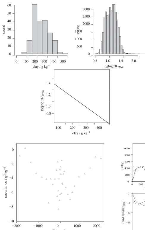
Figure 3(a,b) shows the distributions of the measurements of clay contents and of loglogCR2206 , respectively. A large variability in clay contents was observed over the study area (Figure 3a), as previously shown (Lagacherie et al., 2008). Although the two distributions (Figure 3a,b) appeared as global bell-shapes, they were too dis-symmetric to be strictly considered as normally distributed. Figure 3(c) shows that clay contents measurements were linearly correlated with loglog(CR2206 ) with a coefficient of determination that is slightly less than in Lagacherie et al. (2008) (R2 = 0.55 and 0.58, respectively) because of the addition of new sites.
To verify that the cross-variogram is an appropriate tool for describing the co-variation of clay contents and loglogCR2206 over the study area, it was first necessary to examine the pair of the cross-covariance function (Wackernagel, 1995, p. 133).
positive, which means that the linear model of co-regionalization is strictly conditionally negative definite (in the variogram).
Figure 5 shows that the models fit well to the data. The large range structure (spherical 2000 m) of the loglogCR2206 semi- variogram has a greater relative importance than that of the clay content semi-variogram, which prevents the application of an intrinsic co-regionalization model.
Punctual co-kriging
A punctual co-kriging with cross-validation was performed over the region. Because co-kriging from the whole set of sites with hyperspectral data would require too much computing time, subsets of sites were locally selected to represent optimally the spatial structure of the hyperspectral measurements in the neighbourhood of the prediction location. The co-kriging procedure took into account only (i) all of the sites located less than 400 m from the prediction location and (ii) a sample of the sites located between 400 and 1500 m made by sampling each neighbouring bare-soil field at 15% of the sites, which were randomly selected. All of these parameters were fixed after a
c o u n t c o v a rian c e / g 2 kg − 2 log log C R2206 c o u n t γ (c la y ) γ( c la y L o g lo g CR 2 2 0 6 ) γ( L o g lo g CR 2 2 0 6 ) 60 3000 50 2500 40 2000 30 1500 20 1000 10 500 0 0 100 200 300 400 500 0 0.5 1.0 1.5 2.0 clay / g kg−1 loglogCR2206 1.4 1.2 1.0 0.8 0 −2 100 200 300 400 clay / g kg−1 10000 8000 6000 4000
Figure 3 Data distributions and linear rela-
tionship: (a) distribution of clay content mea- surements, (b) distribution of LogLog CR2206 ,
(c) linear relationship between clay content and
LogLog CR2206. −4 −6 −8 −10 −2000 −1000 0 1000 2000 distance/m
Figure 4 Cross-covariance function (grey triangles) and variogram (black
dots) for clay content (Z1 ).
2000 0 0 −5 −10 −15 −20 0 500 1000 1500 2000 distance/m 0 500 1000 1500 2000 distance/m 0.05 0.04 0.03 0.02 0.01 0.00 0 500 1000 1500 2000 distance/m
trial-and-error procedure, which sought an acceptable compromise between the quality of interpolation and computing cost.
A leave-one-out cross-validation was performed over the set of 200 sites with clay content measurements to obtain a set of observed estimation errors that were compared with the errors
Figure 5 The linear model of co-regionalization for the pair ‘clay content’
and ‘loglogCR2206 ’.
estimated by the co-kriging procedure. The result was that the error variance calculated globally over the 200 sites (2473 g2 kg−2 , and RMSE = 50 g kg – 1 ) was close to that deduced from the cross-validation outputs (2606 g2 kg−2 , and RMSE = 51 g kg – 1 )
propo rt ion in t h is int e rv al 0. 6 0. 7 0. 8 0. 9 0.5 0.6 0.7 0.8 0.9 1.0 p Probability Interval
Figure 6 Plots of the true clay content values falling within probability
from which the interpolations are performed. Again, the error variance estimated by the block co-kriging procedure was used as an estimator of the true error. Four situations were distinguished in the study area: predicted blocks (i) close to clay content measurements and hyperspectral data (≤200 m); (ii) close to clay content measurements and far from hyperspectral data (>200 m); (iii) far from clay content measurements and close to hyperspectral data; and (iv) far from clay content measurements and from hyperspectral data. This classification allowed us to take into account the spatial variation of error related to the local data configurations.
Table 1 shows the performances of the block co-kriging for these four situations with a 100-m block size. As expected, there was a significant decrease of performance with the distance to the data source. These results also showed the usefulness of the hyperspectral data, which improved the predictions where the sites with clay content measurements were close (RMSE = 43 g kg – 1
– 1
intervals estimated by co-kriging (accuracy plot). compared with RMSE = 49 g kg ) and limited the degradation of
with, however, a slight under-estimation of the errors. It must be noted that the error variance of co-kriging was substantially
the performances where the blocks were located far from any sites with clay content measurements (RMSE = 53 g kg – 1 compared with RMSE = 58 g kg – 1 ). Finally, the global error of the 100-m block predictions estimated over the whole area remained fairly smaller than that of ordinary kriging (3567 g2 kg−2 , RMSE =
60 g kg – 1 ), which revealed the added-value of the hyperspectral large (RMSE = error came
49 g kg – 1 ). However, a significant part of this blocks located more than 200 m from any data data.
To evaluate more precisely if the model could predict the local uncertainty, we built an accuracy plot (Figure 6) following the procedure described above. A perfect modelling of local uncertainty would mean that, over the study area, p% of the p-prediction intervals given by the model would include the true value of clay content, which is represented by the 1:1 line in Figure 5. We were fairly close to this situation (Figure 6), but there was an under-estimation of the local uncertainty, mostly for p-prediction intervals ranging from 0.75 to 0.85. Finally, it can be concluded that the co-regionalization model shown in Figure 5 and Equation (10) provided an accurate estimate of the prediction errors for punctual predictions and, consequently, for the block predictions of block means. The latter will be considered in the following section.
Block co-kriging
Block co-kriging was applied over the study area with the same rules as described to define the spatial neighbourhood of data
from
(RMSE = 58 g kg – 1 ), which corresponded to urban or forest areas where it was not possible to sample or find any cultivated (bare) fields with hyperspectral data. Removing these areas significantly decreased the global error (RMSE = 46 g kg – 1 ). In the following, only the first three situations will be considered, as they are together more representative of the situations targeted in this study.
The performances of the predictions for different block sizes are presented in Table 2 for the whole area without considering the 19% urban or forest areas. The estimation error (RMSE) globally decreased as the spatial resolution of predictions (the block size) increased. However, this decrease was moderate between the 50- and 100-m resolution, even resulting in a decrease of the ratio of the explained variance measured by R2 . These results can be explained by the still large spatial autocorrelations for the lag <250 m exhibited by the co-regionalization model (Figure 5), which strongly limited the decrease of variance error that should have been observed if the sites were independent. Finally, for spatial resolutions less than 100 m, at which the block size effect did not play a significant role in decreasing error, it was possible
Table 1 Estimated error variances (RMSE ) of 100-m block prediction of clay contents for different data situations
Closea clay Close clay Far clay sites and far
sites and close sites and farb Far clay sites and CR
2206 sites (urbanized All types except
Type of block CR2206 sites CR2206 sites close CR2206 sites areas and forest) All types urban and forest
Number of blocks 1181 212 483 434 2310 1876 Error variance / g2 kg−2 (RMSE / g kg−1 ) 1835 (43) 2364 (49) 2781 (53) 3339 (58) 2364 (49) 2138 (46)
a Close = <200 m. b Far = >200 m.
Table 2 Estimated performances of the block co-kriging procedure for
different spatial resolutions (urban and forest areas excluded)
Block size 50 100 250 500
data and the quality of the relation between the clay content and the hyperspectral covariable (Lagacherie et al., 2008) were not sufficient to successfully map this effect. Finally, the error maps showed that the error decrease observed in Table 2 was
Numbers of blocks 9707 1876 372 90 associated with a strong decrease of the error variability, especially
Dispersion variance / 4835 4263 2868 1828 for resolutions 250 and 500 m. At these resolutions, the blocks
g2 kg−2
Error variance / g2
kg−2 RMSE / g kg−1
2446 (49) 2138 (46) 1083 (33) 473 (22)
became large enough to include systematically clay content data and bare-soil fields, which strongly diminished and homogenized the prediction error.
R2 0.54 0.49 0.62 0.74
to map half of the total variability of the clay content. For coarser resolutions, the prediction errors were small, and the variability mapped by the block co-kriging procedure was large.
Figure 7 shows images of clay content obtained for different resolutions (first row) and the corresponding error maps. All of the images showed a global increase of clay content from the north to the south of the area. This is probably the effect of the parent material, the Pliocene fluvial deposits, being more clayey than the Miocene marine sediments and its derived colluvions and alluvions. At the finest spatial resolutions (50 and 100 m), it was possible to see more detailed spatial patterns that could represent a relief effect. However, as shown by the error estimations for these resolutions (Table 2), the density of
Discussion
This study aimed to investigate how hyperspectral imagery data available for a set of fields scattered within a study region could help in mapping soil properties over a region at spatial resolutions compatible with those of normal DSM applications. We also con- sidered a set of sites that had laboratory measurements of the soil properties available. We provide an example of the mapping of clay content over a very heterogeneous area located in the south of France.
Block co-kriging was a suitable procedure for both interpolating and spatially aggregating the available input data to produce medium and coarse resolution maps (from 50 to 500 m) of clay content. Although some early applications of co-krigring to the
Figure 7 Images of clay content obtained for
different resolutions (first row) and images of error variance (second row).
mapping of soil properties can be found in the literature (Stein & Corsten, 1991; Odeh et al., 1995), co-kriging has not been used widely in further DSM studies. This may change in the future with the increasing use in DSM of soil sensing covariates such as CR2206 that will be well correlated with a soil property but not exhaustively available in the study area. It must be noted that this procedure can only be applied if an intrinsic or a linear co-regionalization model can be fitted to satisfy the condition of definite positive variogram matrix.
Block predictions of soil properties are not easy to validate because this requires a denser spatial sampling than is required for validating the point predictions. To overcome this problem partially, we proposed first to verify by cross-validation that the co-regionalization model provided a good estimator of the prediction error at punctual sites and then to consider whether the block prediction errors computed from the same co- regionalization model can approximate the unavailable observed error satisfactorily. As well as reducing the validation costs, the great advantage of such a procedure is to provide several images of the same spatial variability (Figure 7) that represent different compromises between accuracy and spatial resolution matching different users’ requirements. However, this validation procedure does not match the usual recommendations for validating DSM results (Lagacherie, 2008). It should therefore be completed by validations from independent samples (Brus et al., 2011). This would require an affordable spatial sampling design that would provide accurate local estimations of block prediction errors and represent the study area well, which would require, respectively, a minimum number of sites within a block and a sufficient amount of validation blocks. Recent advances in soil property measurement technologies (Adamchuk & Viscarra Rossel et al., 2010) should greatly help in fulfilling these requirements.
We found that the hyperspectral image improved the prediction of clay contents substantially in spite of a moderate correlation between clay content and the hyperspectral covariable (R2 = 0.58) and a limited coverage of the study area (3.5%). The former will be ameliorated by improving the correlations thanks to the use of multivariate regression techniques (Ben-Dor et al., 2008; Gomez et al., 2008; Stevens et al., 2010). Progress on the latter will concern either a defined choice of the flying period to increase the chances of getting bare soil surfaces or the use of signal processing algorithms such as spectral un-mixing techniques (Chabrillat et al., 2002; Bartholomeus et al., 2011) or ‘blind source separation’ algorithms (Ouerghemmi et al., 2011) that would allow us to extend the hyperspectral estimations of soil properties to partially vegetated soil surfaces.
Conclusions
The key outputs from this study can be summarized as follows. Block co-kriging is a suitable procedure for using as DSM inputs high-resolution and scattered data such as those produced by hyperspectral imagery. The unavailability of suitable spatial sampling for estimating errors on block mean soil properties can
be partially overcome by using the error variance given by a DSM model previously validated at punctual sites. More research is needed on specific spatial sampling for validating block means estimations from independent samples. A DSM model can produce various maps that represent different compromises between prediction accuracy and spatial resolution. Using hyperspectral data significantly increases the accuracy of the mean clay content estimations. This result should, however, be improved by increasing the accuracy of the hyperspectral indicator and extending the surface covered by hyperspectral data.
Acknowledgements
This research was supported by INRA, IRD and the French National Research Agency (ANR) (ANR-08-BLAN-0284-01). We are indebted to Dr Steven M. de Jong, Utrecht University in the Netherlands, and to Dr Andreas Mueller of the German Aerospace Establishment (DLR) in Wessling, Germany, for providing the 2003 HyMap images used in this study. We are also indebted to Yves Blanca, IRD-UMR LISAH Montpellier, for the soil sampling in 2009 over the vineyard plain of Languedoc.
References
Adamchuk, V.I. & Viscarra Rossel, R.A. 2010. Development of on-the-go proximal sensing systems. In: Proximal Soil Sensing, Progress in Soil
Science, Volume 1 (eds R.A. Viscarra Rossel, A.B. McBratney & B.
Minasny), pp. 15 – 28. Springer, Dordrecht, Heidelberg.
Bartholomeus, H., Kooistra, L., Stevens, A., Van Leeuwen, M., Van Wesemael, B., Ben-Dor, E. et al. 2011. Soil organic carbon mapping of partially vegetated agricultural fields with imaging spectroscopy.
International Journal of Applied Earth Observation & Geoinformation, 13, 81 – 88.
Beisl, U. 2001. Correction of bidirectional effects in imaging spectrometer
data. PhD thesis, Remote Sensing Series 37, RSL, University of Zurich,
Zurich.
Ben-Dor, E., Taylor, R.G., Hill, J., Dematteˆ, J.A.M., Whiting, M.L., Chabrillat, S. et al. 2008. Imaging spectrometry for soil applications.
Advances in Agronomy, 97, 321 – 392.
Brus, D.J., Kempen, B. & Heuvelink, G.B.M. 2011. Sampling for valida- tion of digital soil maps. European Journal of Soil Science, 62, 394 – 407. Chabrillat, S., Goetz, A.F.H., Olsen, H.W. & Krosley, L. 2002. Use of hyperspectral images in the identification and mapping of expansive clay soils and the role of spatial resolution. Remote Sensing of Environment,
82, 431 – 445.
Clark, R.N. & Roush, T.L. 1984. Reflectance spectroscopy: quantitative analysis techniques for remote sensing applications. Journal of Geo-
physical Research, 89, 6329 – 6340.
Cressie, N.A.C. 1991. Statistics for Spatial Data. John Wiley & Sons, New
York.
Gertner, G., Wang, G., Andersol, A.B. & Howard, H. 2007. Combining stratification and up-scaling method – block cokriging with remote sensing imagery for sampling and mapping an erosion cover factor.
Ecological Informatics, 2, 373 – 386.
Gomez, C., Lagacherie, P. & Coulouma, G. 2008. Continuum removal versus PLSR method for clay and calcium carbonate content estimation
from laboratory and airborne hyperspectral measurements. Geoderma,
148, 141 – 148.
Goovaerts, P. 1997. Geostatistics for Natural Resources Evaluation,
Applied Geostatistics Series. Oxford University Press, Oxford.
Goovaerts, P. 1999. Geostatistical modeling of uncertainty in soil science.
Geoderma, 103, 3 – 26.
Grunwald, S. 2009. Multi-criteria characterization of recent digital soil mapping and modeling approaches. Geoderma, 152, 195 – 207. ISSS, ISRIC, FAO 1998. World Reference Base for Soil Resources. World
Soil Resources Report 84, FAO, Rome.
Jenny, H. 1941. Factors of Soil Formation, a System of Quantitative
Pedology. McGraw-Hill, New York.
Jolivet, C., Arrouays, D., Boulonne, L., Ratie, C. & Saby, N. 2006. Le re´seau de mesures de la qualite´ des sols de France (RMQS), Etat d’avancement et premiers re´sultats. Etude et Gestion des Sols, 13, 149 – 164.
Lagacherie, P. 2008. Digital soil mapping: a state of the art. In: Digital Soil
Mapping with Limited Soil Data (eds A. Hartemink, A.B. McBratney &
L. Mendonc¸a-Santos), pp. 3 – 14. Springer, Dordrecht, Heidelberg. Lagacherie, P., Baret, F., Feret, J.B., Madeira Netto, J.S. & Robbez-
Masson, J.M. 2008. Clay and calcium carbonate contents estimated from continuum removal indices derived from laboratory, field and airborne hyper-spectral measurements. Remote Sensing of Environment,
112, 825 – 835.
Leenhardt, D., Voltz, M., Bornand, M. & Webster, R. 1994. Evaluating soil maps for prediction of soil water properties. European Journal of
Soil Science, 45, 293 – 301.
Matheron, G. 1971. The Theory of Regionalised Variables and its
Applications. Ecole des Mines, Fontainebleau.
McBratney, A.B., Mendonc¸a Santos, M.L. & Minasny, B. 2003. On digital soil mapping. Geoderma, 117, 3 – 52.
Odeh, I.O.A., McBratney, A.B. & Chittleborough, D.J. 1995. Further results on prediction of soil properties from terrain attributes: heterotopic cokriging and regression-kriging. Geoderma, 67, 215 – 226.
Ouerghemmi, W., Gomez, C., Nacer, S. & Lagacherie, P. 2011. Applying blind source separation on hyperspectral data for clay content estimation over partially vegetated surface. Geoderma, 163, 227 – 237.
Richter, R. 1996. Atmospheric correction of DAIS hyperspectral image data. Computers & Geosciences, 22, 785 – 793.
Richter, R. & Schla¨pfer, D.A. 2000. A unified approach to parametric geocoding and atmospheric/topographic correction for wide FOV airborne imagery. Part 2: atmospheric correction. In Proceedings 2nd
International EARSeL Workshop on Imaging Spectroscopy , Enschede,
11 – 13 July 2000.
Sanchez, P., Ahamed, S., Carre´, F., Hartemink, A., Hempel, J., Huising, J. et al. 2009. Digital soil map of the world. Science, 325, 680 – 681. Schwanghart, W. & Jarmer, T. 2011. Linking spatial patterns of soil
organic carbon to topography – a case study from south-eastern Spain.
Geomorphology, 126, 252 – 263.
Selige, T., Bohner, J. & Schmidhalter, U. 2006. High resolution topsoil mapping using hyperspectral image and field data in multivariate regression modeling procedures. Geoderma, 136, 235 – 244.
Stein, A. & Corsten, L.C.A. 1991. Universal kriging and cokriging as a regression procedure. Biometrics, 47, 575 – 587.
Stevens, A., Udelhoven, T., Denis, A., Tychon, B., Lioy, R., Hoffmann, L.
et al. 2010. Measuring soil organic carbon in croplands at regional scale
using airborne imaging spectroscopy. Geoderma, 158, 32 – 45. Viscarra Rossel, R.A., Walvoort, D.J.J., McBratney, A.B., Janik, L.J. &
Skjemstad, J.O. 2006. Visible, near-infrared, mid-infrared or combined diffuse reflectance spectroscopy for simultaneous assessment of various soil properties. Geoderma, 131, 59 – 75.
Viscarra Rossel, R.A., McBratney, A.B. & Minasny, B. 2010. Proximal
Soil Sensing, Progress in Soil Science, Volume 1. Springer, Dordrecht,
Heidelberg.
Wackernagel, H. 1995. Multivariate Geostatistics. Springer-Verlag, London.