Leptonic decays of the $D_s$ meson

arXiv:hep-ex/0201024v1 15 Jan 2002

EUROPEAN ORGANIZATION FOR NUCLEAR RESEARCH

CERN–EP/2002–001 8 January 2002

Leptonic decays of the D

s

meson

The ALEPH Collaboration

Abstract

The purely leptonic decays Ds → τν and Ds → µν are studied in a sample

of four million hadronic Z decays collected with the ALEPH detector at the LEP e+_e− _{collider from 1991 to 1995. The branching fractions are extracted}

from a combination of two analyses, one optimized to select Ds → τν decays

with τ → eν ¯ν or µν ¯ν, and the other optimized for Ds → µν decays. The

results are used to evaluate the Dsdecay constant, within the Standard Model:

fDs = [285 ± 19(stat) ± 40(syst)] MeV.

Submitted to Physics Letters B

The ALEPH Collaboration

A. Heister, S. Schael

Physikalisches Institut das RWTH-Aachen, D-52056 Aachen, Germany

R. Barate, I. De Bonis, D. Decamp, C. Goy, J.-P. Lees, E. Merle, M.-N. Minard, B. Pietrzyk

Laboratoire de Physique des Particules (LAPP), IN2_P3_{-CNRS, F-74019 Annecy-le-Vieux Cedex,}

France

G. Boix, S. Bravo, M.P. Casado, M. Chmeissani, J.M. Crespo, E. Fernandez, M. Fernandez-Bosman, Ll. Garrido,15_{E. Graug´es, M. Martinez, G. Merino, R. Miquel,}27_{Ll.M. Mir,}27_{A. Pacheco, H. Ruiz}

Institut de F´isica d’Altes Energies, Universitat Aut`onoma de Barcelona, E-08193 Bellaterra (Barcelona), Spain7

A. Colaleo, D. Creanza, M. de Palma, G. Iaselli, G. Maggi, M. Maggi, S. Nuzzo, A. Ranieri, G. Raso,23

F. Ruggieri, G. Selvaggi, L. Silvestris, P. Tempesta, A. Tricomi,3 _{G. Zito}

Dipartimento di Fisica, INFN Sezione di Bari, I-70126 Bari, Italy

X. Huang, J. Lin, Q. Ouyang, T. Wang, Y. Xie, R. Xu, S. Xue, J. Zhang, L. Zhang, W. Zhao Institute of High Energy Physics, Academia Sinica, Beijing, The People’s Republic of China8

D. Abbaneo, P. Azzurri, O. Buchm¨uller,25 _{M. Cattaneo, F. Cerutti, B. Clerbaux, H. Drevermann,}

R.W. Forty, M. Frank, F. Gianotti, T.C. Greening,29_{J.B. Hansen, J. Harvey, D.E. Hutchcroft, P. Janot,}

B. Jost, M. Kado,27 _{P. Mato, A. Moutoussi, F. Ranjard, L. Rolandi, D. Schlatter, O. Schneider,}2

G. Sguazzoni, W. Tejessy, F. Teubert, A. Valassi, I. Videau, J. Ward

European Laboratory for Particle Physics (CERN), CH-1211 Geneva 23, Switzerland

F. Badaud, A. Falvard,22_{P. Gay, P. Henrard, J. Jousset, B. Michel, S. Monteil, J-C. Montret, D. Pallin,}

P. Perret

Laboratoire de Physique Corpusculaire, Universit´e Blaise Pascal, IN2_P3_{-CNRS, Clermont-Ferrand,}

F-63177 Aubi`ere, France

J.D. Hansen, J.R. Hansen, P.H. Hansen, B.S. Nilsson, A. W¨a¨an¨anen Niels Bohr Institute, DK-2100 Copenhagen, Denmark9

A. Kyriakis, C. Markou, E. Simopoulou, A. Vayaki, K. Zachariadou Nuclear Research Center Demokritos (NRCD), GR-15310 Attiki, Greece

A. Blondel,12 _{G. Bonneaud, J.-C. Brient, A. Roug´e, M. Rumpf, M. Swynghedauw, M. Verderi,}

H. Videau

Laboratoire de Physique Nucl´eaire et des Hautes Energies, Ecole Polytechnique, IN2_P3_-CNRS,

F-91128 Palaiseau Cedex, France V. Ciulli, E. Focardi, G. Parrini

Dipartimento di Fisica, Universit`a di Firenze, INFN Sezione di Firenze, I-50125 Firenze, Italy

A. Antonelli, M. Antonelli, G. Bencivenni, G. Bologna,4_{F. Bossi, P. Campana, G. Capon, V. Chiarella,}

P. Laurelli, G. Mannocchi,5 _{F. Murtas, G.P. Murtas, L. Passalacqua, M. Pepe-Altarelli,}24 _{P. Spagnolo}

Laboratori Nazionali dell’INFN (LNF-INFN), I-00044 Frascati, Italy A. Halley, J.G. Lynch, P. Negus, V. O’Shea, C. Raine,4 _{A.S. Thompson}

Department of Physics and Astronomy, University of Glasgow, Glasgow G12 8QQ,United Kingdom10

S. Wasserbaech

R. Cavanaugh, S. Dhamotharan, C. Geweniger, P. Hanke, G. Hansper, V. Hepp, E.E. Kluge, A. Putzer, J. Sommer, H. Stenzel, K. Tittel, S. Werner,19 _{M. Wunsch}19

Kirchhoff-Institut f¨ur Physik, Universit¨at Heidelberg, D-69120 Heidelberg, Germany16

R. Beuselinck, D.M. Binnie, W. Cameron, P.J. Dornan, M. Girone,1 _{N. Marinelli, J.K. Sedgbeer,}

J.C. Thompson14

Department of Physics, Imperial College, London SW7 2BZ, United Kingdom10

V.M. Ghete, P. Girtler, E. Kneringer, D. Kuhn, G. Rudolph

Institut f¨ur Experimentalphysik, Universit¨at Innsbruck, A-6020 Innsbruck, Austria18

E. Bouhova-Thacker, C.K. Bowdery, A.J. Finch, F. Foster, G. Hughes, R.W.L. Jones, M.R. Pearson, N.A. Robertson

Department of Physics, University of Lancaster, Lancaster LA1 4YB, United Kingdom10

K. Jakobs, K. Kleinknecht, G. Quast,6 _{B. Renk, H.-G. Sander, H. Wachsmuth, C. Zeitnitz}

Institut f¨ur Physik, Universit¨at Mainz, D-55099 Mainz, Germany16

A. Bonissent, J. Carr, P. Coyle, O. Leroy, P. Payre, D. Rousseau, M. Talby

Centre de Physique des Particules, Universit´e de la M´editerran´ee, IN2_P3_{-CNRS, F-13288 Marseille,}

France F. Ragusa

Dipartimento di Fisica, Universit`a di Milano e INFN Sezione di Milano, I-20133 Milano, Italy A. David, H. Dietl, G. Ganis,26

K. H¨uttmann, G. L¨utjens, C. Mannert, W. M¨anner, H.-G. Moser, R. Settles, W. Wiedenmann, G. Wolf

Max-Planck-Institut f¨ur Physik, Werner-Heisenberg-Institut, D-80805 M¨unchen, Germany16

J. Boucrot, O. Callot, M. Davier, L. Duflot, J.-F. Grivaz, Ph. Heusse, A. Jacholkowska, J. Lefran¸cois, J.-J. Veillet, C. Yuan

Laboratoire de l’Acc´el´erateur Lin´eaire, Universit´e de Paris-Sud, IN2_P3_{-CNRS, F-91898 Orsay Cedex,}

France

G. Bagliesi, T. Boccali, L. Fo`a, A. Giammanco, A. Giassi, F. Ligabue, A. Messineo, F. Palla, G. Sanguinetti, A. Sciab`a, R. Tenchini,1

A. Venturi,1

P.G. Verdini

Dipartimento di Fisica dell’Universit`a, INFN Sezione di Pisa, e Scuola Normale Superiore, I-56010 Pisa, Italy

G.A. Blair, G. Cowan, M.G. Green, T. Medcalf, A. Misiejuk, J.A. Strong, P. Teixeira-Dias, J.H. von Wimmersperg-Toeller

Department of Physics, Royal Holloway & Bedford New College, University of London, Egham, Surrey TW20 OEX, United Kingdom10

R.W. Clifft, T.R. Edgecock, P.R. Norton, I.R. Tomalin

Particle Physics Dept., Rutherford Appleton Laboratory, Chilton, Didcot, Oxon OX11 OQX, United Kingdom10

B. Bloch-Devaux, P. Colas, S. Emery, W. Kozanecki, E. Lan¸con, M.-C. Lemaire, E. Locci, P. Perez, J. Rander, J.-F. Renardy, A. Roussarie, J.-P. Schuller, J. Schwindling, A. Trabelsi,21_{B. Vallage}

CEA, DAPNIA/Service de Physique des Particules, CE-Saclay, F-91191 Gif-sur-Yvette Cedex, France17

N. Konstantinidis, A.M. Litke, G. Taylor

Institute for Particle Physics, University of California at Santa Cruz, Santa Cruz, CA 95064, USA13

C.N. Booth, S. Cartwright, F. Combley,4_{M. Lehto, L.F. Thompson}

K. Affholderbach,28_{A. B¨ohrer, S. Brandt, C. Grupen, A. Ngac, G. Prange, U. Sieler}

Fachbereich Physik, Universit¨at Siegen, D-57068 Siegen, Germany16

G. Giannini

Dipartimento di Fisica, Universit`a di Trieste e INFN Sezione di Trieste, I-34127 Trieste, Italy H. He, J. Putz, J. Rothberg

Experimental Elementary Particle Physics, University of Washington, Seattle, WA 98195 U.S.A. S.R. Armstrong, K. Berkelman, K. Cranmer, D.P.S. Ferguson, Y. Gao,20

S. Gonz´alez, O.J. Hayes, H. Hu, S. Jin, J. Kile, P.A. McNamara III, J. Nielsen, Y.B. Pan, J.H. von Wimmersperg-Toeller, W. Wiedenmann, J. Wu, Sau Lan Wu, X. Wu, G. Zobernig

Department of Physics, University of Wisconsin, Madison, WI 53706, USA11

G. Dissertori

Institute for Particle Physics, ETH H¨onggerberg, 8093 Z¨urich, Switzerland.

1_{Also at CERN, 1211 Geneva 23, Switzerland.}

2_{Now at Universit´e de Lausanne, 1015 Lausanne, Switzerland.}

3_{Also at Dipartimento di Fisica di Catania and INFN Sezione di Catania, 95129 Catania, Italy.} 4_Deceased.

5_{Also Istituto di Cosmo-Geofisica del C.N.R., Torino, Italy.}

6_{Now at Institut f¨ur Experimentelle Kernphysik, Universit¨at Karlsruhe, 76128 Karlsruhe, Germany.} 7_{Supported by CICYT, Spain.}

8

Supported by the National Science Foundation of China.

9

Supported by the Danish Natural Science Research Council.

10

Supported by the UK Particle Physics and Astronomy Research Council.

11_{Supported by the US Department of Energy, grant DE-FG0295-ER40896.}

12_{Now at Departement de Physique Corpusculaire, Universit´e de Gen`eve, 1211 Gen`eve 4, Switzerland.} 13_{Supported by the US Department of Energy, grant DE-FG03-92ER40689.}

14_{Also at Rutherford Appleton Laboratory, Chilton, Didcot, UK.} 15_{Permanent address: Universitat de Barcelona, 08208 Barcelona, Spain.}

16_{Supported by the Bundesministerium f¨ur Bildung, Wissenschaft, Forschung und Technologie,}

Germany.

17_{Supported by the Direction des Sciences de la Mati`ere, C.E.A.} 18_{Supported by the Austrian Ministry for Science and Transport.} 19_{Now at SAP AG, 69185 Walldorf, Germany.}

20_{Also at Department of Physics, Tsinghua University, Beijing, The People’s Republic of China.} 21_{Now at D´epartement de Physique, Facult´e des Sciences de Tunis, 1060 Le Belv´ed`ere, Tunisia.} 22_{Now at Groupe d’Astroparticules de Montpellier, Universit´e de Montpellier II, 34095, Montpellier,}

France

23

Also at Dipartimento di Fisica e Tecnologie Relative, Universit`a di Palermo, Palermo, Italy.

24

Now at CERN, 1211 Geneva 23, Switzerland.

25

Now at SLAC, Stanford, CA 94309, U.S.A.

26_{Now at INFN Sezione di Roma II, Dipartimento di Fisica, Universit´a di Roma Tor Vergata, 00133}

1

Introduction

The leptonic decays of the Ds meson are interesting because they open a window onto

the strong interactions of the constituent quarks of the Ds. The absence of strong

interactions among the final state particles makes the interpretation of the measurements particularly straightforward. The information gained is useful in understanding other processes involving heavy pseudoscalar mesons.

The decay Ds→ lν is the second-generation analogue of charged pion decay, π+ → lν.

The Ds → lν decay proceeds via the Cabibbo allowed annihilation of the c and ¯s quarks

in the Ds; the rate depends on the c¯s wavefunction at zero separation.1 The annihilation

amplitude is characterized by the Ds decay constant fDs, defined as

ifDsp

(Ds)

µ = hDs|¯cγµγ5s|0i . (1)

In the Standard Model the leptonic branching fraction is then given by B(Ds → lν) = G2 F 8π τDsf 2 Ds|Vcs| 2_m Dsm 2 l 1 − m2 l m2 Ds !2 , (2)

where τDs is the mean lifetime of the Ds, Vcs is the relevant CKM matrix element, mDs is

the mass of the Ds, and ml is the mass of the lepton.

It is worthwhile to measure fDs because it characterizes the structure of the Ds meson

and can be calculated in various theoretical models. Lattice QCD is now generally considered to be the most reliable method for calculating the pseudoscalar meson decay constants; recent results yield a prediction of fDs = 255 ± 30 MeV [1]. An important

application of the lattice QCD calculations of decay constants is in the evaluation of the third-generation Cabibbo-Kobayashi-Maskawa matrix elements. Constraints on these elements are obtained from measurements of B0_{- ¯B}0 _{mixing and rely on theoretical}

estimates of fB, which is experimentally inaccessible at present. A measurement of fDs

therefore serves as a useful check of the theoretical methods.

The relative branching fractions for Ds → eν, µν, and τν are known precisely in the

Standard Model. From Eq. 2, the ratios of branching fractions are B(Ds→ eν)/B(Ds →

τ ν) = 2.5 × 10−6 _{and B(D}

s → µν)/B(Ds → τν) = 0.103. The helicity suppression in

these decays leads to an extremely small branching fraction for the electron mode. An investigation of the muon and tau modes is presented in this paper.

The helicity suppression is lifted if a photon is radiated from one of the quarks, giving Ds → γlν. The analysis of Ref. [2] leads to an estimate of the ratio r = B(Ds →

γµν)/B(Ds → µν) ∼= 0.014 to 0.11 with B(Ds → γeν) ∼= B(Ds → γµν). The prediction

in [3] is smaller, r ∼= 0.0059. In either case, the effect of Ds → γlν decays on the present

investigation would be small or negligible, and no correction is made for these decays. The data sample and detector are briefly described in Section 2. Two analyses are then presented, one optimized to select Ds → τν decays (Section 3) and one optimized to

select Ds→ µν decays (Section 4). The systematic errors are discussed in Section 5, and

the combined results and conclusions are given in Section 6.

1

2

Data sample and apparatus

The analyses are based on a data sample collected with the ALEPH detector at the LEP e+_e− _{collider in 1991 through 1995, at or near the peak of the Z resonance. The sample}

corresponds to 3.97 × 106 _{produced e}+_e−

→ q¯q events.

Detailed descriptions of the ALEPH detector and its performance may be found in [4, 6]. The tracking system consists of a high-resolution silicon strip vertex detector (VDET), a cylindrical drift chamber (the inner tracking chamber or ITC), and a large time projection chamber (TPC). The VDET comprises two layers of double-sided silicon strip detectors at average radii of 6.3 and 10.8 cm. The spatial resolution for the r-φ and z projections (transverse to and along the beam axis, respectively) is 12 µm at normal incidence. The angular coverage is |cos θ| < 0.85 for the inner layer and |cos θ| < 0.69 for the outer layer. The ITC has eight coaxial wire layers at radii from 16 to 26 cm. The TPC provides up to 21 three-dimensional coordinates per track at radii between 40 and 171 cm, as well as measurements of the specific ionization energy loss (dE/dx) of charged particles. The tracking detectors are contained within a superconducting solenoid, which produces an axial magnetic field of 1.5 T. Charged tracks measured in the VDET-ITC-TPC system are reconstructed with a momentum resolution of ∆p/p = 6 ×10−4_p

t⊕0.005

(pt in GeV/c). An impact parameter resolution of 22 µm in the r-φ plane is achieved for

muons from Z → µ+_µ− _{having at least one VDET r-φ hit. These performance figures}

reflect the improvements obtained from the 1998 reprocessing of the ALEPH LEP1 data set with enhanced event reconstruction algorithms [7].

Surrounding the TPC is an electromagnetic calorimeter (ECAL), a lead/wire-chamber sandwich operated in proportional mode. The calorimeter is read out via projective towers subtending typically 0.9◦

×0.9◦ _{which sum the deposited energy in three sections in depth.}

Beyond the ECAL lies the solenoid, followed by a hadron calorimeter (HCAL), which uses the iron return yoke as absorber and has an average depth of 1.50 m. Hadronic showers are sampled by 23 planes of streamer tubes, providing a digital hit pattern and inducing an analog signal on pads arranged in projective towers. The HCAL is used in combination with two layers of muon chambers outside the magnet for µ identification.

The measurements of charged particle momenta and of energy depositions in the calorimeters, combined with the identification of photons, electrons, and muons, are used to produce a list of charged and neutral energy flow particles in each event [6].

3

D

→

τ ν analysis

The first analysis [8] is designed to search for the decay chain e+_e− _{→ c¯c, c → D}

s→ τν,

with τ → eν ¯ν or τ → µν ¯ν. The electron and muon channels are treated separately. As the final state under study contains three neutrinos, the signature of these decays is an identified lepton and large missing energy in one hemisphere of the event.

Although the e+_e− _{→ b¯b event sample contains more D}

s mesons than the c¯c sample,

the Ds → lν signal is more difficult to isolate in b¯b events due to the softer Ds spectrum

and the large number of semileptonic b decays. Cuts are therefore applied to remove b¯b events, and the analyses are optimized to select Ds decays in c¯c events.

3.1

Event selection

Hadronic Z decays are preselected using charged tracks [9]. Backgrounds from two-photon interactions and dilepton events are reduced to a negligible level by means of additional cuts on the numbers of reconstructed charged and neutral particles. The event thrust axis is required to satisfy |cos θthrust| < 0.8 to select events within the acceptance of the vertex

detector. Each event is then separated into two hemispheres by the plane perpendicular to the thrust axis. The total energy of each hemisphere is calculated and the hemisphere with larger missing energy is selected if it contains an identified lepton (e or µ). Electron identification is based on the shower shape in the electromagnetic calorimeter and the ionization in the time projection chamber; muon identification makes use of the digital pattern information in the hadron calorimeter and hits in the muon chambers [10]. If more than one lepton is present in the selected hemisphere, the one with the highest momentum is considered. The missing energy in the hemisphere is required to be greater than 5 GeV to reduce the background. The hemisphere invariant masses are taken into account in the calculation of the expected hemisphere energies [11].

To further reduce the background from b¯b events, cuts are applied to a set of hemisphere variables based on the pseudorapidities and impact parameters of the charged tracks. The energy flow particles are clustered into jets by means of the JADE algorithm with ycut = 0.003. The pseudorapidity η of a particle is then defined as η = − ln tan(α/2),

where α is the laboratory angle between the particle and the nearest jet axis. The reconstructed particles in c¯c events tend to have larger pseudorapidities than those in b¯b events because of the lower mass of c hadrons compared to b hadrons. An existing ALEPH lifetime-based b tag algorithm [12] was modified to include a dependence on the pseudorapidity of the charged tracks. The tracks in each hemisphere are divided into two groups, one with η ≥ 5.1 and one with η < 5.1. For each group, the confidence level for the hypothesis that all tracks originate from the Z production point is then calculated. The selected lepton track is not included in this calculation. To reject b¯b events, a cut is made on the confidence level for the low-η group in each hemisphere. A further rejection of c¯c background events2 _{is obtained by cutting on the confidence level for the high-η}

group in the hemisphere containing the lepton; with the lepton excluded, signal events have only fragmentation tracks in the lepton hemisphere and can be distinguished from c¯c background events.

The momentum and energy of the Ds candidate are reconstructed from the observed

charged and neutral particles in the event by excluding the lepton l and applying four-momentum conservation: ~ PDs = − X i6=l ~ Pi EDs = √ s −X i6=l Ei .

This procedure is based on the assumption that no neutrinos are produced in the hemisphere opposite the Ds candidate. A kinematic fit is performed in which the energies

of all reconstructed particles (except the lepton) are varied such that the constraint

2_{Throughout this paper, light quark-antiquark (denoted “uds”), c¯c, and b¯b background events are}

[E2 Ds − P 2 Dsc 2_]1/2 _{= M} Dsc

2 _{= 1.968 GeV is satisfied. The energy resolutions for charged,}

neutral electromagnetic, and neutral hadronic particles are parametrized from simulated events. The kinematic fit improves the energy resolution of Ds candidates from 6.7 GeV

to 3.5 GeV. The background is further reduced by the requirement that the fitted Ds

energy be greater than 22.5 GeV. The selection efficiency for c¯c → Ds → τν events is

2.5% (3.3%) in the electron (muon) channel [including the factor of B(τ → lν ¯ν)]. This procedure selects 3956 and 6637 events in the electron and muon channels, respectively.

3.2

Linear discriminant analysis

A linear discriminant analysis is performed on Monte Carlo events to search for an optimal linear combination of event variables so that maximum discrimination between signal and background is achieved. Two discriminating variables, Uc and Ub, are created to

distinguish the c¯c → Ds → τν signal events from c¯c and b¯b backgrounds, respectively;

the backgrounds arise mainly from semileptonic c and b decays. Nine variables are selected to form Uc and ten for Ub. The variables with the greatest discrimination power include

the fitted Ds momentum, the angle between the lepton and the Ds direction in the Dsrest

frame, several b tag variables, and the lepton transverse momentum with respect to the nearest jet axis. The definitions of Uc and Ub are optimized independently in the electron

and muon channels. The distributions of Ub versus Uc are shown in Figs. 1 and 2.

The branching fraction B(Ds → τν) is extracted from a maximum likelihood fit to the

unbinned Ub versus Uc distribution in each channel. The two-dimensional fitting function

consists of one signal and three background (uds, c¯c, and b¯b) components. Although the analysis is optimized to select Ds → τν decays, some Ds → µν decays are also accepted.

Because these two decay rates are both proportional to f2

Ds, both types of decays are

considered to be part of the signal in the fit to the data. Leptonic D+ _{decays also pass}

the selection and are included in the signal. The production of Ds and D+ mesons in the

remaining b¯b events must be taken into account as well. The signal component of the fitting function is therefore taken to be the combination of Ds and D+ decays to τ ν and

µν in c¯c and b¯b events. The relative normalizations of these eight contributions are fixed according to Eq. 2 and the measured charm production rates [13, 14]; fDs/fD = 1.11

+0.06 −0.05

from lattice QCD calculations [15]; Rc and Rb from the Standard Model fit in [13]; |Vcs|

and |Vcd| from [16]; the Ds and D+ lifetimes from [16]; and particle masses from [16].

The normalizations are shown in Table 1. Leptonic D+ _{decays are Cabibbo suppressed}

and contribute less than 8% of the total signal. Each component of the fitting function is parametrized as the sum of up to five two-dimensional correlated Gaussian functions from a fit to simulated events.

A program based on JETSET 7.4 [17] and tuned to ALEPH data [18] was used to generate the Monte Carlo sample of 15 million e+_e−

→ q¯q background events (including 3.7 million c¯c and 6.6 million b¯b events) and 370 000 events containing Ds and D+

leptonic decays. The polarization of the τ is taken into account in the simulation of (pseudoscalar) → τν decays.

The free parameters in the fit to the data are the numbers of events in the signal and the three background components. The fitting procedure is tested with Monte Carlo events to be free of bias.

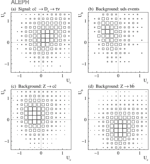
−1 0 1 −1 0 1 U_c U b (a) Signal: cc ¯ → D_s →τν −1 0 1 −1 0 1 U_c U b

(b) Background: uds events

−1 0 1 −1 0 1 U_c U b (c) Background: Z → cc¯ −1 0 1 −1 0 1 U_c U b (d) Background: Z → bb–

Figure 1: Monte Carlo Ub versus Uc distributions in the electron channel of the τ ν

analysis, after all cuts: (a) signal, c¯c → Ds→ τν; (b) uds background; (c) c¯c background;

(d) b¯b background. The area of the square in each bin is proportional to the number of entries. The distributions are shown with arbitrary normalizations.

−1 0 1 −1 0 1 U_c U b (a) Signal: cc ¯ → D_s→τν −1 0 1 −1 0 1 U_c U b

(b) Background: uds events

−1 0 1 −1 0 1 U_c U b (c) Background: Z → cc¯ −1 0 1 −1 0 1 U_c U b (d) Background: Z → bb–

Figure 2: Monte Carlo Ubversus Ucdistributions in the muon channel of the τ ν analysis,

after all cuts: (a) signal, c¯c → Ds → τν; (b) uds background; (c) c¯c background; (d) b¯b

Table 1: Relative normalizations of the contributions to the signal in the Ds→ τν analysis.

Fraction of signal (%)

Source e channel µ channel

c¯c → Ds → τν 76.9 52.4 c¯c → Ds → µν 0.5 26.4 b¯_{b → D}s → τν 17.4 10.7 b¯_{b → D}s → µν 1.2 3.1 c¯c → D+ _{→ τν 3.4 2.3} c¯c → D+ _{→ µν 0.1 4.4} b¯_{b → D}+_{→ τν 0.4 0.4} b¯_{b → D}+_{→ µν 0.2 0.4} Total 100.0 100.0

Table 2: Fitted numbers of signal and background events in data in the Ds → τν analysis.

Only the statistical uncertainties from the fit are shown.

Component e channel µ channel

Signal _{306 ± 62 575 ± 84}

uds background _{111 ± 56 455 ± 139}

c¯c background _{2310 ± 101 3750 ± 182}

b¯b background _{1228 ± 56 1857 ± 74}

3.3

Results

The projections of the two-dimensional fits to the data are shown in Figs. 3 and 4. The fitted numbers of signal and background events are listed in Table 2. The fitted branching fractions from the electron and muon channels are B(Ds → τν) = [5.86 ± 1.18(stat)]%

and [5.78 ± 0.85(stat)]%, respectively.

The goodness of fit is evaluated by comparing the likelihood value obtained from each fit to the data with the distribution of likelihoods obtained from fits to many toy Monte Carlo samples. The fitting functions are used to define the parent distributions in generating these samples. The fit confidence levels are calculated to be 83% in the electron channel and 81% in the muon channel; the Ub versus Uc distributions in the

data are well described by the fitting functions. The same projections are also shown in Figs. 3 and 4 after subtraction of the fitted background components. The distribution of the excess events is consistent in shape with the Monte Carlo prediction for the signal.

It is desirable to visualize the results of the two-dimensional fits in one-dimensional distributions. For this purpose, the purity P of each event is calculated. The purity of event i is defined as Pi = S(U(i) c , U (i) b )

S(U(i)c , U(i)_b ) + B(U(i)c , U(i)_b )

, where U(i)

c and U (i)

b are the values of the discriminant variables for event i, and S and

0 200 400 600 800 −2 −1 0 1 2

Electron Channel

(a)

(b)

(c)

(d)

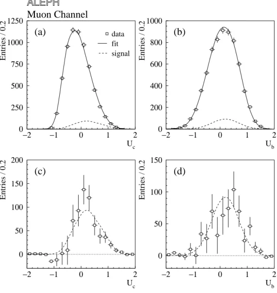
Figure 3: Projections of the fit to the data in the electron channel of the Ds → τν

analysis: (a) Uc distribution; (b) Ub distribution. The data are shown by the squares

with error bars. The solid curves are the fitted distributions, while the dashed curves show the signal contributions. The same distributions are shown in (c) and (d), after subtraction of the fitted backgrounds.

0 250 500 750 1000 1250 −2 −1 0 1 2

Muon Channel

(a)

(b)

(c)

(d)

Figure 4: Projections of the fit to the data in the muon channel of the Ds→ τν analysis:

(a) Uc distribution; (b) Ub distribution. The data are shown by the squares with error

bars. The solid curves are the fitted distributions, while the dashed curves show the signal contributions. The same distributions are shown in (c) and (d), after subtraction of the fitted backgrounds.

results of the fit. The distributions of P are quite different for signal and background events. The purity distributions from the electron and muon channels are shown in Figs. 5a and b; the background-subtracted distributions are given in Figs. 5c and d. These figures show that the shapes of the observed purity distributions agree with the expectations. In particular, the shape of the data distribution in each channel after background subtraction is consistent with the simulated signal and inconsistent with the simulated background.

4

D

→

µν analysis

The second analysis [19] is optimized to select e+_e−

→ c¯c events containing the decay Ds → µν.

4.1

Event selection

The same preselection of hadronic Z decays is performed as in the τ ν analysis. A cut on the number of reconstructed charged tracks coming from the area of the interaction point is applied to reduce the background from dilepton events. The event thrust axis is required to satisfy |cos θthrust| < 0.8. A loose muon identification algorithm [19], requiring

either muon chamber hits or a muon-like digital pattern in the HCAL, is used to select muon candidates. If more than one muon is present in the event, the one with highest momentum is selected.

A kinematic fit is then performed in order to improve the resolution on the missing momentum, assumed to arise from the undetected neutrino from Ds → µν. In this fit,

the missing mass is constrained to be zero and the Ds displacement direction (from the

event primary vertex to the Ds decay vertex, i.e., an unknown point on the muon track) is

constrained to be parallel to the Dsmomentum direction. This constraint is equivalent to

requiring that the reconstructed neutrino direction be parallel to a plane containing the primary vertex and the muon track. The energies of the reconstructed charged and neutral particles are varied in the fit, while their directions are held constant. The muon track impact parameters and the coordinates of the event primary vertex are also allowed to vary within their uncertainties. The kinematic fit improves the resolution on the neutrino energy from 5.7 GeV to 2.8 GeV and on the neutrino direction from 8.9◦ _{to 6.2}◦_.

The b¯b background and some of the c¯c background are further reduced by cuts on the track pseudorapidities and impact parameters, as described in Section 3.1. Finally, a hard cut is made on the fitted energy of the Ds candidate, Eµ+ Eν > 28 GeV. This

procedure selects 7164 events in the data.

4.2

Linear discriminant analysis

Linear discriminant variables Ucand Ubare optimized to distinguish c¯c → Ds→ µν signal

events from c¯c and b¯b backgrounds, respectively. Each of the linear discriminant variables is a combination of seven event variables. The variables with the greatest discrimination power include the muon momentum, the fitted neutrino momentum, and several b- and c-tag neural network outputs. The Ub versus Uc distributions for signal and background

1 10 102 103 0 0.2 0.4 0.6 Purity Entries / 0.088 1 10 102 103 0 0.2 0.4 0.6 Purity Entries / 0.088 1 10 102 103 0 0.2 0.4 0.6 Purity Entries / 0.088 1 10 102 103 0 0.2 0.4 0.6 Purity Entries / 0.088

Electron Channel Muon Channel

(a)

(b)

(c)

(d)

Figure 5: Distributions of purity P , in the (a) electron channel and (b) muon channel of the Ds → τν analysis. The data are shown by the squares with error bars. The

histograms show the Monte Carlo distributions for the background (dotted) and for the signal plus background (solid). The Monte Carlo histograms are normalized according to the results of the fits to the data. The plots in (c) and (d) show the same distributions after subtraction of the fitted backgrounds; the squares are the data and the histograms are the Monte Carlo signal distributions. The error bars in all four plots reflect the statistical errors in the data.

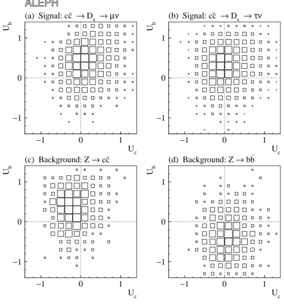
−1 0 1 −1 0 1 U_c Ub (a) Signal: cc ¯ → D_s →µν −1 0 1 −1 0 1 U_c Ub (b) Signal: cc ¯ → D_s →τν −1 0 1 −1 0 1 U_c Ub (c) Background: Z → cc¯ −1 0 1 −1 0 1 U_c Ub (d) Background: Z → bb–

Figure 6: Monte Carlo Ub versus Uc distributions in the Ds → µν analysis, after all

cuts: (a) signal, c¯c → Ds → µν; (b) c¯c → Ds → τν, which is also included in the

signal component of the fitting function; (c) c¯c background; (d) b¯b background. The distributions are shown with arbitrary normalizations.

Table 3: Relative normalizations of the contributions to the signal in the Ds→ µν analysis. Source Fraction (%) c¯c → Ds → τν 49.6 c¯c → Ds → µν 26.7 b¯_{b → D}s → τν 12.6 b¯_{b → D}s → µν 3.5 c¯c → D+_{→ τν 2.2} c¯c → D+_{→ µν 4.3} b¯_{b → D}+_{→ τν 0.6} b¯_{b → D}+_{→ µν 0.5} Total 100.0

4.3

Results

The numbers of signal and background events are extracted from the data by means of a maximum likelihood fit to the (Uc, Ub, Mµν) distribution, where Mµν is the invariant mass

of the Dscandidate after the kinematic fit. The three-dimensional region −0.6 < Uc < 1.0,

−0.8 < Ub< 1.4, and Mµν < 5 GeV/c2 is divided into 6×6×11 bins in the fit. The fitting

functions are constructed from simulated events and a procedure is applied to smooth the distributions to reduce the bias that results from limited Monte Carlo statistics near the edges of the space.

As in the Ds → τν analysis, the signal component consists of eight contributions from

Ds and D+ decays to τ ν and µν in c¯c and b¯b events; the relative normalizations of these

contributions are again fixed according to the Standard Model expectations (Table 3). Although the µν invariant mass provides some separation between Ds → µν decays and

the backgrounds, the Ds → µν decay mode comprises only 30% of the signal and cannot

be clearly isolated in a fit to the (Uc, Ub, Mµν) distribution. With the Standard Model

constraint B(Ds → µν)/B(Ds→ τν) = 0.103 imposed in the fit, this analysis nevertheless

yields additional information on fDs. (Fits in which this constraint is not imposed are

described in Section 5.3.)

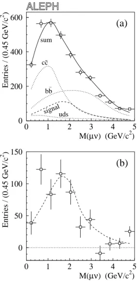
The fitted numbers of events are 553±93 signal events, 166±47 uds background events, 1251 ± 71 c¯c background events, and 1291 ± 62 b¯b background events. Figure 7 shows the fit projection on the Mµν axis. After correction for a bias of +8.2% in the smoothing

and fitting procedure, the fit result corresponds to B(Ds → µν) = [0.68 ± 0.11(stat)]%.

The goodness of fit is characterized by a confidence level of 69%.

The purity distribution from the Ds → µν analysis is shown in Fig. 8. The purity is

defined as in Section 3.3, except in this case the signal and background distributions S and B are binned functions of Uc, Ub, and Mµν. Again the signal and background events

have distinct distributions, and the shape of the background-subtracted data distribution agrees with that of the simulated signal.

0 200 400 600 0 1 2 3 4 5 M(µν) (GeV/c2) Entries / (0.45 GeV/c 2 ) sum cc¯ bb– signaluds

(a)

(b)

Figure 7: (a) Mµν projection of the fit to the data in the Ds → µν analysis. The data

are shown by the squares with error bars. The solid curve is the fitted distribution. The dashed curve shows the signal contribution, while the dotted curves indicate the three background contributions. The data and fitted signal distributions are shown in (b), after subtraction of the fitted backgrounds.

10 102 103 0 0.2 0.4 0.6 Purity Entries / 0.05 10 102 103 0 0.2 0.4 0.6 Purity Entries / 0.05

(a)

(b)

Figure 8: (a) Distribution of purity P in the Ds → µν analysis. The data are shown

by the squares with error bars. The histograms show the Monte Carlo distributions for the background (dotted) and for the signal plus background (solid). The Monte Carlo histograms are normalized according to the results of the fit to the data. (b) Purity distribution after subtraction of the fitted backgrounds; the squares are the data and the histogram is the Monte Carlo signal distribution. The errors in both plots reflect the statistical errors in the data.

Table 4: Relative systematic uncertainties on B(Ds → lν).

Uncertainty (%)

Source Ds → τν (e) Ds → τν (µ) Ds→ µν

Charm hadron production 27.0 22.8 19.6

c fragmentation 16.7 14.8 12.1

b fragmentation 9.0 5.9 4.1

Lepton spectra in b and c decays 5.5 3.6 3.1

Lepton rates in b¯b events 0.3 0.1 1.7

Detector resolution 13.6 12.7 4.0

Monte Carlo statistics 7.2 6.0 8.8

Bias in fitting procedure — — 4.1

D+ _{→ ¯K}0_µ+_{ν form factor 0.5 0.5 1.5}

fDs/fD 0.2 0.7 1.4

Total 36.8 31.4 26.0

5.1

Evaluation of systematic uncertainties

In both analyses, the shapes of the signal and background fitting functions are taken from simulated events. The physics parameters that can affect these shapes are taken into account in the systematic uncertainties on the branching fractions.

The sources of systematic error are summarized in Table 4. The magnitudes of the systematic errors are estimated by measuring the branching fractions from a Monte Carlo sample, reweighting the Monte Carlo events to simulate a variation in a parameter, then measuring the branching fractions again. In each case the quoted systematic uncertainty is taken to be the quadratic sum of the observed shift and the statistical uncertainty on the shift.

The uncertainties on the production rates of D+_{, D}0_{, D}

s, and charm baryons

from [13, 14] are taken into account, including correlations. The Ds production rates have

large uncertainties due mainly to the large uncertainty on the absolute scale of branching fractions for hadronic Ds decays; these parameters give the largest contributions to the

systematic error on the leptonic branching fractions because they directly govern the number of produced Ds mesons in the data sample.

The Monte Carlo events are weighted to match the mean scaled energies hxE(c)i =

0.484 ± 0.008 and hxE(b)i = 0.702 ± 0.008 of charm and b hadrons given in [20]; the

uncertainties on those fragmentation parameters are propagated to the leptonic branching fractions.

The shapes of the lepton energy spectra in b and c decays are varied according to the prescription given in [21]. The b → l and b → c → ¯l fractions and uncertainties are taken from [13].

The detector resolution on missing energy and momentum is dominated by the errors on neutral particle energies. The energy resolutions for neutral energy flow particles are studied in samples of hadronic Z decays in data and Monte Carlo. The electromagnetic and

fit in which the total energy in each event is constrained to√s and the total momentum is constrained to zero. Although the four-momentum carried away by neutrinos and objects at low angles is not taken into account in this procedure, a useful comparison of the energy resolutions in data and Monte Carlo can nevertheless be made. A discrepancy of less than 4% in the neutral particle energy resolution is observed, and the effect on the branching fractions is estimated by further smearing the neutral energies in the Monte Carlo events that are used to build the fitting functions.

The Monte Carlo statistical uncertainty is estimated by generating many toy Monte Carlo samples, using the fitting functions obtained from the full simulation as the parent distributions. This procedure reveals a +8.2% bias in the smoothing and fitting procedure in the Ds → µν analysis, and a systematic uncertainty equal to half the bias is assigned. As

a cross check, a fit to the data in this channel is also performed with an algorithm in which the statistical fluctuations in the Monte Carlo distributions are taken into account [22]; the fitted number of signal events is within 2% of that obtained with the standard program, after bias corrections.

Other small effects considered are the form factor in D+ _{→ ¯K}0_µ+_{ν decays [23] (an}

important source of background) and the ratio of decay constants fDs/fD from [15].

5.2

Cross check with D

→

φπ decays

A study of Ds → φπ decays is performed as a cross check of the signal efficiencies in the

Ds → lν analyses. Candidate Ds → φπ decays with φ → K+K− are first selected from the

full e+_e−

→ q¯q sample. The dE/dx measurements in the TPC are used to discriminate between pions and kaons. Cuts are also applied on the kaon and pion momenta, the K+_K−

invariant mass, and the decay angle of the φ. The same selection is applied to simulated q¯q events containing Ds → φπ decays.

The KKπ candidates are divided into seven bins of xE = EKKπ/Ebeam, from 0.3 to

1. The number of Ds mesons in each xE bin in the data is evaluated by means of a fit

to the reconstructed KKπ invariant mass distribution for the candidates in that bin. In this fit the signal is described as the sum of two Gaussian functions, and a second pair of Gaussians is included for the D+_{→ φπ contribution; a polynomial function is used for}

the background.

In order to measure the efficiencies of the Ds → lν selections, the pion in each KKπ

combination is treated as the lepton candidate; the kaons are removed from the event and correspond to the missing neutrino(s). After the selection cuts are made, the number of Ds mesons in each xE bin is again extracted from the KKπ invariant mass distribution.

The selection efficiency in each bin is then evaluated in data and Monte Carlo. Some cuts, most notably the lepton identification cuts, cannot be studied with this method. The Ds → τν and Ds→ µν analyses are checked separately.

The following aspects of the Ds → τν analysis are included in the φπ cross check:

the cut on missing energy, the b¯b and dilepton rejection cuts, the kinematic fit, and the cut on the fitted Ds energy. With the kaon candidates excluded from the event, these

operations can be accurately duplicated in the φπ events. The overall efficiency of these cuts as a function of xE, in data and Monte Carlo, is plotted in Fig. 9. The signal

0 0.5 1 0.4 0.6 0.8 1 x_E Efficiency data MC

Figure 9: Efficiency versus xE in data (squares with error bars) and Monte Carlo

(histogram) for the Ds → τν selection cuts listed in the text, as measured from Ds → φπ

decays. The cut on the fitted Ds energy, EDs > 22.5 GeV, corresponds to xE

> ∼0.49. 0 25 50 75 100 1 2 3 4 5

Fitted mass (GeV/c2)

Entries / (0.5 GeV/c

2 )

data MC

Figure 10: Background-corrected distribution of the Ds mass (calculated from the π and

the missing K+_K−_{) after the kinematic fit, in the φπ cross check of the D}

s→ µν analysis.

The data are shown by the squares with error bars, while the histogram shows the Monte Carlo distribution. The number of Ds mesons in each mass bin in the data is obtained

Table 5: Fitted background events relative to the expected numbers in the two channels of the Ds→ τν analysis and in the Ds → µν analysis. The first uncertainty given in each

case is statistical and the second systematic.

Fitted / Expected Background

Background Ds → τν (e) Ds→ τν (µ) Ds → µν

uds _{0.81 ± 0.40 ± 0.58 1.00 ± 0.31 ± 0.42 0.84 ± 0.22 ± 0.17} c¯c _{0.92 ± 0.04 ± 0.06 0.93 ± 0.04 ± 0.07 0.96 ± 0.05 ± 0.08} b¯b _{0.92 ± 0.05 ± 0.05 1.06 ± 0.04 ± 0.05 0.98 ± 0.05 ± 0.06}

the statistical uncertainty of the test (7% relative uncertainty).

A similar φπ cross check is performed for the Ds→ µν analysis. The main differences

with respect to the Ds → τν case are (1) the fitted primary vertex and the impact

parameters of the pion (serving as the muon) are now involved in the kinematic fit, and (2) it is possible to check the resolution on the reconstructed Ds mass. For purposes of

this test, the missing mass is constrained in the kinematic fit to equal the reconstructed K+_K− _{invariant mass on an event-by-event basis. The measured efficiencies in data and}

Monte Carlo are again found to be in agreement. The distributions of reconstructed Ds

mass in data and Monte Carlo are plotted in Fig. 10; the simulated resolution is found to be consistent with that observed in the data.

5.3

Additional checks

Additional checks, described in this section, are performed in order to further investigate the accuracy of the Monte Carlo simulation.

The fitted numbers of uds, c¯c, and b¯b background events are compared with the Monte Carlo predictions in Table 5. The normalization of the predicted numbers is based on the total number of produced e+_e−

→ q¯q events in the data sample. The predictions for Ds → µν are corrected for biases in the fitting procedure. The data and Monte Carlo

are in agreement. A χ2 _{value is computed to characterize this agreement in the D}

s → µν

analysis, taking into account the correlations in the statistical and systematic errors on the normalizations of the three backgrounds. The result is χ2 _{= 0.74 for three degrees of}

freedom (CL = 87%).

The distributions of the event variables used to construct the three sets of linear discriminant variables Uc and Ub are compared in data and Monte Carlo to ensure that

the simulation is reliable. The Monte Carlo plots are normalized according to the results of the fits to the data. No significant discrepancies are found.

Another cross check on the accuracy of the simulation is made by comparing the distributions of certain quantities in data and Monte Carlo in different regions of the (Uc, Ub) space. In each analysis, four disjoint regions in that space are defined with

different relative abundances of the signal and the three backgrounds. The Monte Carlo normalization is again based on the results of the fits to the data. The quantities studied in the Ds → τν analysis include the fitted Ds momentum, the angle between the lepton

the missing energy before the kinematic fit, the µν invariant mass after the kinematic fit, and the fitted proper Ds decay length were considered. The simulation is found to

be consistent with the data in all cases and in all regions of the (Uc, Ub) space. This

check demonstrates that the properties of the backgrounds are correctly reproduced in the Monte Carlo.

The fit to the data in the Ds→ µν analysis was repeated without the Standard Model

constraint on B(Ds → µν)/B(Ds → τν). For this calculation, the signal contributions

from Ds and D+ decays to µν were allowed to vary separately from the τ ν contributions.

The fitted contribution from µν relative to τ ν is found to be somewhat smaller than expected; Monte Carlo experiments show that the unconstrained fit is expected to give a µν/τ ν ratio smaller than the observed value 5% of the time when the events are generated according to the Standard Model ratio. The fitted µν/τ ν ratio is not sensitive to the assumed charm production rates or fragmentation parameters.

Increased sensitivity to B(Ds→ µν) is achieved if the Ds → µν analysis is coupled to

the statistically independent electron channel of the Ds→ τν analysis. The fit described

in the preceding paragraph is repeated with a modified likelihood function in which B(Ds → τν) is constrained according to the value and uncertainty obtained from the

electron channel; after correction for the calculated −1% and +14% biases, respectively, the results are

B(Ds→ µν) = (0.47 ± 0.25)%

B(Ds → τν) = (6.8 ± 1.0)% ,

where the uncertainties are statistical only.

6

Conclusions

Leptonic decays of the Ds meson have been studied in a sample of four million hadronic

Z decays. The Ds → τν analysis gives

B(Ds → τν) = (5.86 ± 1.18 ± 2.16)% , (electron channel)

= _{(5.78 ± 0.85 ± 1.81)% ,} (muon channel) where the measured signal includes some Ds → µν and D+→ lν decays. In the Standard

Model, these branching fractions correspond to the following values of the decay constant fDs:

fDs = (275 ± 28 ± 51) MeV , (electron channel)

= _{(273 ± 20 ± 43) MeV .} (muon channel)

These results are combined, taking into account the common systematic errors [24], to obtain

B(Ds → τν) = (5.79 ± 0.77 ± 1.84)%

The combination has χ2 _{= 0.0024 for 1 degree of freedom (CL = 96%). This measurement}

may be expressed as

f (c → Ds)B(Ds→ τν) = (6.77 ± 0.90 ± 1.49) × 10−3 ,

where f (c → Ds) is the Ds production rate per hemisphere in Z → c¯c events; the relative

uncertainty on this product is smaller than that on B(Ds → τν) due to the reduced

dependence on the assumed Ds production rate.

The analysis optimized for Ds→ µν is also sensitive to Ds → τν decays; a measurement

of the combined signal yields

B(Ds → µν) = (0.68 ± 0.11 ± 0.18)%

when the ratios of the signal components are fixed to their Standard Model values. This measurement corresponds to

fDs = (291 ± 25 ± 38) MeV .

Finally, the three fDs measurements (two from τ ν and one from µν) are combined.

The correlation coefficient k = +0.43 ± 0.34 of the statistical errors in the Ds → µν

analysis and the muon channel of the Ds → τν analysis is evaluated by dividing the data

into ten subsamples. The correlations between the systematic errors are also taken into account. The combined decay constant is

fDs = (285 ± 19 ± 40) MeV

with χ2 _{= 0.51 for 2 degrees of freedom (CL = 78%).}

This result is consistent with recent measurements [16, 25, 26] and with the lattice QCD prediction, fDs = 255 ± 30 MeV [1].

Acknowledgements

We wish to thank our colleagues in the CERN accelerator divisions for the successful operation of LEP. We are indebted to the engineers and technicians in all our institutions for their contribution to the excellent performance of ALEPH. Those of us from nonmember countries thank CERN for its hospitality.

References

[1] C. Bernard, “Heavy Quark Physics on the Lattice”, Nucl. Phys. Proc. Suppl. 94 (2001) 159, hep-lat/0011064.

[2] G. Burdman, T. Goldman, and D. Wyler, “Radiative Leptonic Decays of Heavy Mesons”, Phys. Rev. D51 (1995) 111.

[3] D. Atwood, G. Eilam, and A. Soni, “Pure Leptonic Radiative Decays B±_{, D}

s → lνγ

[4] ALEPH Collaboration, “ALEPH: a Detector for Electron-positron Annihilations at LEP”, Nucl. Instrum. Methods A294 (1990) 121.

[5] B. Mours et al., “The Design, Construction and Performance of the ALEPH Silicon Vertex Detector”, Nucl. Instrum. Methods A379 (1996) 101.

[6] ALEPH Collaboration, “Performance of the ALEPH Detector at LEP”, Nucl. Instrum. Methods A360 (1995) 481.

[7] ALEPH Collaboration, “A Study of the Decay Width Difference in the B0

s- ¯B0s System

Using φφ Correlations”, Phys. Lett. B486 (2000) 286.

[8] L. He, “A Measurement of the Branching Fraction of the Ds Meson Decay into a Tau

and a Neutrino”, Ph.D. thesis, University of Washington, 2000.

[9] ALEPH Collaboration, “Measurement of the Z Resonance Parameters at LEP”, Eur. Phys. J. C14 (2000) 1.

[10] ALEPH Collaboration, “Heavy Quark Tagging with Leptons in the ALEPH Detector”, Nucl. Instrum. Methods A346 (1994) 461.

[11] ALEPH Collaboration, “Measurement of the B0

s Lifetime”, Phys. Lett. B322 (1994)

275.

[12] ALEPH Collaboration, “A Precise Measurement of Γ(Z → b¯b)/Γ(Z → hadrons)”, Phys. Lett. B313 (1993) 535.

[13] The LEP Collaborations, the LEP Electroweak Working Group, and the SLD Heavy Flavor and Electroweak Groups, “A Combination of Preliminary Electroweak Measurements and Constraints on the Standard Model”, preprint CERN-EP/2000-016.

[14] ALEPH Collaboration, “Charm Counting in b Decays”, Phys. Lett. B388 (1996) 648.

[15] T. Draper, “Status of Heavy Quark Physics on the Lattice”, Nucl. Phys. Proc. Suppl. 73 (1999) 43, hep-lat/9810065.

[16] D.E. Groom et al. (Particle Data Group), “Review of Particle Physics”, Eur. Phys. J. C15 (2000) 1.

[17] T. Sj¨ostrand, “High-energy Physics Event Generation with PYTHIA 5.7 and JETSET 7.4”, Comp. Phys. Commun. 82 (1994) 74.

[18] ALEPH Collaboration, “Heavy Flavor Production and Decay with Prompt Leptons in the ALEPH Detector”, Z. Phys. C62 (1994) 179; “Studies of Quantum Chromodynamics with the ALEPH Detector”, Phys. Rep. 294 (1998) 1.

[19] J. Putz, “A Measurement of the Branching Fraction of the Ds Meson to a Muon and

[20] The LEP Heavy Flavour Working Group, “Input Parameters for the LEP/SLD Electroweak Heavy Flavour Results for Summer 1998 Conferences”, LEPHF/98-01 (1998).

[21] The LEP Heavy Flavour Working Group, “A Consistent Treatment of Systematic Errors for LEP Electroweak Heavy Flavour Analyses”, LEPHF 94-001 (1994). [22] HBOOK routine hmcmll; R. Barlow and C. Beeston, “Fitting Using Finite Monte Carlo

Samples”, Comp. Phys. Commun. 77 (1993) 219.

[23] CLEO Collaboration, “Measurement of Exclusive Semileptonic Decays of D Mesons”, Phys. Lett. B317 (1993) 647.

[24] L. Lyons, D. Gibaut, and P. Clifford, “How to Combine Correlated Estimates of a Single Physical Quantity”, Nucl. Instrum. Methods A270 (1988) 110.

[25] BEATRICE Collaboration, “Measurement of the Ds→ µνµ Branching Fraction and

of the Ds Decay Constant”, Phys. Lett. B478 (2000) 31.

[26] OPAL Collaboration, “Measurement of the Branching Ratio for D−

s → τ−ν¯τ Decays”,