Approximating the maximum acyclic subgraph

Approximating the Maximum Acyclic Subgraph

by

Alantha Newman

Submitted to the Department of Electrical Engineering and Computer Science

in partial fulfillment of the requirements for the degree of

Master of Science in Computer Science

at the

MASSACHUSETTS INSTITUTE OF TECHNOLOGY

June 2000

©

Massachusetts Institute of Technology 2000. All rights reserved.

A u th o r ... ...

...

...

...

Department of Electrical Engineering and Computer Science

Spring, 2000

Certified by ...

...

...

..

...

Santosh Vempala

Assistant Professor of Mathematics

Thesis Supervisor

Accepted by ...

Arthur C. Smith

Chairman, Departmental Committee on Graduate Students

MASSACHUSETS INSTITUTE OF TECHNOLOGY

JUN

2 2 2000

Approximating the Maximum Acyclic Subgraph

by

Alantha Newman

Submitted to the Department of Electrical Engineering and Computer Science on May 19, 2000, in partial fulfillment of the

requirements for the degree of Master of Science in Computer Science

Abstract

In this thesis, we study the maximum acyclic subgraph problem: Given a directed graph G = (V, E), find a maximum cardinality subset E' C E such that G = (V, E') is acyclic. The maximum acyclic subgraph problem is an NP-hard optimization problem for which the best-known approximation guarantee is 2. We show that the maximum acyclic subgraph problem cannot be approximated to within 65+ e for any e > 0. The reduction is from Histad's

maximum satisfiability of linear equations modulo 2 with three variables per equation. It is already known that the integrality gap of two basic linear programming relaxations is 2, but we formalize this here since it is not recorded elsewhere. We also study graphs in which the maximum degree is 3 and show that if for any e > 0 there exists a (17/18+E)-approximation

algorithm for the maximum acyclic subgraph problem in such graphs, then there is a 6 > 0

such that there is a (1/2 + 6)-approximation algorithm for the maximum acyclic subgraph problem in general graphs. We give a 8-approximation algorithm for the maximum acyclic

subgraph problem in graphs with maximum degree 3. Thesis Supervisor: Santosh Vempala

Acknowledgments

I thank Santosh Vempala for being my advisor and for patiently teaching me so many new things. I also thank John Dunagan for enthusiastically answering many questions related

Contents

1 Introduction

1.1 The Problem . . . . 1.2 Overview of this Thesis . . . . 2 Inapproximability

2.1 Reduction from 3-SAT . . . . 2.1.1 The Construction . . . . 2.1.2 The Proof . . . . 2.2 Reduction from Linear Equations Modulo 2

2.2.1 The Construction . . . . 2.2.2 The Proof . . . .

3 Linear Programming Relaxations

3.1 Two Integer Programs . . . . 3.2 Linear Program Integrality Gap .

3.3 Constructing Undirected Dense Graphs with High Girth . 4 Restricted Problem

4.1 Eulerian Graphs . . . . 4.2 Degree-3 Graphs . . . . 5 Algorithms for Degree-3 Graphs

5.1 Assumptions . . . . 5.2 Algorithm I . . . . 5.3 Algorithm 2 . . . . 5 . . . . 5 . . . . 5 7 7 7 8 11 11 12 16 16 17 20 22 . . . . 22 . . . . 23 29 29 30 30

. . . .

. . . . . . . . . . . .

Chapter 1

Introduction

Many important and practically motivated optimization problems are NP-hard. Unless P = NP, we cannot efficiently find exact solutions to these problems. One option is to relax the requirement that the size (or cost) of the solution is optimal. Instead, we can look for a solution whose size if provably within some factor of the size of an optimal solution. In this scenario, we want to find an algorithm that yields the best possible factor or approximation ratio. See [11] for an overview of approximation algorithms.

1.1

The Problem

In this paper, we explore the approximability and inapproximability of a particular NP-hard optimization problem known as the maximum acyclic subgraph problem. The maximum acyclic subgraph problem is defined as follows: Given a directed graph G = (V, E), find a

maximum cardinality subset E' C E such that G = (V, E') is acyclic. This problem is an

example of an NP-hard optimization problem for which a simple approximation algorithm offers the best-known guarantee on the size of the solution. For any linear ordering of the vertices, the set of forward edges or the set of backward edges contains at least half the edges. Each set is acyclic. The entire set of edges, E, is an upper bound on the size of an optimal solution. Therefore, the larger of these sets yields a -approximation.

An outstanding open problem is: Can we do better than half of the optimum?

1.2

Overview of this Thesis

In Chapter 2, we show that it is NP-hard to approximate the maximum acyclic subgraph to within 2 + c for any e > 0. This means that if we could find an algorithm with an approximation guarantee of 2 + c for some e > 0, then we could solve the problem exactly. We give a reduction from 3-SAT to the maximum acyclic subgraph problem to illustrate

the idea behind the inapproximability reduction. We then give a reduction from Histad's linear equations modulo 2 with 3 variables per equation, which, although more complicated, yields a better inapproximability constant.

A common tool for finding approximation algorithms for NP-hard optimization problems is linear programming. In Chapter 3, we discuss linear programming relaxations for the maximum acyclic subgraph problem. The basic linear programming relaxation for the maximum acyclic subgraph problem has an integrality gap of 2, i.e. there is a class of graphs for which the true maximum is very close to half the edges, while the linear programming relaxation returns a fractional solution with value very close to the size of the entire edge set. Therefore, we cannot use the basic linear programming relaxation to obtain a better-than-half approximation.

In Chapter 4, we first investigate the maximum acyclic subgraph problem restricted to Eulerian graphs. We present a theorem due to Lovisz and Chen [8] showing that the general problem can be reduced to this restricted problem. We next investigate the maximum acyclic subgraph problem restricted to graphs with maximum degree 3, i.e. in-degree plus out-degree of any vertex in the graph is at most 3. The maximum acyclic subgraph problem remains NP-hard for such graphs [7]. We show that there is a connection between the approximability of degree-3 graphs and general graphs. In particular, we show that if for any c > 0 there exists a (E +E)-approximation algorithm for the maximum acyclic subgraph problem in degree-3 graphs, then there exists a better-than-half approximation algorithm for the maximum acyclic subgraph problem in general graphs.

Finally, in Chapter 5 we show that we can actually approximate the maximum acyclic subgraph in degree-3 graphs to within 8.

Chapter 2

Inapproximability

In this chapter, we will describe two reductions which essentially use the same idea. The first reduction is from 3-SAT and the second reduction is from Histad's linear equations modulo 2 with 3 variables per equation. The idea behind both reductions is that an assignment that satisfies a particular clause corresponds to removing one less edge from the representative clause gadget than an than an assignment that does not satisfy this clause.

2.1

Reduction from 3-SAT

In this section we will give an approximation-preserving reduction from MAX-3-SAT to the maximum acyclic subgraph problem. MAX-3-SAT is defined as the following problem: Given a CNF formula with at most 3 variables per clause, find an assignment of the variables that maximizes the number of satisfied clauses.

2.1.1 The Construction

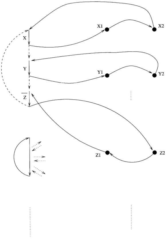
Given a 3-SAT formula F with n variables and m clauses, we construct a corresponding multigraph G using the following rules: (We assume every variable in F appears at least once negated and once unnegated.)

1. For each variable x E F, we create 2 vertices x1 and X2. These two vertices will form

the variable gadget for the variable x.

2. For each clause Ck E F, we create a directed 6-cycle and label each of 3 alternating edges with a distinct literal from the clause Ck. This will be the clause gadget for the clause Ck.

" For an edge (i, j) labeled x in a clause gadget, we add a directed edge from vertex

j to vertex xi, an edge from x, to x2, and an edge from X2 to i.

" _{For an edge (i, j) labeled T, we add a directed edge from vertex j to vertex X} 2,

an edge from X2 to xi, and an edge from xi to i.

Note that the graph G has 15m edges in all - 6m for the equation gadgets, 6m for

connecting the equation gadgets to the variable gadgets and 3m for the variable gadgets (one edge per occurrence).

2.1.2 The Proof

The following theorem will be our starting point.

Theorem 1 (Ha'stad [6]) For every e > 0, it is NP-hard to tell if a given 3-SAT formula

is satisfiable or at most m(Z + c) of its clauses are satisfiable.

We prove:

Theorem 2 The maximum acyclic subgraph cannot be approximated to within 2+ E for any e > 0.

The proof of Theorem 2 will use the lemmas below. Lemma 1 A minimal feedback arc set is acyclic.

Proof. An acyclic graph can be viewed as an ordering of the vertices such that all the arcs are in the forward direction, i.e. for each arc (i,

j),

i comes before j in the ordering. Given a feedback arc set, consider such an ordering for the acyclic graph obtained upon deleting the feedback arc set. If the feedback arc set has any edges in the forward direction, then it is not minimal (such an edge can be added to the acyclic graph without creating any cycles). Thus the feedback arc set consists only of backward edges and hence is itself

acyclic. LI

Lemma 2 The minimum feedback arc set of G either has all the edges from Xi1 to xi2 and

none of the edges from xi2 to xi1 or vice versa, for all i.

Proof. If we include any edges from xii to Xi2 and even one edge from xi2 to Xi1 in the

minimum feedback arc set, then it would not be acyclic, which is a contradiction to Lemma 1. If we don't include all the edges from one of the sets in the minimum feedback arc set, then we will not have an edge from every cycle in the minimum feedback arc set, which is

Xi X2

x

/ _YYtY

'Kz

ZZ2

Lemma 3 The minimum feedback arc set for the graph G contains 3m + u edges, where u

is the minimum number of unsatisfied clauses of the formula F.

Proof. The theorem will be proved as a consequence of the following two claims: (i) Given an assignment for the variables in F that results in u unsatisfied clauses, we can construct a Feedback Arc Set of size at most 3m + u. (ii) Conversely, given a Feedback Arc Set of size 3m + u, we can find an assignment for the variables of F such that no more than u clauses are unsatisfied.

First, we show that if we have a set of arcs including all the arcs from xii to Xi₂ or vice-versa for all i, and at least one edge from each of the three 4-cycles (linking the literals arcs to their variable gadgets) and the 6-cycle in every gadget, then the resulting set of edges is a Feedback Arc Set. We will do this by showing that the leftover edges form an acyclic graph.

If for every clause gadget, each 4-cycle and 6-cycle is missing at least one edge, then the set of remaining edges from each clause gadget is acyclic. We still need to show that there are no cycles that include edges from multiple gadgets. Suppose we take a walk on the graph G. We start the walk on some edge labeled xi and go to vertex xii. If edge xi is not in the Feedback Arc Set, then edge (Xii, Xi2) must be, which means edge (Xi2, Xii)

is not, so all edges labeled Ti are included in the Feedback Arc Set. Therefore, when we try to depart from vertex xii and move to a different gadget, we will not be able to do so, because all edges from this vertex lead to edges labeled Ti, which have been included in the Feedback Arc Set. So the resulting graph is acyclic.

(i) Given an assignment for the variables in F, we will show that we can find a feed-back arc set including exactly 3 arcs for each satisfied clause and exactly 4 arcs from each unsatisfied clause. We construct the feedback set as follows. If xi is set to TRUE, then we include all the arcs from Xi2 to Xii in the feedback set; if it is set to FALSE, we include all the arcs from xii to Xi2. Then we include all the arcs in the clause gadgets that correspond to true literals. In addition, we include one arc corresponding to a literal from each clause gadget for which all the literals are false. The resulting subset of arcs is a feedback set by the argument in the previous paragraph and has a total of 3m + u arcs.

(ii) Given a feedback arc set, we now show how to construct an assignment from it. First we delete edges from the feedback arc set until it is minimal. Then we assign each variable

xi in F a value depending on which set of edges with endpoints in {xii, Xi2} is included in

the feedback arc set. If all the edges from Xi2 to xii are in the feedback arc set, then the variable xi is set to TRUE. Otherwise all the edges from xii to Xi2 are in feedback arc set,

Every clause gadget that has only 3 associated arcs (i.e. arcs in the 6-cycle or in the 4-cycles linked to the literals in the clause) in the feedback arc set must have at least 1 arc from the 6-cycle in the feedback arc set, so at least one of the literals in the clause will have been assigned to TRUE. Thus any clause that is false has 4 arcs included in the feedback arc set. So if the feedback arc set has 3m + u arcs, the assignment leaves at most u clauses unsatisfied.

Corollary 4 follows from Lemma 3 and the fact that G has 15m edges.

Corollary 4 The Maximum Acyclic Subgraph for G is of size 12s + 11u where s and u

represent the number of satisfied and unsatisfied clauses, respectively, for an assignment that satisfies the maximum number of clauses.

Proof of Theorem 2. Using Corollary 4 and the fact that, given a 3-SAT formula with m clauses, it is NP-hard to distinguish between an assignment that satisfies (I + C)m of the clauses and an assignment that satisfies m clauses (Theorem 1), we see that it is

NP-hard to distinguish between a graph that has a maximum acyclic subgraph of size 12(Z + e)m + 11(1 - E)m and a graph that has a maximum acyclic subgraph of size 12m.

If we could approximate the maximum acyclic subgraph to within - + e, then we could distinguish between these two cases. Therefore, it is NP-hard to approximate the maximum acyclic subgraph to within 9 + E.

2.2

Reduction from Linear Equations Modulo 2

In this section, we will give an approximation-preserving reduction from linear equations modulo 2 with three variables to the maximum acyclic subgraph problem.

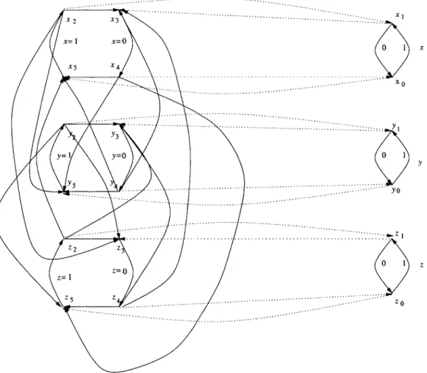
2.2.1 The Construction

Given a set of m linear equations on n variables, we construct a graph G using the following rules: (We assume all equations have the right hand size zero by negating one literal if necessary.)

1. For each variable x E F, we create two vertices and two edges. The vertices are xO and x, and the edges are (xi, xo) and (xo, xi). These vertices and edges will form the

variable gadget.

2. For each clause Cj E F, we add the clause gadget. The clause gadget is shown in Fig-ure 2-2. For a literal x in the clause we create a 4-cycle {X2, X3, x4, X5}. We label edge

Then we add the following 12 edges: (z2, X5), (z2, Y3), (z4, y3), (z4, x3), (x2, z3), (X2, Y5), (X4, ZO), (X4, YO), (W2, Z3), (Y2, ZO), (Y4, X3), (W4, X5)

3. We connect each clause gadget to the corresponding variable gadgets in the following way: For a literal x, we connect the corresponding 4-cycle in the clause gadget to the variable gadget by adding edges (x2, X1), (X1, X 3), (XO, X5), (X4, xo). The idea is that

an edge in the clause gadget that corresponds to a variable x being set to 1 (labeled

x = 1 in Figure 2-2) should be in a cycle with the edge in the variable gadget that

corresponds to the variable being set to 0 (labeled 0 in Figure 2-2), so that one of these edges is removed and the settings of the variable is determined by the remaining edge. Since all clauses are connected to the same variable gadget, this will maintain consistency in the variable assignments of each clause.

The resulting graph G has 36m + 2n edges, 36 for each clause gadget and 2 for each variable gadget. In order to relate variable assignments to acyclic subgraphs of G, we will say removing the edge (xi, xO) corresponds to setting the variable x to true, and removing the edge (xo, xi) corresponds to setting the variable to false.

2.2.2 The Proof

We will use another theorem of Histad for this proof:

Theorem 3 (Histad [6]) For every e > 0, it is NP-hard to tell if a given a set of linear

equations modulo 2 with 3 variables is satisfiable or at most m(-! + e) of its clauses are satisfiable.

Lemma 5 The minimum feedback arc set for the graph G contains n + 3m + u edges, where u is the minimum number of unsatisfied equations.

Proof. By Lemma 1, exactly one edge from every variable gadget is in the minimum feedback arc set. In addition, we need to show the following things:

(i) Given a clause, x + y + z = 0, and an assignment that satisfies this clause, we will need to remove only three edges from the corresponding clause gadget so that the subgraph consisting of the clause gadget and it three corresponding variable gadgets is acyclic. There are four assignments to the variables x, y, z that satisfy this clause. They are: {{0, 0, 01,

{0, 1, 1}, {1, 1, 0}, {1, 0, 1}}. We need to show that for any one of these assignments, if we remove the three corresponding edges, then the subgraph of the remaining edges from the clause gadget and relevant variable gadgets is acyclic.

First, note that any cycle in a clause gadget must contain labeled edges. This is because for every non-labeled edge (i,

J),

i is a vertex such that the only incoming edge is a labeled

edge, and

j

is a vertex such that the only outgoing edge is a labeled edge.

We now consider the four possible satisfying assignments for the clause x + y + z = 0:

1. {x = 0, y = 0, z = 0}. This means that all edges in Figure 2-2 labeled x = 1,y =

1,z = 1 are removed. The three edges labeled x = 0, y = 0, z = 0 are not in a cycle together. If they were, vertex X4 would have to be in a cycle, but all four of its out

edges lead to edges labeled 1, which are removed. Thus, the remaining set of edges is acyclic.

2. {x = 0, y = 1, z = 1}. Then the edges labeled x = 1, y = 0, z = 0 are removed. The remaining graph is acyclic, since if you consider the four edges going out from the edge labeled z = 1, all four of these edges lead to a vertex whose only out edge has been removed.

3. {x = 1, y = 0, z = 1}. Then the edges labeled x = 0, y = 1, z = 0 are removed. If

we consider vertex X2, which is the endpoint of the edge labeled x = 1, all four edges lead to vertices whose only out edge has been removed. So the remaining set of edges is acyclic.

4. {x = 1, y = 1, z = 0}. We remove edges x = 0, y = 0, z = 1. Consider vertex z4,

which is the endpoint of the edge labeled z = 0. All four edges leaving this vertex lead to vertices, whose only out edge has been removed. So the remaining set of edges

is acyclic.

(ii) Given a clause, x + y + z = 0, and an assignment that does not satisfy this clause, we will need to remove exactly four edges from the corresponding clause gadget so that the subgraph consisting of the clause gadget and its three corresponding variable gadgets is acyclic. There are four assignments to the variables x, y, z that do not satisfy this clause. They are: {{1, 11}, {0, 0,1}, {1, 00}, }{0, 1, 0}}.

1. {x = 1, y = 1, z = 1}. Then the edges labeled x = 1, y = 1, z = 1 remain and form a cycle. So we must remove one of these edges and the remaining graph is acyclic. 2. {x = 0, y = 0, z = 1}. Then the edges x = 0, y = 0, z = 1. These edges are in a cycle,

so, again, we must remove of four edges.

3. {x = 1, y = 0, z = 0}. Then the edges x = 1, y = 0, z = 0 remain and create a cycle, so we must remove four edges.

4. {x = 0, y = 1, z = 0}. Then the edges x = 0, y = 1, z = 0 remain and form a cycle, so we must remove four edges.

(iii) For each variable gadget, if we remove one of the two edges and the correspond-ing edge from the clause gadgets representcorrespond-ing clauses that contain this variable, then the remaining graph does not contain any cycle composed of edges from more than one clause gadget. For the clause x + y + z = 0, consider the edge (X2, X1). If a cycle contains this edge, it must also contain the only incoming edge to vertex X2, which is the edge labeled

x = 1. If these edges are contained in a cycle with edges from another clause gadget, then at vertex x1, we can move to another gadget. However, we will arrive at a vertex such that

the only out edge corresponds to the edge that remains iff x has been set to 0, which is not the case if the edge labeled x = 1 was present. So there cannot be any cycles that use edges from more than one clause gadget.

It follows from (i),(ii), and (iii) that the minimum feedback arc set has size n+3m+u.EJ

Corollary 6 The Maximum Acyclic Subgraph for G is of size n + 33s + 32u where s and

u represent the number of satisfied and unsatisfied clauses, respectively, for an assignment that satisfies the maximum number of clauses.

Theorem 4 The maximum acyclic subgraph can not be approximated to within 5 for any

e > 0.

Proof. By Corollary 6 and by Theorem 3 it is NP-hard to distinguish between a graph that has a maximum acyclic subgraph of size n + 33(1 + E)m + 32(1 - c)m and a graph that

has a maximum acyclic subgraph of size n + 33m. If we could approximate the maximum acyclic subgraph to within 6+ , then we could distinguish between these two cases. Therefore it is NP-hard to approximate to approximate the maximum acyclic subgraph to within 2 +e. We can make n arbitrarily small compared to m by creating another set of linear equations in which each original equation appears k times for some k so that we have

km clauses and only n variables. The ratio 2n+65 _2n+66 is arbitrarily close to 2 as k becomes₆₆ large. Therefore, it is NP-hard to approximate the maximum acyclic subgraph to within

... ... _{I... ... _} x 2 X 3 ... X= I X=o 0 1 x X5 X4 ... .. ... ... ... ... ... .. ... .... .. * ... ... X o ... ... ** ... ... ... ... .... _{... ... ... ...} ... ... Y 1 Y3 Y= Y=O 0 1 y Y 5 .... ... 11 ... ... ... . YO . ... _.* ... ... ... ... _{... ... ...} ... .. _{... ...} ... _{.... ... .. ... .. .. ... ... ... ....} - .0- Z .... Z 2 z 0 1 z 1 Z=O Z 5 z 4 ... ... Z O ... ... ...

Chapter 3

Linear Programming Relaxations

In this chapter we discuss linear programming relaxations for the maximum acyclic subgraph problem.

3.1

Two Integer Programs

The maximum acyclic subgraph problem can be viewed as maximizing the number of edges subject to a constraint for every cycle. The constraint specifies that the sum of the edge variables on a cycle of length C is at most

1C

- 1. These constraints are described by the following integer program:

maximize _{EijEE Xzi} subject to:

jeczg 10 - 1

VijEE Xij E {O, 1}

It is NP-hard to solve this integer program. However, we can relax the requirement that xii are in {0, 1} and replace it with the requirement that that 0 < xi < 1. We can solve the resulting linear program in polynomial time using the Ellipsoid Algorithm because it has the following polynomial separation oracle [5]. Given a solution to the linear program, we can consider the graph with each edge (i,

j)

assigned weight 1 - xij. Then we can find

the minimum weight cycle. If there is any cycle that has weight less than 1, then we have found a cycle with value more than

IC

- 1 which is a violated constraint. We refer to this linear program as LP1.

Another integer program for the maximum acyclic subgraph problem has a variable for every pair of vertices i, j E V. In this program, there are only constraints for 2- and 3-cycles: maximize _{EijEE Xii}

subject to:

Vi~j Xij + Xji=1

Vi,j,k Xij + Xjk + Xki

<

2

Vi~j Xij E to, 1}

Lemma 7 An integral solution to the above integer program represents an acyclic subgraph. Proof. Consider some acyclic subgraph S C E that includes every edge which is assigned a 1 by this integer program. If each 2-cycle in the complete directed graph has at most one edge S and each 3-cycle has at most two edges in S, then we prove by induction that every

cycle of length

JCJ

;> 4 has at most

IC!

- 1 edges in S.

Consider a 4-cycle {V1, V2, V3, V4}. Choose two non-adjacent vertices v, and V3 on the

4-cycle. Consider the 2-cycle that connects these two vertices. One of these edges is in S, say (v₃, vi). Then we cannot include both (vi, v2) and (v2, v3) in S, so at most three edges from

this 4-cycle are in S. Similarly, assume each cycle of length at most C contains at least one edge assigned 0 by the integer program. Then consider some cycle x = {V1, v2, -. , Vc+1}

of length C + 1 and choose any two non-adjacent vertices on the cycle, vi and v3. Consider

the 2-cycle that joins these vertices. One of the edges, say (vi, vj) is in S. Since the cycle

{vi, vj, vj+1I, - * vi_} has length at most C it follows that at least one of the edges in x on

the path from xj to xi is assigned 0 by the integer program. Therefore, we can include at most C edges from a cycle of length Cl +1 in S.

Again, it is NP-hard to solve this integer program. However, we can solve the relaxation in polynomial time using the Ellipsoid Algorithm because there are only a polynomial number of constraints [5]. We will refer to this relaxation as LP2.

3.2

Linear Program Integrality Gap

The integrality gap of a linear program is defined as the ratio of the size of the optimal integer solution to the size of the optimal fractional solution returned by the linear program. It is not known how to use a linear program to obtain an approximation ratio that is better than the integrality gap. In this section, we will show that the integrality gap for both LP1 and LP2 is 2 implying that these linear programs will not lead to a better-than-half

approximation algorithm. As a basis for the construction, we will use the fact that there exists a class of undirected graphs with girth g and E(n -(Q) ) edges. (See Section 3.3 for the construction.)

Given such a graph G with girth -log n (we could use any function that is o(log n) for the girth), we will show that the following lemma holds:

Lemma 8 There exists at least one directed orientation of G such that for any ordering of

the vertices, the number of back edges is at least (1 - e) 1E1 for any e > 0.

Proof. For any E > 0, we show that with non-zero probability, a directed orientation of G has at least (1 - c) ! back edges for any ordering of the vertices where m is the number of edges in G, i.e. the size of its maximum acyclic subgraph is very close to half the edges. For this proof, we use a Chernoff bound found in [9]:

Theorem 5 Let X1, X2, --, X, be independent Poisson trials such that, for 1 < i < n,

Pr[Xi = 1] = pi, where 0 < pi < 1. Then, for X = J_1 Xj, it = E[X] = n 1 pi, and 0 < j < 1,

Pr[X < (1 - 6)p] < e- 2

We fix an ordering of the vertices and we choose a directed orientation of G at random. For each edge (i, J), we direct the edge from i to

j

with probability 1 and from j to i with probability 1. Thus, each edge is a forward edge or a backward edge with equal probability. We associate an indicator random variable Xi with the ith edge so that Xi is 1 if the ith

edge is a backward edge and 0 if it is a forward edge in this ordering. Thus, for all Xj,

p= . X is the random variable that represents the number of back edges and A = !, i.e.

the expected number of back edges for a fixed ordering of the vertices is !. Using Theorem 5, we find that:

m2 Pr[X < (1 - c) ] < e 4

In words, the probability that a particular directed orientation of the edges with respect to a fixed ordering of the vertices has less than (1 - e)' back edges is exponentially small in

m for any e > 0.

Now we fix the orientation of the edges and show that with non-zero probability this directed graph has close to ' back edges for every ordering of the vertices. There are

n! < 2' log orderings of the vertices. By union bound, the probability that this directed

graph has less than (1 - E) M back edges for at least one ordering of the vertices is:

< e- 42"I

If this quantity is < 1, then the probability that a particular orientation of the edges has at least (1 - E) M back edges for every ordering of the vertices will be > 0.

m2

If e--4 2"logn < 1, then taking the log of each side, we have:

mE 2 me2 4nlogn

4+ nlogn < 0 = nlogn < E > m

~>

When g = Vlogn, we need to show that E is o(1). Then for any fixed e > 0, this inequality

1 _________3

will be true for large enough n. Since (g)Vgn- = 2 ' -Viig and logn = 211ogogn and

log log n < Vlogn - (since log x < f - ), we have E = o(1). Thus, with non-zero probability, there is some directed graph with girth -log n that has a maximum acyclic

subgraph of size (1 - E)i-[ for any e > 0. L

We will refer to a directed graph on n vertices with girth Vlog n and maximum acyclic subgraph of size at least (1 - E) as G*. We will use G* to prove the following lemmas: Lemma 9 The integrality gap of LP1 is 2.

Proof. For any e > 0, we can find an n such that G* has an maximum acyclic subgraph of size at least (1 - e)M. Since G* has girth at least Vlog n, a feasible solution for LP1

is to assign each edge in E the value (1 - ) Thus the solution of LP1 has size at

least

IEI(1

- _logn ). The ratio of the optimal solution to the optimal fractional solution is

hog *. As e decreases, n increases. Thus, lim n+ -- = 2. Since this ratio can be

made arbitrarily close to 2 for large n, the integrality gap is 2. 0

Lemma 10 The integrality gap of LP2 is 2.

Proof. Given a maximal solution to LP1 for a graph G, we can construct a solution to

LP2 for G with the same objective value. A solution to LP1 includes an assignment for

every edge in G. The solution we will construct will contain an assignment for every pair of vertices i, j

C

V. Let x be the maximal solution given for LP1.

We extend the solution x as follows: for all (i, J) E E, (j, i) ( E, we assign xji = xij.

Now every cycle in x of length |CI has total value at most C| - 1. This is equivalent to saying that every cycle has total value at least 1, since if some cycle has total value less than 1, then the cycle composed of the complementary edges must have total value more than |C - 1. This is clearly true of all cycles in E. Let E be the set of edges that are not in

E but whose complements are in E whose values we just added to x. Then all the cycles in

E

must also have total value at most IC - 1. If this were not the case, then some cycle in

E would have value less than 1, which means the solution x is not maximal. The last case

we need to consider is a cycle composed of edges from both E and E. Let A be the edges in this cycle from E and a denote their total value and let B be the set of edges in this cycle from

E

and b denote their total value. Assume a + b > |C| - 1 where A and B form cycle

The edges in R are in E and x is maximal. This means that there must be some cycle C' in E containing B such that the set of edges C - B has total value

IC'I

- 1 - L and the set of its complementary edges has value L. These complementary edges form a cycle with the edges in A which has value U. Both sets are in

E

which implies that d + L> 1.

Therefore, all cycles in x have total value at most

1C

- 1 and at least 1 so x is still a valid solution to LP1. For each pair of vertices i, j E V such that (i, j) and (j, i) are not

in E, the inductive step will be to show that we can find an assignment for xij and xji

such that the resulting x is still a solution to LP1 for the graph G + (i, j). Thus, when we

have assigned values to all pairs of vertices not associated with edges in E, we will have a solution for LP1 for the complete graph. This must also be a valid solution to LP2 since

if every cycle has value at most

1C

- 1 then every 2- and 3-cycle in the complete graph complies with the constraints in LP₂.

Now we prove the inductive step: to add an assignment to x we choose a pair of vertices

i,

j

that are not connected by an edge in G. Let a be the length of the shortest path from

i to j and 8 be the length of the shortest path from

j

to i. Together these shortest paths

form a cycle in G. Therefore a +

/

is at least 1. We let edge (j, i) have value xji = max {0, 1 - a} and edge (i, j) have value xij = min {1, a} = 1 - xji. If a > 1, then any cycle

that includes edge (j, i) has total value at least 1 and edge (i, j) has value 1 so any cycle that includes edge (i, j) has total value at least 1. If a < 1, then any cycle that includes edge (j, i) will have total value at least 1 and every cycle that includes edge (i, j) will have total value at least a +

#,

which is at least 1.

Since we can construct a solution for LP2 with the same objective value as LP1 so the

integrality gap for LP2 must be the same as LP1.

3.3

Constructing Undirected Dense Graphs with High Girth

In this section, we present a proof of a lemma that is due to Erdos and Sachs [10]. Lemma 11 There exist undirected graphs with girth at least g and E(n - (11) g) edges. Proof. We will construct a graph with girth g and E(n -

(Q)

) edges. First, we construct

a graph on n vertices by choosing d perfect matchings in Ka a uniformly at random. Since each vertex has degree at most d, then for some vertex v there are at most d9 paths of length g that begin at this vertex. We will set d9 = ! (we will solve for d later). If we take a random walk of length g starting from vertex v, then the probability that we return to vertex v sometime during the walk is the number of vertices that we reach-at most dg-divided by the total number of vertices in G. Since d9 = , the probability that we return to vertex v after taking at most g steps is =

}.

We will now use the Chernoff bound defined in Section 3.2. For each vertex, we can define an indicator random variable Xi. Let Xi = 1 denote that there is no cycle of length less than or equal to g that contains vertex i and let Xi = 0 denote that there is some cycle of length at most g that contains vertex i. Then pi = 1 for all i. X is the random variable representing the total number of vertices included in cycles of length less than or equal to g and p = Z. By Theorem 5, we have:

,2 7

Pr[X < (1 - E) < e

9]

For any fixed E, this is very high probability, so we can assume that we have extremely close to 27a vertices that are not contained in cycles of length less than or equal to g. The remaining set of 1 vertices may be contained in cycles of length less than or equal to g, but we can remove these vertices and all edges adjacent to them. This entails removing no

d, dn, 3dn

more than 1 edges, so we are left with 2 - 8 edges.

Now we solve for d: d9 = , so d = . Therefore

El

= d = ( So we have found a graph with E(n-

())

edges and girth at least g. l

Chapter 4

Restricted Problem

In this chapter, we investigate the maximum acyclic subgraph problem restricted to certain classes of graphs, namely Eulerian graphs and graphs with maximum degree 3. Somewhat surprisingly, the general problem can be reduced to these special cases. First, we present an approximation-preserving reduction from the maximum acyclic subgraph problem in general graphs to the maximum acyclic subgraph problem restricted to Eulerian graphs. Then we use this reduction to give an approximation-preserving reduction from the maximum acyclic subgraph problem in general graphs to the maximum acyclic subgraph problem in graphs with maximum degree 3.

4.1

Eulerian Graphs

This reduction is due to Liazl6 Lovaisz and Fang Chen [8].

Theorem 6 If for any 6 > 0, there exists a (1

+

6)-approximation algorithm for the maxi-mum acyclic subgraph problem in Eulerian graphs, then there exists a (I + )-approximation algorithm for the maximum acyclic subgraph problem in general graphs.

Proof. We will say a graph G is e-far from Eulerian if there is a v E V for which d+(v) or d-(v) > (I + E)d(v). If 4E > 6 z 6 > , then we can make at least an 6 (or ) gain at

each vertex (by placing the greater of the in and out edges in the acyclic subgraph) until the graph is less the -far from Eulerian.

If 4c < 6 = E < _4,, we will add a new vertex v* to G to obtain a new graph G + v*. To the vertex v* we will attach in edges and out edges from and to each vertex in G for which Id+(v) - d-(v)I > 0, thus making G + v* Eulerian. Let OPT(G) denote the size of

d(v*) -

S

|d+(v) - d-(v) |

5E

2ed(v) < 2e

5

d(v) < 4c|E| 4EOPT(G)

vEG vEG vEG

If we have a

(j

+ 6)-approximation for G + v*, then:

OPT(G + v*) > OPT(G) + -d(v*) => OPT(G + v*) - d(v*) >

+ 6)OPT(G + v*) - d(v*) >

(1 + 6)OPT(G) +

(1

+6)!d(v*) - d(v*) >

(

+6)OPT(G) - d(v*)> (! +6)OPT(G) - 3EOPT(G) >

(!

+6- 3E)OPT(G)

Since 4e <6 = E <

1 1 3 16

(- + 6 - 3e) > (- + 6 -- 6) = (- + -)

2 2 4 2 4

So we can get a (1+ )-approximation algorithm for all graphs given a (1+6)-approximation

algorithm for Eulerian graphs. L

4.2

Degree-3 Graphs

The maximum acyclic subgraph problem remains NP-hard even for graphs with maximum degree 3 [7]. (For graphs with maximum degree 2, the problem is easy.) In this section, we give an approximation-preserving reduction from the maximum acyclic subgraph problem for Eulerian graphs to the maximum acyclic subgraph problem for graphs with maximum

degree 3.

Theorem 7 If for any E > 0, there exists a ({ + e)-approximation algorithm for the

maximum acyclic subgraph problem in graphs with maximum degree 3, then there exists some 6 > 0 such that there is a (I + 6)-approximation algorithm for the maximum acyclic subgraph problem in general graphs.

To prove this theorem we will first introduce the following lemmas.

Lemma 12 Given an Eulerian graph G = (EG, VG) we can construct a 3-regular graph

G' = (EG', VG') with |EG| = 9|EGI - 91 G\ such that the size of the minimum feedback arc set in G is the same size as the minimum feedback arc set in G'.

Proof. Since G is Eulerian, we will use d(v) to denote both the in- and out-degree of

vertex v for this proof. The figure below shows a vertex v in G before we add any vertices or edges.

V

The construction of G' is as follows: we first place a vertex in the middle of each edge of G.

The number of vertices is now IVGI + IEGI. Then for each vertex v E VG, we match each incoming edge with a distinct outgoing edge by adding an edge from the vertex placed on the incoming edge to the vertex placed on the outgoing edge. (Since G is Eulerian, we will always be able to find such a matching.)

All of the IEGI new vertices now have in- and out-degree 2. We want to replace the vertices from VG with a new set of vertices in which each vertex has in- and out-degree 2 so that the entire graph will be 4-regular and Eulerian. Consider vertex v E VG. We build a binary tree from v to the d(v) new vertices placed on the outgoing edges.

This requires d(v) - 2 new vertices. We can see this by the following reasoning: let p be the highest power of 2 not greater than d(v). For a binary tree that connects p vertices to v, we need R + P +. .+ 2 = d(v) - 2 new vertices or vertices that are internal nodes on the

binary tree. For each of the remaining d(v) - p vertices, we will connect two vertices to one of the p leaves thus adding just one internal vertex for each of these vertices. Therefore, we have a total of d(v) - p + p - 2 = d(v) - 2 internal or new vertices on the binary tree.

We also build a binary tree from v to the d(v) new vertices placed on the incoming edges. Then we match each vertex from the incoming binary tree with a distinct vertex from the outgoing binary tree by adding an edge from the former to the latter.

V4

We build these two binary trees and match their vertices as we just described for all vertices " E VG. The total number of new vertices needed to build these two binary trees for vertex

v is 2d(v) - 4. The total number of new vertices needed to build two binary trees for all

v C VG is therefore

Z

VG 2d(v) - 4 = 21EGI - 4

1VG.

We now have a 4-regular Eulerian graph with (lEG! + IVGI) + (21EGI - 41 VG) = 3IEG I

31VGI

vertices. We are not yet finished constructing G' since we want G' to be a 3-regular graph, but we will call this intermediate graph G". The last step in the construction of G'

is to stretch each vertex in the current graph into an edge so that G' is 3-regular.

After the final step in the construction of G',

IEG'I

= 3(3|EGI - 3|VG|) = 9|EGI - 91VG .

We will use the following definition later on in the proof.

Definition 1 A blue edge is an edge (i,j) such that vertex i has in-degree 2 and vertex j

has out-degree 2.

Note that the edges in G' that correspond to vertices in G" are blue edges.

We will now show that this reduction preserves the size of minimum feedback arc set, i.e. the size of the minimum feedback arc set of G' is equal to the size of the minimum

feedback arc set of G. Specifically, we will show that given a feedback are set in G, we can construct a feedback arc set in G' of the same size. Conversely, given a feedback arc set in G', we can construct a feedback arc set in G of size at most the size of the feedback arc set in G'.

(i) Suppose F is a feedback arc set of G. We will construct F', a feedback arc set of G'. For each edge eij E F, we add to F' the blue edge from EG' that corresponds to the vertex used to subdivide edge eij in the first stage of the construction of G'. Then

IF'I

= |F and

EG' - F' is acyclic by the following proof.

Assume EG' - F' is not acyclic. Note that every blue edge corresponds to an original

edge, to an original vertex, or to a vertex on a binary tree in G". If we take a walk on the graph G' starting from a blue edge corresponding to an edge eij in G (i.e. to a vertex used to subdivide an edge in the first step of the construction) we will either follow a path on the binary tree leading to a blue edge corresponding to edge ejk or we will walk directly to edge ejk for some k. Therefore, if we find a cycle in G', the set of edges in that cycle that correspond to edges in EG are still present in G implying that there is a cycle in G, which is a contradiction to the fact that F is a feedback arc set.

(ii) Suppose F' is a feedback arc set in G'. Assume all edges in F' are blue edges. If they are not, we can replace them with blue edges adjacent to the non-blue edges and obtain a feedback arc set of equal or smaller size. Then for every edge in F' that corresponds to an edge in EG, add the corresponding edge in EG to F. Then EG - F is acyclic by the

following proof.

Assume EG - F is not acyclic. Then consider some cycle in EG - F. The blue edges

corresponding to each edge eij in the cycle are still in EG' - F'. Since EG' - F' is acyclic,

at least one of the edges used to connect vertices that we placed in the middle of the edges in EG must have been removed. But this is a contradiction, because these edges are not blue edges, and we converted F' to a feedback arc set that contained only blue edges. l

Corollary 13 A maximum acyclic subgraph in G of size S corresponds to a maximum

acyclic subgraph in G' of size S + 8IEGI - 91VG1.

Proof. Given a maximum acyclic subgraph in G of size S, we can find a feedback arc set in G of size EG - S. Therefore, we can find a feedback arc set in G' of size EG - S.

There will be S + 81EGI - 9 VG| edges remaining in EG' and these edges make up an acyclic subgraph of G'.

Lemma 14 We can convert an acyclic subgraph of G' of size at least (i7 + C)MAS(G') to

Proof. Let MAS(G) denote the size of the maximum acyclic subgraph of G. We assume that MAS(G) is at least

#EG

for some fixed

#

< 1 (we will explain

#

later). If MAS(G) is less than 3EG, then we can find an acyclic subgraph in G with at least half the edges of G thereby obtaining a (I + e)-approximation for some c > 0.

Say we are given an a-approximation algorithm for 3-regular graphs. We can take an Eulerian graph G and convert it a 3-regular graph G' using the construction described previously. Then we can find an acyclic subgraph S' for G' that is of size at least aMAS(G'). By Corollary 13 we have:

aMAS(G') = a(MAS(G) + 8EG - 9VG)

To find an acyclic subgraph S of G given S', we remove all edges from S' that do not correspond to blue edges representing original edges of G. There are at most 8EG - 9VG

such edges, since EG of the edges in G' correspond to edges in G. So when we remove these edges from S', we are left with a set S of size at least:

a(MAS(G) + 8EG - 9VG) - (8EG - 9lG) = aMAS(G) + (8a - 8)EG + (9 - 9a)VG

Since EG MAS(G) ______ 8a - 8 < 0, and VG > MAS(G) where d is the average degree of

G, we have:

aMAS(G) + (8a - 8)EG

+

(9 - a)VG >! OMAS(G) + (8a - 8) AS(G) + (9 - 9- ) MAS(G)

And:

a8±+>9 8a 8 1 8a > 1 8

Since 8 < 1:

a > (0+16) 1 17

(0+8) 2 18

Therefore, if we found a (1 +6)-approximation for 3-regular graphs, then we could find some

3

such that the above inequality is true. If MAS(G) >

#EG,

then we could use the reduction and the (}Z+ 6)-approximation algorithm for degree-3 graphs to find a (1+e)-approximation for Eulerian graphs, which would by Theorem 6 lead to a (I + {)-approximation for general

graphs. E

Theorem 8 There is no PTAS for the maximum acyclic subgraph in degree-3 graphs unless P = NP.

Proof. If we have an a-approximation for the maximum acyclic subgraph in degree-3 graphs, then we will get a (a + 8(a-1) )-approximation for Eulerian graphs. Therefore, if a=1-E andifB > -, then:

a + 8(a-1)- > - 17c

Thus, if we can find a (1 - E)-approximation for the maximum acyclic subgraph in degree-3 graphs, then we can find a (1 - 6)-approximation for Eulerian graphs, where 6 = 17E, which implies that we can find a PTAS for Eulerian Graphs. This implies that we can find a PTAS for general graphs, which is a contradiction, since the maximum acyclic subgraph problem for general graphs does not admit a PTAS. (See Chapter 2 for a proof of this.) E

Chapter 5

Algorithms for Degree-3 Graphs

In [1] an algorithm that returns an acyclic subgraph of size i E| is given for graphs with maximum degree 3 and an algorithm that returns an acyclic subgraph of size 1}lE is given for 3-regular graphs. In this chapter, we show that the maximum acyclic subgraph problem in graphs with maximum degree 3 can be approximated to within of optimal using simple combinatorial methods.

5.1

Assumptions

Given a graph G with maximum degree 3 for which we want to find an acyclic subgraph S, we can assume the following in any algorithm:

(i) All vertices have total degree exactly 3. If there is any vertex v such that d+ (v) =

d-(v) = 1, then we can remove the vertex and treat the adjacent edges as one edge. Thus

an edge in the modified graph may represent a path in the original graph. If we ever add an edge representing a path to S, then we are really adding all the edges in the path to S. If we do not add this edge to S, then we can remove any one edge from the path and add the rest of the edges on the path to S. If for any vertex d+(v) = 0 or d-(v) = 0, we can add all edges adjacent to v to S.

(ii) G has no 2- or 3-cycles, since we can treat both optimally. For 2-cycles, consider the 2 adjacent non-cycle edges. If they are both in edges, or both out edges, then we can break the two cycle by removing an arbitrary edge. If one is out and the other is in, then one of the edges in the 2-cycle is consistent with the direction of a possible cycle containing both of the two non-cycle edges, so we can remove this edge. For 3-cycles, if we contracted the 3-cycle, we would get a new vertex of degree 3. If this vertex is a source or a sink, then we can remove an arbitrary edge from the 3-cycle. Otherwise, we remove an edge from the 3-cycle, so that the path to or from the single in or out edge is broken.

5.2

Algorithm 1

We will now consider the case where G has no blue edges. See Section 4.2 for the definition of a blue edge. If there are no blue edges, then we can find the maximum acyclic subgraph

in polynomial time. For our algorithm, we will use the following lemma:

Lemma 15 If G has maximum degree 3 and contains no blue edges, then all cycles in G

are edge disjoint.

Proof. Assume that there are some 2 cycles in G that have an edge (or a path) in common. First case: assume that these two cycles have an isolated edge (i,

j)

in common, i.e. edge (i, j) belongs to both cycles, but edges (a, i) and (j, b) each belong to only one

of these cycles. Then vertex i must have in-degree 2 and vertex

j

must have out-degree 2. Thus, edge (i, J) is a blue edge, which is a contradiction. Second case: assume these two cycles have a path {i, - - -, j} and that this path is maximal, i.e. edge (a, i) and (j, b)

each belong to only one of these cycles. Vertex i must have in-degree 2 and vertex j must have out-degree 2. Therefore, one of the edges on the path must be a blue edge, which is a

contradiction. E.

Since all the cycles in a graph with no blue edges are edge disjoint, we can find the maximum acyclic subgraph of such a graph in polynomial time. Given a graph G containing no blue edges, the following is an algorithm to find the maximum acyclic subgraph of G: Algorithm 1: Step 0. Step 1. Step 2. Step 3. Let S={},G'=G.

While G' is not acyclic, do:

Step la. Find a cycle in G'.

Step 1b. Remove an edge in this cycle from G'.

Step 1c. Remove the rest of the edges in this cycle from G' and

add them to S.

Add the remaining edges to S. Output S.

5.3

Algorithm 2

If G has blue edges, then the problem is NP-hard. For this case, we will give the following

Algorithm 2:

Step 0. Let S={}, G'=G.

Step 1. While there are still blue edges in G', do:

Step la. Optimally treat any 2- and 3-cycles.

Step 1b. Find a blue edge e in G'.

Step 1c. If e is contained in a component with exactly 9

edges then:

Solve for the maximum acyclic subgraph of

this component exactly.

Else: Remove the four edges neighboring e from G'

and add them to S.

Step id. Contract any vertices with in-degree and out-degree 1.

Step 2. If G' is acyclic, then add all edges in G' to S. If G' is not

acyclic, then since it contains no blue edges, use

Algorithm 1 to find the maximum acyclic subgraph of G' and

add it to S.

Step 3. Uncontract every edge added to S that was contracted in Step

4. For every contracted edge that was removed from G' and

not added to S, remove any edge from the corresponding path

in G and add the remaining edges to S.

Step 4. Output S.

Theorem 9 Algorithm 2 is an -approximation for the maximum acyclic subgraph problem. Proof. _{We will show that for each iteration of Step 1 through Step 5 of the algorithm,} for every edge we remove, we contract or add to S a total of at least 8 edges. Edges that

we contract will be added to S in Step 3.

Consider a blue edge (i, j) in G. There must be four distinct vertices within distance 1 from i and j (since there are no 2- or 3-cycles). So there are 6 vertices that are at no more than one edge away from vertex i or vertex j (including vertices i and j). Therefore, there must be at least 3 = 9 edges in this neighborhood. If there are exactly 9 edges, then we have found a connected component and Algorithm 2 will solve this component exactly. Otherwise, if there are more than 9 edges in the neighborhood of edge (i, j) (i.e. there could be as many as 12 edges) then for each of the 4 distinct vertices that are exactly one edge away from i or j, we can either contract this vertex, or we can add two more edges to S (which would let us add more than 8 edges to S in this round). Thus, for every one

edge we remove from G, we add at least 8 edges to S which proves that Algorithm 2 is a

Bibliography

[1] Bonnie Berger and Peter W. Shor. Tight Bound of the Maximum Acyclic Subgraph Problem. In Journal of Algorithms, 25, pages 1-18, 1997.

[2] M. X. Goemans and L. A. Hall. The Strongest Facets of the Acyclic Subgraph Polytope are Unknown. In Proceedings of IPCO 1996, LNCS Vol 1084, pages 415-429.

[3] M. Gr6tschel, M. Jiinger, and G. Reinalt. On the Maximum Acyclic Subgraph Poly-tope. In Mathematical Programming, 33, pages 28-42, 1985.

[4] M. Gr6tschel, M. Jinger, and G. Reinalt. Facets of the Linear Ordering Polytope. In

Mathematical Programming, 33, pages 43-60, 1985.

[5] M. Gr6tschel, L. Lovasz, and A. Schrijver. Geometric Algorithms and Combinatorial Optimization Springer, 1988.

[6] Johan Histad. Some Optimal Inapproximability Results. In Proceedings of STOC,

1997.

[7] Richard M. Karp. Reducibility Among Combinatorial Problems. In Complexity of

Computer Computations, Plenum Press, 1972, pages 85-104.

[8] Laizl6 Lovaisz and Fang Chen. Personal communication.

[9] Rajeev Motwani and Prabhakar Raghavan. Randomized Algorithms. Cambridge Uni-versity Press, 1995.

[10] Dan Spielman. Applied Extremal Combinatorics Lecture Notes, Lecture 9, Fall 1998. Lecture notes available at: www-math.mit.edu/-spielman/AEC/notes.html.

[11] Vijay V. Vazirani. Approximation Algorithms. Preliminary draft of book available at: www.cs.gatech.edu/fac/Vijay.Vazirani.