Analysis and algorithms for parametrization, optimization and customization of sled hockey equipment and other dynamical systems

Analysis and Algorithms for Parametrization,

Optimization and Customization of Sled Hockey

Equipment and Other Dynamical Systems

by

Youzhi Liang

Submitted to the Department of Mechanical Engineering

in partial fulfillment of the requirements for the degree of

Doctor of Philosophy in Mechanical Engineering

at the

MASSACHUSETTS INSTITUTE OF TECHNOLOGY

February 2020

©Massachusetts

Institute of Technology 2020. All rights reserved.

Signature redacted

A u th or ...

Department of Mechanical Engineering

November 15, 2019

Certified by...

Signatureredacted

A.E. Hosoi

Professor/Associate Dean of Engineering

Thesis Supervisor

Signature redacted

~HUSSI...

OFTECHNOLOGY

_{NicolaA Hadjiconstantinou}

Chairman, Department Committee on Graduate Thesis

FEB 05

2020

10BRARIE

L S

MITLibraries

77 Massachusetts Avenue

Cambridge, MA 02139 http://libraries.mit.edu/ask

DISCLAIMER NOTICE

Due to the condition of the original material, there are unavoidable flaws in this reproduction. We have made every effort possible to provide you with the best copy available.

Thank you.

The images contained in this document are of the best quality available.

Analysis and Algorithms for Parametrization, Optimization

and Customization of Sled Hockey Equipment and Other

Dynamical Systems

by

Youzhi Liang

Submitted to the Department of Mechanical Engineering on November 15, 2019, in partial fulfillment of the

requirements for the degree of

Doctor of Philosophy in Mechanical Engineering

Abstract

A dynamical system, an ensemble of particles, states of which evolve over time, can be described using a system of ordinary/partial differential equations (ODEs/PDEs). This dissertation presents fundamental investigations of the analysis and algorithms for the study of dynamical systems, by parametrizing, optimizing and customizing. We develop and/or implement numerical algorithms, for solving ODEs/PDEs, and statistical/machine-learning algorithms based on data, for physical inference and pre-diction. We further apply the methodologies on sled hockey, an adaptation of stand-up hockey, allows people with physical disabilities to participate in the game of ice hockey.

First, we develop and implement numerical algorithms to study the nonlinear dy-namics described by 4th-order nonlinear PDEs. The non-linear solvers apply multi-dimensional Newton's method with a Jacobian-free approach and a generalized con-jugate residual (GCR) approach. Applying the algorithms on the study of elastic systems, we investigate dynamics of hockey sticks as in a striking implement. We develop a mathematical model using an Euler-Lagrange equation to characterize the behavior of a hockey stick in the linear regime, and then apply this model to in-vestigate the dynamic response of the stick throughout slap shots and wrist shots. We apply a modal decomposition method and decouple the resultant dynamics into kinetic and potential components. We further optimize the structures based on the dynamical analysis. Throughout testing with both elite and amateur sled hockey players, we find that final puck velocities with our prototype stick are on average over 10% higher compared to those achieved with commercially available sticks.

Second, we investigate the dynamics of rigid system as in an over-constrained implement. We propose two sets of dynamical modelling for the hockey sled using a trajectory-based modelling method and a state-space-based modelling method, which are used to study the dynamics of the propulsion for linear motion and of the tip-over and reset. We further propose a constrained optimization problem to optimize the

parameters of sled design and driving strategy to maximize the performance of sled hockey players based on the dynamics.

Third, we develop and implement statistical and machine learning algorithms based on data, including algorithms of clustering for physical inference, algorithms of regression for Stribeck curve and algorithms of forecasting for wear rate. In the context of tribology of ice-metal contact, we design an experimental system to mimic the ice rink environment and to expand the experimental study of the friction co-efficient in an extensive range of Hersey number from 101 to 10'. To build the understanding of the physics of friction, we perform a dimensional analysis and an asymptotic analysis for three regimes of friction - boundary friction regime, mixed friction regime, and hydrodynamic lubrication regime. We further develop a pipeline for creating the modified Stribeck curve based on data, after feature extraction, the regime of each experimental result is identified via clustering, followed by the regres-sion constrained by the asymptotic analysis. Finally, we propose a methodology and algorithm to predict the wear rate subject to geometric constraints.

Thesis Supervisor: A.E. Hosoi

Acknowledgments

I would like to express my greatest appreciation to my adviser, Professor Peko Hosoi, for her invaluable guidance, mentorship and inspiration, throughout my PhD program over the past four years. This dissertation has benefited greatly by her profound knowledge, in the areas of, amongst many others, structural dynamics, fluid dynamics, sports technology, algorithms and data science.

I thank my thesis committee members for their insightful feedback and guidance. I thank Professor Winter for his expertise on design for highly constrained environ-ments, machine and product design, and engineering global development; I thank Professor Yang for her expertise on system-level design for complex engineering sys-tems, early stage design process for products and syssys-tems, and design representation, including visual, physical and linguistic. Their advice and suggestions are extremely helpful and valuable for me.

I thank Mr. and Mrs. Greenberg for providing me with the opportunity of this research. I thank Wheelchair Sports Federation (WSF) New York Sled Rangers for their support on the surveys, interviews, experiments and insightful feedback for my research. WSF New York Sled Rangers are the Wheelchair Sports Federation New York Sled Rangers, serving as a sled hockey program for physically disabled youth with ages from five through twenty-one. They are one of the very few outlets for physically disabled kids to play competitive sports in New York City.

I thank Jordan Malone, a member of US Olympic Team for the 2010 Olympics, achieving numerous World titles including 2009 Men's Relay GOLD, for his insight of speed skating and design of skate blades and for his feedback on our study of the physics of ice friction.

I thank Josh and Max for the collaboration on the investigation of slap shots in sled hockey, especially for the co-authorship on the relevant publication. Thank Sarah for the collaboration on the investigation of wrist shots and for the co-authorship on the relevant publication. Thank Andrew for the collaboration on the development of numerical solvers for the dynamics of the Euler-Bernoulli beam and the relevant

publication. Thank Jose for the collaboration on the study of magnetorheological fluids and the relevant publication. Thank Bavand for his insightful input on the study of the friction coefficient between skate blades and ice and the relevant publication. I thank Yuanzheng, Kanghong, Zeyu and Jennifer for their review and feedback on this dissertation.

I thank all my teammates and alumni in Team Peko. The culture of Team Peko is dynamic, collaborative and inclusive. I thank Jose, Josh, Ben, Nathan, Alice, Jennifer, Juncal, Jean, Sarah, Kaitlyn, Audrey, Charlotte, Will and all the teammates and alumni not listed here. I thank Jose for his guidance on my study of fluid mechanics; I thank Kaitlyn for her help on the analysis of partial differential equations; I thank Nathan for his help on the electronics and control theory; I thank Josh and Ben for their help on the study of dynamics of systems; I thank Juncal for her help on the optimization methods. In particular, I thank Susan for always helping me out when I was in need.

I thank all the HML professors and labmates. The Hatsopoulos Microfluids lab-oratory (HML) focuses on the research on the dynamics of microstructures and mi-crofluidics, consisting of a single open-plan 6300 ft2 laboratory. The configuration

of the lab encourages collaboration between students with diverse backgrounds and expertise. During my MS and PhD program, I've received much help and support from the professors and labmates. I thank Professor McKinley for his expertise on extensional rheology of complex fluids and Non-Newtonian fluid dynamics; I thank Professor Bischofberger for her expertise on pattern formation and soft condensed matter. I thank Anoop and Jianyi for their instruction on the rheogology measure-ment and the corresponding customized devices. I thank Sean and Cakky for their service on the lab.

I thank my friends Yuanzheng, Kanghong, Hongyi, Qing, Jianyi. They are ex-tremely important to me. I very much value our friendship. I thank my friends for all their support and care for me. I thank Zhi, Shurui, Yongbin and Xiaoyu, Akira and Wenjun, Affi, Avani, Anthea, Borrelli, Liz, Shayan, Adam, Morgan, Sri, Tianshi, Xi-angming, Yulin, Dixia, Dayang, Yu, Bo, Yingyi, Ming, Shawn, Yili, Qingjun, Qifang,

Lei, Leixin, Lin, Chu, Haizheng, Quntao, Xiang, Wolski, Urmi, Morgan, Rachel, Ben, Caitlin, Thanasi, Jonathan, Sang, Jiuhong, Jianping, Jiheng, Lu and all the other friends not mentioned here.

I thank my parents and other relatives for their love, sacrifice and understanding, on the other side of the earth, for which I am forever grateful and more than I could ever hope to repay.

Contents

1 Introduction 29

1.1 What is Parametrization, Optimization and Customization . . . . 29

1.2 What is Dynamical System . . . . 30

1.3 Scope ofStudy .. . .... . . . .. . . . .. . . . .. . 31

1.3.1 Scope Identification . . . . 32

1.3.2 Outline of the Dissertation . . . . 35 2 Algorithms of Numerical Methods for Non-Linear PDEs

2.1 Background and Introduction . . . . 2.2 Algorithms of Numerical Methods . . . . 2.2.1 Algorithms of Numerical Solvers for Linear PDEs . . . 2.2.2 Algorithms for Numerical Solvers for Non-Linear PDEs 2.2.3 Algorithms for Reduced-Order Methods . . . . 2.3 Experiments, Results and Discussion . . . .

3 Dynamics of Elastic Systems - Slap Shots

3.1 W hat is Slap Shot ... 3.2 Dynamical Modelling and Parametric Optimization . . . .

3.2.1 Continuous Euler-Bernoulli Beam Model . . . . 3.2.2 Discrete Mass-Spring-Damper Model . . . . 3.3 Conclusion and Future Work . . . .

4 Dynamics of Elastic Systems - Wrist Shots

41 41 42 43 47 49 52 57 58 60 60 68 70 73

4.1 What is Wrist Shot ... 4.2 Dynamical Modelling and Parametric Optimization 4.3 Experiments, Results and Discussion . . . . 4.4 Conclusion and Future Work . . . . 5 Dynamics of Rigid Systems

5.1 Dynamical Modelling of Hockey Sled . . . . 5.1.1 Method 1: Trajectory-Based Modelling . . . 5.1.2 Method 2: State-Space-Based Modelling . . 5.2 Propulsion for Linear Motion . . . . 5.2.1 Kinematics and Dynamics of Propulsion . . 5.2.2 Parametric Optimization . . . . 5.3 Tip-Over and Reset . . . . 5.3.1 Dynamical Modelling of Tip-Over and Reset 5.3.2 Parametric Optimization . . . . 6 Tribology in Ice-Metal Contact

6.1 Background and Introduction . . . . 6.1.1 What is Tribology in Ice Friction . . . . 6.1.2 Stribeck Curve . . . . 6.1.3 Kinetic Friction of Ice . . . . 6.2 Dimensional Analysis . . . . 6.3 Experimental System . . . . 6.4 Asymptotic Analysis . . . . 6.4.1 Asymptotic Analysis for Elastohydrodynamic 6.4.2 Asymptotic Analysis for Mixed Contacts . . 6.4.3 Asymptotic Analysis for Boundary Contacts 6.5 Modified Stribeck Curve for Friction Coefficient . .

. . . . 74 . . . . 75 . . . . 79 . . . . 83 85 86 86 93 97 97 102 104 104 106 111 . . . . 112 . . . . 112 . . . . 114 . . . . 115 . . . . 117 . . . 118 . . . 120 Contacts . . . . 120 . . . . 121 . . . . 122 . . . . 125 7 Algorithms of Clustering for Physical Inference in Tribology

7.1 Feature Extraction and Feature Selection . . . .

127 127

7.2 Algorithms for Clustering Model . . . .

7.2.1 K-Means Clustering . . . .

7.2.2 Gaussian Mixture Clustering . . . .

7.3 Clustering for Physical Inference in Tribology . . . .

8 Algorithms of Regression for Stribeck Curve in Tribology

8.1 Background and Introduction . . . . 8.2 Algorithms for Statistical Model . . . .

8.2.1 Multi-Linear Regression . . . . 8.3 Algorithms for Machine Learning Model . . . . 8.3.1 Random Forest Regression . . . .

8.3.2 Neural Network Regression . . . .

8.4 Regression for Stribeck Curve . . . .

. . ... . 129 . . . . . 129 . . . . . 130 . . . . . 131 133 133 134 134 137 137 142 143 A Approval Letters from the MIT Committee on the Use of Humans

as Experimental Subjects (COUHES) 147

B Figures for Experimental Results in the Regime of Boundary

Fric-tion 151

C Figures for Experimental Results and Models in the Regime of

List of Figures

1-1 Survey results with 27 subjects, among which ten subjects are players, ten are parents, four are coaches and three are others. This survey is conducted to identify the stakeholder's needs and their priorities. (Inset) Results only for coaches. . . . . 34 1-2 Quality Function Deployment (QFD) analysis for the sled hockey project.

The customer requirements and technical requirements serve as the attributes and design parameters in QFD analysis, respectively. Ac-cording to the results from the interview and survey, we consider eight attributes and ten design parameters. The attributes are prioritized from 1 (top priority) to 8

(bottom

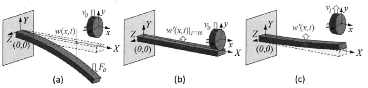
priority), based on the evaluation results for the relationships between the customer requirements and technical requirem ents. . . . . 36

2-1 (a) Cantilevered Euler-Bernoulli beam fixed at (0,0) with a Gaussian distributive load as function of space and time,

f(x,

t) = G1(x)G2(t).

We select the diamond point as the output point for the deflection of the beam. (b) Deflection of the loaded beam under external load as a function of space and time. . . . . 42 2-2 Transverse deflection of the beam in the form of discrete

representa-tion. (a) Free body diagram of each discrete element; (b) Discrete representation of a beam with N nodes . . . . 43

2-3 Deflection y (m) as a function of position x (m) for time t = 0.1 ins, t =

5 ms, t = 250 ms. The external load is a Gaussian distributive force in space, of which the center is located at x = 0.4 m. Trapezoidal integration method with a dynamically adjusted time step is applied. 44

2-4 Deflection at the center of the beam as a function of position x (m) subject to an impulse input force. The impulse force is modelled as a Gaussian distributive force with respect to time. The internal friction term in Eqn. 2.1 is taken into account in this simulation. . . . . 46

2-5 Deflection of a sled hockey stick under external load. (a) FEA simula-tion results using Solidworks with 289,959 DOF; (b) Simulasimula-tion results using our ID model. . . . . 46

2-6 Transverse deflection y

(m)

of the beam as a function of the position x

(m)

for the beam equation with/without the non-linear term. (a) Beam subject to a uniform distributed load. The external force b(x) is a constant. (b) Beam subject to a Gaussian distributed load. The external force b(x) is centered at x = 0.1. . . . . 48

2-7 Comparison of Bode plots of the transfer functions, using original sys-tem N = 500 and using reduced syssys-tem with q = 2 and 10 respectively (from left to right). The phase diagram appears to be shifted by 360 at some frequencies due to the plot setting using MATLAB by default. 51

2-8 Comparison of deflections of a sinusoidal response of the Euler-Bernoulli beam as a function of time, using original system N = 500 and using reduced system with q = 2 and 10 respectively (from left to right). . 51

2-9 (a) Bode plot for the original system and reduced system using mo-ment matching method. (b) Impulse response for original system and reduced system . . . . . 52

2-10 Histograms of the puck velocity for the rigid and flexible sled hockey sticks. Each histogram bar is normalized by the total number data points. (Inset) Percentage increase in puck velocity for each subject when using the flexible sled hockey stick. The dashed line indicates the average increase, 13.07 %. Subjects are shown in order of ascending percentage increase.. . .. .. .. . . . .. .. .. . . . .. .. .. . . 54 2-11 Puck velocity versus measured stick force for each subject. Linear

curves of best fit are shown as solid lines. The puck velocity for each point corresponds to the mean value across three trials, and the peak force for each players corresponds to the mean of five measurements. . 56

3-1 (a) Schematic of a stand-up hockey slap shot. (b) Schematic of a sled hockey slap shot using our prototype sled hockey stick. The flexibility is increased by using ABS plastic in place of wood. (c) Photograph of a sled hockey player using the conventional wooden sled hockey stick [1].

(Photograph credit John Freidah) The puck is highlighted in green. i: Backswing/Downswing; is: Stick preload; iii: Puck impact; iv: Puck release. . . . . 59 3-2 Schematic of our Euler-Bernoulli beam model of a sled hockey slap

shot. (a) Stick preload; (b) Puck impact; (c) Puck release. . . . . 60 3-3 (a)

#

plotted as a function of the Young's modulus of the beam

mate-rial, E. (Inset) The contribution of the first five mode shapes to the net value of 0. (b) Puck velocity V plotted as a function of the Young's modulus of the beam material. Solid and dash-dot lines correspond to the continuous and discrete models respectively. The colored dashed and dotted lines plot the contributions of the elastic and kinetic energy to the overall puck velocity (Vt and Vi, respectively). The shaded area highlights conditions where the stick deflection is large and our linear model may not be valid. . . . . 64

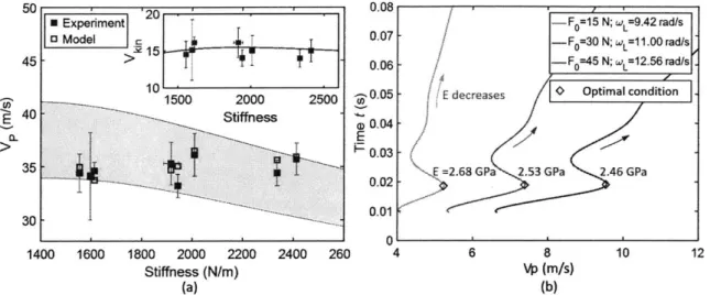
3-4 (a) We compare the predicted puck speed, V2 (m/s) of our model with

experimental data on stand-up slapshots over a range of stick stiffness values. Data is sourced from [2]. Within the the experimental data, the loading force varies significantly between shots. The shaded re-gion corresponds to predicted puck speeds V for the range of forces observed in [2]. (Inset) Vkj (m/s) plotted as a function of the stiffness (N/m). Vkj, is calculated by removing Vot from both the model and experimental puck velocities. (b) Time t (s) to perform a slap shot as a function of the puck speed V (m/s). Arrows indicate directions of decreasing Young's modulus E. The diamond markers delineate the optimal conditions labelled with the corresponding optimal Young's m odulus E . . . . . 65

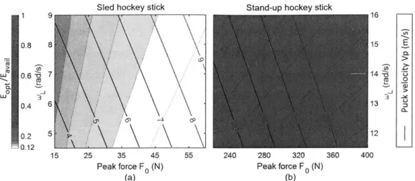
3-5 The ratio of the optimal Young's modulus of the stick material to the

available Young's modulus, Ept/Evai for sled hockey sticks (a) and for stand-up hockey sticks (b). The color map is in logarithmic scale. The ranges of the peak force FO for sled hockey and stand-up hockey are 15 N to 60 N and 230 N to 400 N respectively [2]; the ranges of the angular speed WL are 4.5 rad/s to 9 rad/s and 8.5 rad/s to 13 rad/s respectively [3]. . . . . 67

3-6 The ratio of the optimal Young's modulus of the stick material to the available Young's modulus, Ept/Evai for sled hockey sticks (a) and for stand-up hockey sticks (b). The color map is in logarithmic scale. The ranges of peak force FO for the sled hockey and stand-up hockey are 15 N to 60 N and 230 N to 400 N respectively [2]; the ranges of the angular speed WL are 4.5 rad/s to 9 rad/s and 8.5 rad/s to 13 rad/s respectively [3]. . . . . 68 3-7 (a) Discrete model. (b) Experimental setup. (c) Discrete model for

three stages of a slap shot. dyp/dt at t = t; and t = t+ are denoted as vo and vi respectively; dy,/dt at t = t; and t = t+ as no and ui

3-8 Comparison of theoretical and experimental mass displacements for our discrete collision model. (Inset) Theoretical results for the case of zero energy loss. . . . . 71

4-1 Schematic of the Euler-Bernoulli beam model for a sled hockey stick and a rigid body model for a puck.(a) Preload stage; (b) Release; (c) Post-Release stage. . . . . 75

4-2 Modal decomposition of initial deflection of the beam under static load. The first five eigenmodes are included in the figure. (Inset) Mode shapes of the first five eigen modes. . . . . 78

4-3 The magnitude of the puck velocity and the flexual rigidity as a

func-tion of Young's modulus of the material of the beam respectively. . . 79

4-4 (a) Prototype of a more flexible sled hoceky stick; (b) A commercially-available sled hockey stick. . . . . 80

4-5 _{Histograms for the magnitude of the velocity of the puck using two} types of sled hockey sticks. The histogram is normalized by the dis-crete probability density function (PDF). (Inset) The increase in per-centage of the magnitude of the puck velocity in ascendant order for each individual subject using flexible sled hockey sticks compared to that using rigid sticks. The dashed line indicates the average increase w hich is 11.48% . . . . . 81

4-6 The magnitude of the puck velocity versus the peak force that players can exert with two lines indicating the linear regressions using the two types of sled hockey sticks respectively. . . . . 83

5-1 Schematic of the frames and the trajectories for the motion of hockey sled. Point A is the contact point between the skate blade and ice surface. SA is the trajectory of A. Scoc is the trajectory of the center of curvature of SA. X1YZr is the inertial frame. Frame xyz is fixed on

the sled along the principal axis of the sled, of which the coordinates y and z locate in plane P2 and coordinate x in P1. Frame XYZ is an

intermediate frame, of which the coordinate y directs towards point A. P1 and P2 are virtual planes which are parallel and perpendicular to the curve SA respectively. . . . . 88

5-2 Schematic of the back view of hockey sled and free body diagram. N1 is the normal reaction force for the foot support of the hockey sled. Point A is the contact point between one hockey blade and the ice surface. N2 is the normal reaction force for skate blades at point A. bX/

and b, are distances between the center of mass and the foot support of the sled and point A respectively. F11 is the frictional force acted on

the skate blade. P2 is the virtual plane as shown in Fig. 5-1, which is

parallel to the trajectory of A. . . . . 89

5-3 Schematic of the back view of hockey sled and free body diagram. Point A is the contact point between one hockey skate blade and the ice surface. 0(t) is the lean angle of the sled, N2 is the normal reaction force

for the foot support and skate blade respectively. F1 is the frictional

reaction force between ice and the skate blade at point A. H, H and by are dimensions of the hockey sled with respect to the center of mass. 89

5-4 Schematic of the back view of hockey sled and free body diagram. Li is the length of the player's upper arm, L2 is the length of the player's forearm, L3 is the effective length of the hockey stick, i.e. the distance

from the position where a player holds the stick to the end of the stick, L, is the distance from the ground to the bottom of the sled bucket, and L, is the distance from the bottom of the bucket to the player's shoulder. Point P is the contact point between a hockey stick and the ice surface. . . . . 98 5-5 Experimental results for a(t) - ao as a function of time t. ao is the

initial angle at time to between the hockey stick and the forearm. A parabolic model, indicated in the dashed line, was fit for the experi-mental results compared with our hypothesis model. . . . . 99 5-6 Simulation results for the ratio of F/F as a function of <(T)/ o.

The coefficient of shortening heat amin = 0.2Fo, am, 0.3Fo and

a = 0.48FO are illustrated in the figure. . . . . 99 5-7 Simulation results of the angular velocity

51,

(D2, 3 and V for a

non-optimal condition and an non-optimal condition. The T1 and T2 cycle

indicate the non-optimal and optimal condition, respectively. . . . . . 101 5-8 Simulation results for the upper arm (blue), the forearm (blue) and

hockey stick (brown) during the first cycle of propulsion. At to, the hockey player places arms and the hockey stick at the optimal position. At tend, the first propulsion ends due to the violation of at least one

of the constraints. During this first cycle, the player attempts his/her best effort which is governed by the muscle's Hill model. . . . . 101 5-9 Simulation results for the dimensionless average velocity V during the

first cycle of propulsion for Is ranging from 0 rad to 1.5 rad and (2,

ranging from -0.5 rad to 1.5 rad. The upper-left white triangle area indicates no results from simulation due to the constraint 1, > (D2,. . 103

5-10 Minimum required force Fr" to reset after a tip-overoccursandstable

range 0* as a function of 7, and -Yh. - , and /hw both range from

0.01 to 0.5. _{. . . 106}

5-11 Maximum and minimum of the required force for reset as a function

of the lean angle 0 for 7,2 'Yh = 0.5 and Yyw -=Yhw= 1. Aminj

represents the minimum range of the requred force during the process of reset. . . . 109

5-12 Effective ranges of required force for parameters of hockey sled, for .," and Yh, both ranging from 0.05 to 0.5. The stable range 0* is overlaid. The grey area indicates the stable range where no force is required to

reset. ... .109

6-1 Experimental setup used to measure the friction coefficient Cf. (a) The geometry is a rectangular plate used to measure the friction coef-ficient C, where the frictional force Ff is perpendicular to the moving direction of the geometry. (b) The geometry is a thin-walled circular cylinder used to measure the friction coefficient C", where the frictional force Ff is parallel to the moving direction of the geometry. . . . 119

6-2 r/L2 _{versus FN/WL for thickness W = 0.2032mm. (Inset) Torque}

(N - m) as a function of normal force (N) for three lengths, L (mm) and for three angular velocities, Q (rad/s). Dashed lines are linear regression lines. The slope of the linear regression line is 0.96. . . . . 123

6-3 4T/L(N) versus FN(N) for thickness W - 0.2032mm for three lengths,

L (mm) and for three angular velocities, Q (rad/s). Dashed lines are linear regression lines. The slope of the linear regression line is 0.220.02.125

7-1 (a) Predicted friction coefficient In 1 versus experimental friction co-_f

efficient in C using linear regression for Hersey number ranging from

10-9 to 10-7 Three dimensionless groups are taken into account: X = [In 111, ln12, in13]. The diagonal blue line indicates the

per-feet prediction of In C. The R2 _{of this model is 0.97. (b) Probability} density as a function of the residual between the prediction and exper-imental results of friction coefficient In C _f - In _f1 using linear

regres-sion for Hersey number ranging from 10-9 to 107 . The orange line

indicates a kernel density estimation (KDE). The standard deviation - = 0.08. (c) Predicted friction coefficient InO versus experimen-tal friction coefficient InC using linear regression for Hersey number ranging from 10-7 to 10'. Three dimensionless groups are taken into account: X = [In 111, ln H2, n H3]. The diagonal blue line indicates

the perfect prediction of In C". The R2 _{of this model is 0.97. (d)}

Prob-f.

ability density as a function of the residual between the prediction and experimental results of friction coefficient In C - In 0 using linear re-gression for Hersey number ranging from 10-7 to 10-4. The orange line indicates a kernel density estimation (KDE). The standard deviation o- = 0.06. . . . . 132

8-1 (a) Predicted friction coefficient 0 _f versus experimental friction

co-efficient C using linear regression for Hersey number ranging from

10-9 to 10-5. All the seven variables are taken into account: X

[L, W, U, F, 1, 112, 13]. The diagonal blue line indicates the perfect prediction of Cf. The R2 of the model is 0.57. (b) Probability density as a function of the residual between the prediction and experimental results of friction coefficient C -

O1

using linear regression for Hersey number ranging from 10- to 10-5. The orange line indicates a kernel density estimation (KDE). The standard deviation of the residual is

8-2 (a) Predicted friction coefficient In

O

versus experimental friction co-efficient In C using linear regression for Hersey number ranging from

10-9 to 10-7. Three dimensionless groups are taken into account:

X =

[In

H1, in12, n 3]. The diagonal blue line indicates the per-fect prediction of In C .The R2 of this model is 0.97. (b) Probability density as a function of the residual between the prediction and exper-imental results of friction coefficient In C - In

O

using linear

regres-sion for Hersey number ranging from 10-9 to 10- . The orange line indicates a kernel density estimation (KDE). The standard deviation a = 0.08. (c) Predicted friction coefficient inO versus experimen-tal friction coefficient InC using linear regression for Hersey number

ranging from 10-7 to 10-4. Three dimensionless groups are taken into

account: X =

[In

H1, In 112, In 113]. The diagonal blue line indicates the perfect prediction of n C". The R2 of this model is 0.97. (d) Prob-ability density as a function of the residual between the prediction and experimental results of friction coefficient In C - In

O

using linear

re-gression for Hersey number ranging from 10-7 to 10-4. The orange line

indicates a kernel density estimation (KDE). The standard deviation o- = 0.06. . . . . 138

8-3 Predicted friction coefficient

O

versus experimental friction coefficient C) using Random Forest regression. (a) Regression results using orig-inal experimental variables, where X = [L, W, U, F]. The diagonal

blue line indicates the perfect prediction of Cf. The R2 of the model is 0.972. (b) Regression results using dimensionless groups, where

X = [In 1, in112, In13]. The diagonal blue line indicates the

8-4 Probability density as a function of Cf -

Of

using Random Forest regression. (a) Regression results using original experimental vari-ables, where X = [L, W, U, F]; (b) Probability density as a func-tion of the residual between the predicfunc-tion and experimental results of friction coefficient C _f -

O

_f using dimensionless groups, where X

[ln Hi, n 11₂, In H 3). . . . - - - . . . ... 141

8-5 (a) Predicted friction coefficient In

O

versus experimental friction coef-ficient In C using neural network regression for Hersey number ranging_f

from 10-9 to 10~7. Three dimensionless groups are taken into account: X =

[ln

H1, ln12, ln H3]. The diagonal blue line indicates the

per-fect prediction of In C". The R2 _{of this model is 0.97. (b) Probability}

f.

density as a function of the residual between the prediction and experi-mental results of friction coefficient In C -In iO using linear regression

for Hersey number ranging from 10-9 to 10-7. The orange line

indi-cates a kernel density estimation (KDE). . . . . 144 A-1 Approval letter for the study titled Customer Needs Identification of

Sled Hockey Players. Exemption granted on 30-August-2017. . . . . . 148 A-2 Non HSR letter for the study titled Test of a More Flexible Sled Hockey

Stick. Exemption granted on 20-Feb-2017. . . . . 149 A-3 Non HSR letter for the study titled Test of a More Flexible Sled Hockey

Stick. Exemption granted on 22-March-2017. . . . 150 B-1 r/L2 _{versus FN/WL}

for thickness W = 0.4064mm. (Inset) Torque (N- m) as a function of normal force (N) for three lengths, L (mm) and for three angular velocities, Q (rad/s). Dashed lines are linear regression lines. . . . . 152 B-2 4r/L(N) versus FN(N) for thickness W = 0.4064mm for three lengths,

L (mm) and for three angular velocities, Q (rad/s). Dashed lines are linear regression lines. The slope of the linear regression line is 0.22±0.03.152

C-1 (a) Predicted friction coefficient 1 versus experimental friction coeffi-cient C using multi-linear regression for Hersey number ranging from

10-9 to 10-7. X = [L, W, U, F, I 1, H2, H31. The diagonal blue line

indicates the perfect prediction of Cf. The R2 of the model is 0.68. (b) Probability density as a function of the residual between the pre-diction and experimental results of friction coefficient C -

O11

using linear regression for Hersey number ranging from 10-9 to 10-7. The orange line indicates a kernel density estimation (KDE). The standard deviation of the residual is 0.015. . . . . 154

C-2 (a) Predicted friction coefficient

O

versus experimental friction coeffi-cient C using multi-linear regression for Hersey number ranging from 10~9 to 10-7. X = [lnL,lnW,lnU,lnF,n i,ln ₂,ln13]. The

diagonal blue line indicates the perfect prediction of Cf. The R2 of the model is 0.97. (b) Probability density as a function of the residual between the prediction and experimental results of friction coefficient C -

O1

using linear regression for Hersey number ranging from 10-9 to 10-7. The orange line indicates a kernel density estimation (KDE). The standard deviation of the residual is 0.08. . . . . 154

C-3 (a) Predicted friction coefficient

O

versus experimental friction coef-ficient C using random forest regression for Hersey number ranging_f

from 10-9 to 10-7. X = [L, W, U, F, H1, 112, 1131. The diagonal blue

line indicates the perfect prediction of Cf. The R2 _{of the model is}

0.975. (b) Probability density as a function of the residual between the prediction and experimental results of friction coefficient CI- _{f -}

O

_f

using linear regression for Hersey number ranging from 10-9 to 10-7.

C-4 (a) Predicted friction coefficient

Oversus

experimental friction coef-ficient C using random forest regression for Hersey number ranging_f

from 10-9 to 10-7. X = [ln L,ln W, ln U,ln F, lnHi,1nr12, ln H3]. The diagonal blue line indicates the perfect prediction of Cf. The R2 of

the model is 0.987. (b) Probability density as a function of the residual between the prediction and experimental results of friction coefficient C - 1 using linear regression for Hersey number ranging from 10-9

List of Tables

2.1 CPU Time and Memory using Reduced-Order Modelling . . . . 2.2 Diagram of stiffness value for the flexible and rigid sled hockey sticks 4.1 Stiffness of the flexible and rigid sled hockey sticks . . . .

52 54 81

Chapter 1

Introduction

In complex physical systems, the governing physics and its parameters may encounter difficulties to identify and investigate. In this dissertation, we parametrize and opti-mize the physical systems, applying the methodologies in the field of structural/fluid dynamics, robotics, statistics and data science. We further develop and implement algorithms, for optimizing the governing parameters of the systems, for solving non-linear partial differential equations (PDEs), for modelling the governing physics and for forecasting and predicting the dynamics in complex dynamical systems.

1.1

What is Parametrization, Optimization and

Customization

Parametrization, in this dissertation, is adapted from the terminology used in the field of mathematics, where used as the process of finding the parametric equations of curves, surfaces, manifolds or varieties [4). Hereby, parametrization is defined as the process of identifying the governing equations and its parameters, used to characterize the dynamical systems. More broadly, parametrization also includes the process of physical inference, in particular for the study of tribology in this dissertation. We develop the methodologies and algorithms of parametrization for dynamical systems and physical inferences.

Optimization is widely used in many engineering fields, serving as a process to determine the optimal selection from a set of available space [5]. Hereby, optimization, in particular, is applied in finding the optimal parameters and hyper-parameters, in ODEs/PDEs and in statistical/machine-learning algorithms, respectively.

Customization, also known as personalization, is described as the process of tai-loring services and/or products to accommodate individuals and/or groups [6]. Cus-tomization, hereby, is limited to the scope of the methodology used to tailor the parameters of the structural optimization, tied to groups of individuals.

1.2

What is Dynamical System

A dynamical system, in mathematics, is a manifold endowed with a family of smooth

evolution functions, which map a point of the phase space back into the phase space [7,

8]; A dynamical system, in physics, refers particle(s) whose state evolves over time

and thus obeys differential equations involving time derivatives [9].

In complex physical systems, the parameters and governing physics are difficult to identify and investigate. In this thesis, we analyze and parametrize the physical systems, applying the methodologies in the field of structural/fluid dynamics and robotics. We further design and implement algorithms for optimizing the governing parameters of the systems, for solving non-linear partial differential equations (PDEs), for modelling the governing physics and for forecasting and predicting the dynamics in complex systems. Further, we apply the methodology of analysis and algorithms on ice hockey equipment. Ice hockey, referred to as stand-up hockey in this dissertation, is a contact sport invented in 1800s, in which two teams play against each other using hockey sticks to manoeuvre a puck into the opponent's net to score points [10, 11). Characterized by the high intensity intermittent skating and frequent body contact, stand-up hockey sustains its popularity in many countries and was adopted in the Olympic games in 1920 [12, 13, 14].

Sled hockey, an adaptation of stand-up hockey, allows people with physical dis-abilities to participate in the game of ice hockey [15, 16]. Sled hockey, also known

as sledge hockey outside the US, is a much newer sport than stand-up hockey. It was invented in 1960s in Sweden and adopted as a sport in Paralympic games in 1994 [17, 18]. Sled hockey allows participants with mobility limitations, such as leg or hip injuries, amputees and able-bodied people with knee to play, requiring greater upper-body strength and capability of balance [19, 20.

In terms of the concept and rules, sled hockey is very similar to stand-up hockey. The primary difference is that sled hockey deploys an adaptive equipment, known as hockey sled, for sled hockey players to sit in and drive themselves with a pair of hockey sticks, instead of skating as in stand-up hockey.

The equipment in sled hockey primarily consists of a hockey sled and a pair of hockey sticks. The hockey sled includes a sled bucket, two skate blades affixed to the sled bucket, a leg support, a foot support and a suspension system to secure all the components. Hockey sticks are utilized for two primary functions: one for sled hockey players to drive the hockey sled in the ice rink, the other for sled hockey players to maneuver and shoot a puck to score points, referred to as driving mode and shooting mode, respectively. Therefore, sled hockey sticks are designed with a ratchet anchored on one end for driving and with a tapered curvature on the other end for maneuvering and shooting.

1.3

Scope of Study

In this project, we collaborated with the Wheelchair Sports Federation New York Sled Rangers. The Wheelchair Sports Federation is a national non-profit organization that provides opportunities for disabled adults and youths to play sports recreationally and competitively

[1].

The WSF is one of the earliest organizations to provide adaptive athletes with opportunities to participate in a multitude of adaptive sports [1]. The WSF can trace its birth to the adaptive sports program created at the Eastern Par-alyzed Veterans Association in NYC. The WSF sponsors adaptive sports such as: Archery, Billiards, Bowling, Boxing, Fencing, Fishing, Flying, Handcycling, Hunting, Mountain Biking, Powerlifting, Rugby, Swimming, Team Handball, Track & Field,

Water Skiing, Wheelchair Basketball, Wheelchair Football, Wheelchair Tennis, Win-ter Skiing [1].

This project lies at the intersection of multiple interdisciplinary fields, including the techniques in structural dynamics, fluid dynamics, algorithms, data science, heat transfer, product design and machine design with optimization methods. This dis-sertation presents fundamental investigations of the dynamics and mechanics in the game of sled hockey, by parametrizing, optimizing and customizing the sled hockey equipment, primarily consisting of hockey sticks and hockey sleds.

Research on the study of sled hockey in prior arts is very rare

[21].

We hope our study can serve as a fundamental work for this field, in particular for the community of designers of sled hockey and junior sled hockey players with ages from five through twenty-one. To determine the scope of our study, we perform systematic procedures of customer needs identification through interviews and surveys. Based on the re-sults, we further apply a quality function deployment (QFD) analysis to prioritize the customer needs. (Approvals for all the interviews, surveys and experiments were obtained from the MIT Committee on the Use of Humans as Experimental Sub-jects (COUHES) prior to any human experimentation. Please see Appendix for the

approvals.)

1.3.1

Scope Identification

We conducted an online survey based on the responses we received from sled hockey players in 2016 summer. We also used information from interviews in 2016 October discussing a series of more open-ended questions. The answers from players, their parents and coaches were extremely valuable to us and we attempted to categorize them into a few reoccurring themes. The questions in the survey were based on those themes. There were ten players, ten parents, four coaches and three others who participated this online survey during one month. Fig. 1-1 summarizes the priority of customer needs for different features of sled hockey. The top one indicates the highest priority. The survey results suggest that "Customization of hockey sled based on the physical condition" plays the most important role. In the survey, we summarize 10

customer needs based on our interview results:

1. The sled is more customizable based on player's physical condition and playing ability.

2. The sled allows players to maneuver better. 3. The bucket is more comfortable to sit in.

4. The hockey stick allows players to make a more powerful shot. 5. The sled allows players to drive faster.

6. The foot support restrains feet better and allows more control. 7. The sled is easier to carry and takes less space to store.

8. The leg support is more comfortable.

9. The sled can be driven by someone with use of one hand. 10. Other suggestion(s).

In addition, Fig. 1-1 (Inset) shows the survey results from the coaches. From the perspective of coaches, the feature for the comfort of the bucket is less important than the feature for the hockey stick and the speed of the sled.

We applied a Quality Function Deployment (QFD) analysis to define customer requirements, translate the requirements into specific plans, and prioritize the re-quirements to facilitate decision-making and design.

QFD was developed by Oshiumi of the Kurume Mant plant of Bridgestone Tire in Japan in the late 1960s and spread to the US in the 1980s [22]. QFD was initially introduced to design and manufacturing, providing these fields with the planned qual-ity control chart [22]. Fifteen years after it was developed, QFD was integrated with other improvement tools and introduced to other fields, including product develop-ment, course/curriculums developdevelop-ment, model-change products and reliability test methods [23, 24, 25, 26, 27].

Percentage (%) 0 5 10 15 1 2 3 4 5 6 7 8 9 10

Figure 1-1: Survey results with 27 subjects, among which ten subjects are players, ten are parents, four are coaches and three are others. This survey is conducted to identify the stakeholder's needs and their priorities. (Inset) Results only for coaches.

Fig. 1-2 shows our QFD analysis and its evaluation results for the customers' priorities. The attributes and design parameters are set by the results of the survey and interview. The customers' requirements, serving as attributes in QFD, can be divided into two categories: usability and performance. In the category of usability we have five requirements: customization of hockey sleds and hockey sticks, comfort of the bucket, restraint on the foot support, feasibility of carrying and storing and the comfort of leg support; in the category of performance, we have three requirement: maneuverability of the hockey sled, capability of a powerful shot for hockey sticks and capability of a faster drive for hockey sled. In the other dimension, we have ten technical requirements (design parameters): meeting the US standards, the weight of sleds, the stiffness of hockey sticks, the customization of the sled bucket form, the sled bucket material, the customization of the sled structure, the type and form of the skate blades, the restraints of the design, the suspension system and the sled dynamic reconfiguration. In the roof of the QFD house, we analyze the correlation of each pair of technical requirements and in the body of the QFD house, we analyze

0 1 2 3 __ 2 4 5 8 9 ]Player ₆ ~]Parent ₇ Mothers ₁₀ Coach

the correlation between each pair of customer requirement and technical requirement. For each customer requirement, we can determine its priority based on the relative score.

As shown in Fig. 1-2, the priority of customer needs can be identified. The top four customer needs are: (1) To improve the customization of hockey sleds and hockey sticks. (2) To increase the maneuverability of the hockey sled. (3) To improve the comfort of the sled bucket. (4) To design hockey sticks with a more powerful shot.

The scope of the study is primarily determined by the survey results and the QFD results. We value the feedback and the survey results from coaches in particular. This dissertation covers the study of No.1, No.2, No.4, and No.5 of the ten summarized features aforementioned. To fulfill the study of the four features, we can perform investigation from three aspects: the dynamics of sled hockey sticks, the dynamics of sled hockey sleds and the physics of friction between ice and skate blades.

1.3.2

Outline of the Dissertation

This dissertation presents fundamental investigations of the analysis and algorithms for the study of dynamical systems, by parametrizing, optimizing and customizing. We develop and/or implement numerical algorithms, for solving ODEs/PDEs, and statistical/machine-learning algorithms based on data, for physical inference and pre-diction. We further apply the methodologies on sled hockey, an adaptation of stand-up hockey, allows people with physical disabilities to participate in the game of ice hockey.

In Chapter 2, we develop and implement numerical algorithms for solving non-linear PDEs; in particular, we apply the algorithms on the study of the nonlin-ear dynamics described by 4th-order nonlinnonlin-ear PDEs. The non-linnonlin-ear solvers apply multi-dimensional Newton's method with a Jacobian-free approach and a generalized conjugate residual (GCR) approach. Applying the algorithms on the study of elastic systems, we investigate dynamics of hockey sticks as in a striking implement. We develop a mathematical model using an Euler-Lagrange equation to characterize the behavior of a hockey stick in the linear regime, and then apply this model to

inves-Title: Sled hockey project

Direction of improvement 0 4 4 T 0 0 0 1 T T Technical V requirements ₇

_g

-2 >-"7 i. C:I o - __ 0 0 CL ti ! Customer _{o 0 . *} -0 ~E E m~ requirements 4 E __ _ __ _ CO du I Customization 1

0

0

_OOAO

010

Comfortable bucket 3 0 0 0 More restraint on foot support 5

Easier to carry and store 7

A

F]

0

Comfortable leg support 8 0 -- 0

u Maneuverability 2 00 E] 0 A 010 E Powerful shot ₄

_O1

0

Faster drive 6 Correlations: 0 Positive Relationships: 0 Strong X Negative 0 Medium A Weak

Figure 1-2: Quality Function Deployment (QFD) analysis for the sled hockey project. The customer requirements and technical requirements serve as the attributes and design parameters in QFD analysis, respectively. According to the results from the interview and survey, we consider eight attributes and ten design parameters. The attributes are prioritized from 1 (top priority) to 8 (bottom priority), based on the evaluation results for the relationships between the customer requirements and tech-nical requirements. x x x x x x x x x e x

tigate the dynamic response of the stick throughout slap shots and wrist shots. We numerically investigates the dynamic response of a hockey stick in the process of a 'slap shot', whereby a hockey stick traveling with a high velocity makes contact with a static puck on a low friction surface. The results of this study will be used to opti-mize the structure of the hockey beam with the goal to maxiopti-mize the energy-transfer efficiency between the hockey stick and hockey puck.

In Chapter 3, to investigate the dynamics of a sled hockey stick as it impacts the puck, we use an Euler-Bernoulli beam to model the elastic response of the striking implement. We develop a mathematical model using an Euler-Lagrange equation to characterize the behavior of a hockey stick in the linear regime, and then apply this model to investigate the dynamic response of the stick throughout slap shots. We apply a modal decomposition method and decouple the resultant dynamics into kinetic and potential components. In addition, we implement numerical solvers to expand the study into the nonlinear regime described by a 4th-order nonlinear PDE. The non-linear solver applies multi-dimensional Newton's method with a Jacobian-free approach and a generalized conjugate residual (GCR) approach. Throughout testing with both elite and amateur sled hockey players, we found that final puck velocities with our prototype stick were on average over 10% higher compared to those achieved with commercially available sticks.

In Chapter 4, we investigate a dynamical model to simulate the dynamics of a wrist shot and explore the optimal flexural rigidity of a sled hockey stick. In our simulation, we model the dynamics of a wrist shot by utilizing an Euler-Bernoulli cantilevered beam model with a cylindrical rigid body attached to its distal end. This dynamic system is governed by a 4th-order PDE. We solve for the transverse deflection of the beam and the puck motion applying a modal decomposition method. Based on the simulation results and the constraint in shooting mode and driving mode, a more flexible sled hockey stick is proposed and verified. In particular, the optimal flexural rigidity can be determined by the compromise of maximizing the magnitude of the puck velocity in the shooting mode and maximizing the feasibility of propulsion in the driving mode.

In Chapter 5, to investigate the dynamics of the hockey sled, we propose two sets of dynamical modelling for the hockey sled using a trajectory-based modelling method and a state-space-based modelling method. Conservation laws of linear momentum and angular momentum are applied to obtain the governing equations, which are used to study the dynamics of the propulsion for linear motion and of the tip-over and reset. We further propose a constrained optimization problem to optimize the parameters of sled design and driving strategy to maximize the performance of sled hockey players based on the dynamics.

In Chapter 6, we investigate the tribology in the game of sled ice hockey. Sled hockey is a competitive sport taking place on ice. The friction between ice surface and skate blades affects the performance of the hockey stop, the hockey turn, the propul-sion for linear motion and the process of reset after tip-over, which are discussed in previous chapters. The physic of ice friction is still under debate in previous re-search [28]. We first attempt to design an experimental system to mimic the realistic ice rink environment. We also expand the experimental study of the friction coeffi-cient in an extensive range of Hersey number from 10- to 10- with the reference to the Stribeck curve. To build the understanding of the physics of the ice friction, we perform a dimensional analysis and an asymptotic analysis for different regimes of friction - boundary friction regime, mixed friction regime and hydrodynamic lubrica-tion regime. In addilubrica-tion, we provide a parametric model - multi-linear regression and a non-parametric model - random forest regression to study relationship between the friction coefficient and the Hersey number varying eight orders of magnitude .

In Chapter 7, to infer the physical regime with respect to the modified Stribeck curve, we developed a pipeline using clustering methodologies adapted from the field of data science. This chapter starts with the restate of the results from dimensional analysis and asymptotic analysis. We present the algorithms for clustering models using K-means clustering and Gaussian mixture clustering, followed by the clustering results based on our experimental data.

In Chapter 8, we develop and/or implement statistical algorithms and machine learning algorithms for the friction coefficient between ice and skate blades. Our

experiments measuring the friction coefficient using rheometers are designed to mimic the real environment of ice rink, where the ice is made by a Peltier plate exposed to an ambient room temperature. Based on our experimental data, we propose a set of parametric and non-parametric models for the friction coefficient using machine

learning techniques in an extensive range of Hersey number from 10-12 to 10--5. For

each regression technique, we propose two models for the friction coefficient C

(=

Hi). The first one uses the original set of parameters, i.e. the blade length L, the blade thickness W, the water viscosity p, the Young's modulus of ice E, the relative velocity of blade with respect to ice v, and the normal force exerted on ice by the blade F,; the second one uses the dimensionless groups, i.e. the aspect ratio of skate blades

11₂ = L/W, the Hersey number H₃ = pvL/F., and the ratio of pressure on ice

to the Young's modulus of ice H4 = F/ELW. The first model applies all of the

four experimental variables as features; the second model applies three dimensionless groups as features in the reduced form.

In terms of the future work, there are a number of avenues which could be ex-plored. Our investigation serves as a fundamental study in the filed of sled hockey, in particular for the community of young sled hockey players with ages from five to twenty-one. We focus on the dynamical modelling of hockey sleds and hockey sticks and the physics of the friction between ice and skate blades. We believe a fruitful of further investigations can be performed based on our study.

Chapter 2

Algorithms of Numerical Methods

for Non-Linear PDEs

2.1

Background and Introduction

In this chapter, we develop and implement numerical algorithms for solving non-linear PDEs; in particular, we apply the algorithms on the study of the nonlin-ear dynamics described by 4th-order nonlinnonlin-ear PDEs. The non-linnonlin-ear solvers apply multi-dimensional Newton's method with a Jacobian-free approach and a generalized conjugate residual (GCR) approach.

Applying the algorithms on the study of elastic systems, we investigate dynamics of hockey sticks as in a striking implement. We develop a mathematical model using an Euler-Lagrange equation to characterize the behavior of a hockey stick in the linear regime, and then apply this model to investigate the dynamic response of the stick throughout slap shots and wrist shots. We numerically investigates the dynamic response of a hockey stick in the process of a 'slap shot', whereby a hockey stick traveling with a high velocity makes contact with a static puck on a low friction surface. The results of this study will be used to optimize the structure of the hockey beam with the goal to maximize the energy-transfer efficiency between the hockey stick and hockey puck.

f(x,t)=

G1(x)G2(1)

(0,0)(0,0)

x x

\output 'OX,

Figure 2-1: (a) Cantilevered Euler-Bernoulli beam fixed at (0,0) with a Gaussian distributive load as function of space and time,

f(x,

t) = G1(x)G2(t). We select the diamond point as the output point for the deflection of the beam. (b) Deflection of the loaded beam under external load as a function of space and time.

2.2

Algorithms of Numerical Methods

To emphasize the development of numerical solver, the process of a 'slap shot' is simplified. The hockey stick is modelled as a cantilevered Euler-Bernoulli beam. Impact between the puck and hockey stick is modelled as a Gaussian force distribution applied to the hockey stick in space G1(x) and in time G2(t) (see Fig. 2-1 (a)). We

simulate the dynamics of the beam characterized by the transverse deflection w(x, t), as shown in Fig. 2-1 (b). The governing equation for the transient dynamics of an Euler-Bernoulli beam is the 4th-order non-linear and non-homogeneous PDE shown in Eqn. 2.1,

2_{w(x,t ) l} 4_{w(x,t) bw(x, t)}

At2 + El +b

Inertia Bending Stiffness Internal (linear) Friction 3 +( oE9W (x, t) )2 (2w(xt)) _f

+ E2 =9 f9X2

Bending Stiffness Ext

(nonlinear) Fo

(2.1) ,t)

rnal rce

where w(x, t) is the transverse deflection of the beam, El is the rigidity of the beam, pAo represents the mass distribution of the beam, b represent the internal friction