Algebraic combinatorics of graph spectra, subspace arrangements and Tutte polynomials

Algebraic Combinatorics of Graph Spectra,

Subspace Arrangements and Tutte Polynomials

by

Christos A. Athanasiadis

Submitted to the Department of Mathematics

in partial fulfillment of the requirements for the degree of

Doctor of Philosophy in Mathematics

at the

MASSACHUSETTS INSTITUTE OF TECHNOLOGY

June 1996

@

Massachusetts Institute of Technology 1996. All rights reserved.

A uthor ...

Department of Mathematics

May 3, 1996

Certified by

'"Richard

P. Stanley

Professor of Applied Mathematics

Thesis Supervisor

A ccepted by

...

S

r

_{David A. Vogan}

Chairman, Departmental Committee on Graduate Students

SCIENCE

MASS-HIATjS;_, I INSTITUTE

Algebraic Combinatorics of Graph Spectra, Subspace

Arrangements and Tutte Polynomials

by

Christos A. Athanasiadis

Submitted to the Department of Mathematics on May 3, 1996, in partial fulfillment of the

requirements for the degree of Doctor of Philosophy in Mathematics

Abstract

The present thesis consists of three independent parts. In the first part we employ an elementary counting method to study the eigenvalues of the adjacency matrices of some special families of graphs. The main example is provided by the directed graph

D(G), constructed by Propp on the vertex set of oriented spanning rooted trees of a given directed graph G. We describe the eigenvalues of D(G) in terms of information about G, proving in particular a conjecture of Propp. We also report on some work on Hanlon's eigenvalue conjecture. The second part deals with the theory of subspace arrangements. Specifically, we give a combinatorial interpretation to the characteristic polynomial of a rational subspace arrangement in real Euclidean space, valid for sufficiently large prime values of the argument. This observation, which generalizes a theorem of Blass and Sagan, reduces the computation of the characteristic polynomial of such an arrangement to a counting problem and provides an explanation for the wealth of combinatorial results discovered in the theory of hyperplane arrangements in recent years. The basic idea has its origins in work of Crapo and Rota. As a consequence, we find new classes of hyperplane arrangements whose characteristic polynomials have simple form and very often factor completely over the nonnegative integers. Applications include simple derivations of the characteristic polynomials of the Shi arrangements and various generalizations, and another proof of a conjecture of Stanley about the number of regions of the Linial arrangement. We also extend our method to the computation of the face numbers of a rational hyperplane arrangement. In the third part we extend the definition of the Tutte polynomial of a matroid to a more general class of objects, which we call hypermatroids. We carry out much of the classical theory of the Tutte polynomial in this more general setting. We extend some concepts and results about geometric lattices, like Rota's NBC theorem and the basis theorem for the Orlik-Solomon algebra, to more general atomic lattices. A hypergraph defines naturally a hypermatroid and thus, we get a convenient way to define the Tutte polynomial of a hypergraph.

Thesis Supervisor: Richard P. Stanley Title: Professor of Applied Mathematics

Acknowledgments

There is not much a graduate student can write to express in full his gratitude to his thesis advisor. I will just say that I got to know a little about the work of Richard Stanley in combinatorics when I seemed to be losing some of my enthusiasm for other areas of mathematics. A glance at one of his papers and his book entitled "Enumerative Combinatorics I," as well as a couple of his lectures at MIT in the theory of symmetric functions in the Spring of 1993, were enough to convince me that algebraic combinatorics was the "right" area for me. His philosophy about

mathematics turned out to be exactly what I was looking for.

I would also like to thank Gian-Carlo Rota, Jim Propp, Sergey Fomin and Daniel Kleitman for everything I have learnt and the ways I have benefited from them dur-ing my student years at MIT. I feel especially indebted to Professor Rota for hav-ing modernized the field of combinatorics and havhav-ing created a whole generation of mathematicians to expand and enrich it, for being such an inspiring, influential and friendly personality and for some encouraging discussions on parts II and III of the present work. Jim Propp motivated the first part of this thesis when he explained his conjecture to me and provided numerous helpful comments on an earlier version of Chapters 1 and 2. Sergey Fomin was always willing to discuss with me specific com-binatorial problems and occasionally gave me invaluable advice on how to go about doing research in mathematics.

The second part of this thesis would have never existed had Bruce Sagan not sent me his survey paper on the characteristic polynomial. Bruce Sagan and Giinter Ziegler provided useful comments on earlier versions of parts of this thesis and Phil Hanlon kindly discussed with me his eigenvalue conjecture in a DIMACS meeting. Special thanks go to Serafim Batzoglou for his generous help with the computation of R(4) and R(5), mentioned in the last section.

I would like to take this opportunity and mention David Jerison, Richard Melrose and Victor Guillemin who encouraged me to pursue my studies at MIT, together with my apologies that I have tried to become a combinatorial analyst, as opposed to a "mere analyst." Jim Munkres has always been a person to talk to and seek advice. Maureen Lynch has been very helpful with job applications and as the secretary for the calculus class I was a TA for in the Fall of 1994, under Professor Kleitman. Overall, I would like to thank the MIT Mathematics Department for its hospitality, except maybe for the basement offices, and the many opportunities it has offered me. I greatly acknowledge my parents Andreas and Ekaterini for all the support throughout my student years and dedicate the present thesis to them. I also thank my sister Sofia, who is now almost a grown up, for her funny letters, my brother Gabriel for teaching me some guitar songs last summer and my Washburn D-13 acoustic gui-tar for being very often such a nice company and for giving me a chance to explore

the combinatorics of this instrument.

Lastly, I acknowledge the MIT Coffee House as an excellent place to proofread this thesis and, in general, hang around to relax, talk to friends and waste time.

"The road of excess leads to the palace of wisdom." William Blake

Contents

I

GRAPH SPECTRA

11

1 Eigenvalues and counting 13

1.1 Graphs and m atrices ... 14

1.2 Laplacians and the Matrix-Tree theorem . . . . 16

1.3 Eigenvalues and closed walks ... 17

1.4 Matrix products and eigenvalues . . . . 18

2 Spectra of the Propp Graphs 21 2.1 The graph D(G) and Propp's conjecture . . . . 21

2.2 Covering spaces of graphs and eigenvalues . . . . 23

2.3 Applications and the proof of Propp's conjecture . . . . 26

3 The Hanlon Graphs 31 3.1 Hanlon's eigenvalue conjecture . . . . 31

3.2 Closed walks in the Hanlon graphs . . . . 34

3.3 Special cases . . . . 38

II SUBSPACE ARRANGEMENTS

41

5.1 Previous work . . . 53

5.2 The finite field method ... 54

5.3 Coxeter hyperplane arrangements . . . . 57

6 The Shi and Linial Arrangements 61 6.1 The Shi arrangements ... 61

6.2 The Shi arrangement of type A ... . 63

6.3 Shi arrangements for other root systems . . . . 71

6.4 The Linial arrangement ... 80

7 Other Hyperplane Arrangements 87 7.1 Other deformations of A

.

7.2 Deformations in other root systems . . . . 93

7.3 Exponentially stable arrangements . . . . 97

8 The Whitney polynomial 101 8.1 Rational arrangements and the Whitney polynomial . . . 101

8.2 The Shi arrangement ... 102

8.3 Other applications ... 105

8.4 Further directions . ... ... ... 107

III TUTTE POLYNOMIALS

109

9.2 Lattices and hypergraphs ... 117

9.3 Tutte Invariants and the characteristic polynomial . . . . 120

10 NBC sets and the M8bius function 125 10.1 The NBC Theorem ... 125

10.2 An application to hypergraphs . . . . 128

11.1 Definition of A(L) and the basis theorem . . . . 131 11.2 Proof of the basis theorem ... 134 11.3 Epilogue . . . 138

List of Figures

1.1 An ordinary graph G ... 2.1 A re-rooting move on G ...

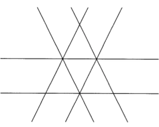
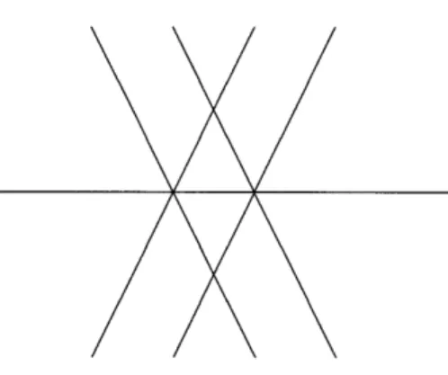
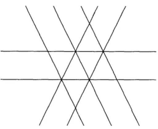
4.1 An arrangement of 4 lines in the plane . . . . 4.2 The intersection semilattice . . . . 6.1 The Shi arrangement of type A2 . . . . 6.2 The arrangement of type A2 for S = {12, 13} . . . .

6.3 Another deformation of A3. . . . ._. 6.4 The arrangement DO ...

6.5 The arrangementsB2 and C2 . . . .. . . . 6.6 The arrangements D2 and BC2 . . . .. . . . 6.7 The arrangement 3 . . . . . .. . . .

6.8 An alternating tree on 12 vertices . . . . 6.9 The arrangement ~A[,2] ...

7.1 The arrangement

A3

9.1 An example of a hypermatroid ... 9.2 Two hypergraphs ...

10.1 A hypergraph which is not normal . . . . 10.2 A hypergraph which is normal but does not satisfy (10.1) . . . .

15 22 46 46 64 66 71 73 77 78 81 82 85 90 13 19 128 .29

Part I

Chapter 1

Eigenvalues and counting

Spectral graph theory is a well developed area of mathematics which studies the eigenvalues of certain matrices associated to graphs. The motivation and applications of the theory lie very often within areas outside combinatorics, such as linear algebra, probability theory and geometry. The first part of the present thesis touches upon some combinatorial aspects of the theory. Classical expositions in spectral graph theory can be found in [21] and [29].

In the first part of this thesis we use an elementary enumerative method, that of counting closed walks, to obtain information about the adjacency eigenvalues associ-ated to special families of graphs. The spectral properties of such families of graphs seem to have puzzled mathematicians in recent years. When this counting method succeeds, it explains certain phenomena about eigenvalues of combinatorial matrices in a particularly elegant way. Traditionally, it has been used to obtain combinatorial information about a graph, given its adjacency eigenvalues. Here we proceed in the opposite direction.

Applied on different situations, this method often leads to various interesting combinatorial problems. These problems may or may not be easier to solve than the original problems which are usually stated in the language of linear algebra.

Overview of Part I. The rest of the introduction contains basic background from graph theory. We first give the necessary preliminaries about notation and terminology. Then we describe the basic enumerative method to compute eigenvalues and give a few examples. These include a proof of a classical theorem of linear algebra about the characteristic polynomials of AB and BA, where A and B are n x mrn and

rn x n matrices respectively.

In Chapter 2 we use the counting method to prove and generalize a conjecture of Propp, which was the motivation for the first part of this thesis. The basic result describes the adjacency eigenvalues of a directed graph D(G) associated to a given

directed graph G, in terms of the eigenvalues of the induced subgraphs and the Laplacian matrix of G. The vertices of the directed graph D(G) are the oriented rooted spanning trees of G and its edges are constructed using the so called re-rooting moves.

In Chapter 3 we consider another family of graphs which are conjectured to have remarkable spectral properties. These graphs were introduced in [31] by Hanlon and arose naturally from problems in Lie algebra homology. Our method reduces an important special case of Hanlon's conjecture, which remains open, to a purely combinatorial statement.

It would be interesting to find other graphs for which the method of counting closed walks gives nontrivial spectral information. Such an example appears in [18, Thm. 1] which implies that the even and odd "Aztec diamonds" ADn and ODn have identical nonzero eigenvalues.

1.1

Graphs and matrices

We think of a graph as a slightly more general object than a matrix with complex entries. We consider what is usually called a "weighted directed graph," to treat uniformly all kinds of graphs that will be of interest in this first part of the thesis.

The vertex set of a graph G is a finite, totally ordered set {v, v2, ... , vn}, denoted

V(G). For each ordered pair (vi, vy), there is a finite set of edges with initial vertex vi and terminal vertex v.. We denote such an edge by e = viv3 when this creates no ambiguity. We also say that e is directed from vi to vj. Each edge e has a nonzero complex number assigned to it, called the weight of e and denoted by wtG(e), or

simply by wt(e). We use the notation E(G) for the set of weighted edges of G. We write G = (V, E) to denote a graph with vertex set V and edge set E.

To each complex matrix A = (aij) we can assign a graph on the vertex set [n] =

{1,2,...,

whose (i,j) entry is the sum of the weights of all edges of G with initial vertex vi and terminal vertex vj. For many purposes, one can replace the edges directed from

vi to vy by a single edge with weight the sum of the weights of these edges, without

affecting definitions or results. The complication of multiple edges will be useful for technical reasons in Chapter 2, as well as in the proof of Theorem 1.4.1.

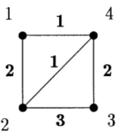
Ordinary, or else undirected graphs differ from the ones we have described in the fact that their edges have no orientation. That is, they have two endpoints which

1 4

2

1

2

2 3 3

Figure 1.1: An ordinary graph G

may coincide, with no distinction into initial and terminal vertex. However, we can consider ordinary graphs to be graphs as described above by replacing each edge e with a pair of edges with the same endpoints as e but of opposite orientation and weight the weight of e. Figure 1.1 shows an ordinary graph G on four vertices and the weights attached to the edges. Its adjacency matrix is the symmetric matrix

10 2 0

2031

11

2 0 3 1

A(G) _{0 3 0 2}

1 1 2 0

Walks and trees. Let 1 be a nonnegative integer. By an i-walk or an I-path W in a graph G = (V, E) we mean an alternating sequence (u0, e1, u•,..., el, ul) of vertices and edges of G such that for each 1 < i < 1, the edge ei has initial vertex

ui-1 and terminal vertex ui. We call I the length of W and the vertices u0 and ul its initial and terminal vertices, respectively. We call u0, ul,..., ul the vertices visited by

W. The walk is said to be closed if uo = ul. The weight of a walk is the product of the weights of its edges. More generally, by the weight of any object K associated to a graph, like a tree or a forest, we always mean the product of the weights of the edges of K. If K is a finite family of such objects, we usually refer to the sum of the weights of the objects in K as simply the "weighted number of objects" in KC. We sometimes refer to the cardinality of K as the "unweighted number of objects" in K, to emphasize the distinction.

If S is a nonempty subset of the vertex set V, we denote by Gs the induced subgraph of G on the vertex set S, that is the graph obtained from G by deleting the vertices not in S and all edges incident to them. The weights of the edges remaining are the same as in the original graph G. In the matrix language, this just means that we delete the rows and columns of A(G) which correspond to the vertices not in S. A subgraph is an induced subgraph with some of its edges deleted. It is called

spanning if its vertex set is V, the whole vertex set of G.

is a spanning subgraph T of G having a distinguished vertex r, called the root, such that for every v E V there is a unique path in T with initial vertex v and terminal

vertex r. A rooted forest on G with root set S is a spanning subgraph which is a union of vertex-disjoint rooted spanning trees on subgraphs of G. The roots of these trees are the elements of S. We call G strongly connected if for any two vertices u, v of G, there exists a walk in G with initial vertex u and terminal vertex v.

Homomorphisms. Now let G' = (V', E') be another graph. A graph homo-morphism

f

f

f

f

1.2

Laplacians and the Matrix-Tree theorem

Let G be a graph with n vertices and let u E V(G). The outdegree of u is the sum of the weights of the edges of G having initial vertex u, i.e. the sum of the entries in the row of A(G) corresponding to u. We denote by O(G) the diagonal n x n matrix with diagonal entries the vetrex outdegrees. The matrix L(G) = O(G) - A(G) is

called the Laplacian matrix of G. Note that it is independent of the loops of G, i.e. the edges whose initial and terminal vertices coincide. The Laplacian of the graph of Figure 1.1 is

/3

-2 0 -1

L(G)- -2 6 -3 -1

L(G)

0 -3 5 -2

I -1 -2 4

As it will be aparent from the theorem below, the Laplacian matrix gives valuable information about the graph. Its eigenvalues play an important role in spectral graph theory. For an exposition of many of the known results about Laplacians of ordinary graphs see [38].

The main result we will use about Laplacians is the following version of the Matrix-Tree theorem. A proof and a generalization can be found in [17]. Recall that by the weighted number of rooted forests below we mean the sum of their weights.

Theorem 1.2.1 For S C G we denote by L(G) s the submatrix of L(G) obtained by

deleting the rows and columns corresponding to the vertices in S. Then det(L(G) s) is the weighted number of rooted forests on G with root set S.

1.3

Eigenvalues and closed walks

Given a graph G, we call the eigenvalues of its adjacency matrix A(G) the adjacency

eigenvalues, or simply the eigenvalues of G. We denote by PG(A) the multiplicity of

A as an eigenvalue of G. We call the eigenvalues of L(G) the Laplacian eigenvalues

of G. We now relate the eigenvalues with the closed walks in G.

Let V(G) = {vi, v2,. .. ., vn . It is well known that the (i,j) entry of the matrix

A(G)' equals the weighted number of 1-walks in G with initial vertex vi and terminal vertex vj. Hence, the weighted number of closed 1-walks in G, which we denote by w(G, 1), equals the trace of A(G)1 and hence the sum of the 1th powers of the

eigenvalues of G.

Thus a common technique to count walks in G is to compute its eigenvalues. Our approach here will be the opposite. We will count the weighted number of closed walks in G combinatorially and then read off its eigenvalues from the answer. This will be possible thanks to the following elementary and well known fact.

Lemma 1.3.1 Suppose that for some nonzero complex numbers ai, bj, where 1 <

i < r and 1 < j < s, we have

r S

Ea.= b

(1.1)

i=1 j=1

for all positive integers 1. Then r = s and the ai are a permutation of the bj.

Proof: Multiplying (1.1) by xi and summing over 1 gives

r aix

bjx

1 - aix 1 - bx

i=1 j=1

for small x. Since clearing denominators we obtain a polynomial equation, this has to hold for all x. If -y is any nonzero complex number, we can multiply the equation above by 1 - -yx and set x = 1/7y to conclude that 7y appears among the ai as many times as among the b3. El

Example 1.3.2 To illustrate the idea, let r be a positive integer and consider the graph M,(r) on the vertex set [n] with r edges of weight 1 directed from vertex i to vertex j, for any i,j E [n]. Its adjacency matrix is easily seen to have nr as its only nonzero eigenvalue, its multiplicity being one. Alternatively, there are (nr)' ways to choose a closed l walk (uo, el, ul,..., el, ut) in M,(r). Indeed, we have ni choices for the vertices uo,..., u-1 and r choices for each edge ei. Hence

yielding the unique nonzero eigenvalue nr.

Example 1.3.3 Consider now the complete bipartite graph Hr,s, where r, s are positive integers. Its vertex set is the disjoint union of two sets [r] = {1,..., r} and [s]'= {1',..., s'} with r and s elements respectively. For each pair of vertices (a, b)

one of which is in [r] and the other in [s]', there is an edge with weight 1 directed from a to b.

It is not difficult to show directly that the nonzero eigenvalues of Hr,s are \s and - Vr-s, each with multiplicity one. To use the counting method instead, consider

a closed 1-walk (uo, el,u 1,...,el, uIl) in Hr,s. Clearly, no such walk exists if 1 is odd. There are 2(rs)' such walks if I is even, each with weight 1. Indeed, if uo E [r], there are r ways to choose each ui for even values of i and s ways to choose each u, for odd values of i, where 0 < i < I - 1 and similarly for the case uo E [s]'. Thus,

w(Hr,s

=

(

Vs)' +

)

and Lemma 1.3.1 gives the eigenvalues of Hr,s as promised.

1.4

Matrix products and eigenvalues

We now give a less trivial application of the counting method described in the previous section. The following theorem is a classical and useful result of linear algebra, rarely mentioned in introductory courses in the subject.

Theorem 1.4.1 If A and B are n x m and m x n matrices respectively having

complex entries, then the matrices AB and BA have the same nonzero eigenvalues, including multiplicities. In other words,

A' ch(BA, A) = A•m _{ch(AB, A), (1.2)}

where ch(T, A) = det(AI - T) is the characteristic polynomial of the square matrix T.

Simple linear algebra proofs appeared in [42][52][66] for the case where A and

B are square matrices. A proof of (1.2) for general A and B with entries from an

arbitrary commutative ring with a unit can be found in [51]. Of course, this more general statement follows immediately from the complex case. We believe that the combinatorial approach in the proof below provides a better understanding of this elementary fact.

Proof of Theorem 1.4.1: Consider a bipartite graph H on the vertex set [m] U [n]', where the notation is as in Example 1.3.3, with edges constructed as follows: For

each nonzero entry aij of A, include an edge directed from i' to

j

j'

Now construct two new graphs G1 and G2 on the vertex sets [m] and [n]'

respec-tively. The edges of G1 correspond to the walks of length 2 in H with initial (and

hence terminal) vertex in [m]. Specifically, for any two edges uv and vw in H with u, w

E [m], we construct an edge of G

and define its weight as the product of the weights in H of the edges uv and vw. Similarly, the edges of G2 correspond to the walks of length 2 in H with initial vertex

in [n]'.

It is easy to check that the adjacency matrices of the graphs G1 and G2 are the

martices BA and AB respectively. To prove the theorem, it is enough to prove that the sum of the weights of the closed walks of a given positive length 1 is the same for

G1 and G2. Hence, it suffices to establish a length and weight preserving bijection

between the closed walks of positive length of the two graphs. But, by construction, the closed walks of G1 are the closed walks (u1, v1, u2, v2,... , Uk, Vk, ul) of H with

Ul

E

E

(u1, V1, U22, V2,..., Uk, Vk, U1) - (V1, U2, V2,U3,...,Vk, U1, V1)

Chapter 2

Spectra of the Propp Graphs

2.1

The graph

D(G)

and Propp's conjecture

The graph D(G) was defined by Propp for "unweighted" directed graphs G, having no loops or multiple edges. We give here the definition more generally for an arbitrary graph G. This is possible since the concept of orientation for the edges is already inherent in our notion of a graph.

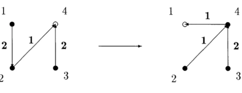
We first define what we mean by a re-rooting move on a graph G = (V, E). Let T

be a rooted spanning tree of G with root r. Let e E E be directed from r to u E V and denote by T(e) the tree obtained from T by adding the edge e and deleting the edge of T with initial vertex u. Note that T(e) is another rooted spanning tree of G with root u. We say that T(e) is obtained from T by a re-rooting move on G with respect to e. Figure 2.1 shows a re-rooting move on the graph of Figure 1-1 with respect to the edge directed from vertex 4 to vertex 1. The roots of the trees are drawn as unfilled circles and determine the orientation of the edges of the trees.

We can now give the definition of D(G).

Definition 2.1.1 (Propp) Let G = (V, E) be a graph. The new graph D(G) has as vertices the rooted spanning trees of G. Its edges are constructed as follows: Let T be a rooted spanning tree on G with root r. Let e be an edge in G with initial vertex r and weight wt(e) and let T(e) be the tree obtained from T by a re-rooting move on G with respect to e. Then add an edge in D(G) of weight wt(e), directed from T to T(e).

The idea of the construction of D(G) appeared for the first time implicitly in the proof of the Markov chain tree theorem by Anantharam and Tsoucas [2]. In this paper the authors needed to lift a random walk in a directed graph G to a random

2 4 1 2 1 4 2 2 3 2 3

Figure 2.1: A re-rooting move on G

walk in the set of arborescences of G, which coincides with the set of rooted spanning trees if G is strongly connected. On the other hand, Propp's motivation for defining

D(G) came from problems related to domino tilings of regions. The re-rooting move

on G is analogous to a certain operation on domino tilings, called an "elementary move" in [25]. In fact, under an appropriate coding, the elementary moves can be viewed as a special case of a type of move very similar to the re-rooting move. An even more general operation is described in [47]. Proposition 2.2.5, stated in §2.2, is the analogue of the fact that any domino tiling of a simply connected region can be obtained from any other tiling of the same region by a sequence of elementary moves. Thus D(G) encodes the ways one can reach any rooted spanning tree on G from any other, assuming that G is strongly connected, by performing re-rooting moves.

The main problem we pose here and answer in the following section is to describe the eigenvalues of D(G) in terms of information contained in the original graph G. The motivation for posing this question comes from a conjecture of Propp [46] con-cerning an interesting special case. We denote by H,, the complete graph on the vertex set [n] without loops. This means that for each pair (i,j) of vertices with

i 5 j, there is an edge in H,, with weight 1, directed from i to j. The Table 2.1 was

constructed by Propp. The entry in the row labeled with i and column labeled with

_j

Conjecture 2.1.2 (Propp) The Laplacian eigenvalues of D(H,) are all integers

ranging from 0 to n. The multiplicities of 0, 1, n - 1 and n are 1, n2 _{- 2n, 0 and}

nn - 1

- (n - 1)n-1 respectively.

In §2.3 we will prove Propp's conjecture and we will find the multiplicities of other eigenvalues.

0 1 2 3 4 5

2 1 1 2 2 2 2

3 1 4 4 9 9 9 4 1 9 27 27 64 64

5 1 16 96 256 256 625

Table 2.1: Sums of multiplicities of Laplacian eigenvalues of D(H")

2.2

Covering spaces of graphs and eigenvalues

We start with a few more useful definitions. Let G = (V, E) and C = (V, F) be two

graphs. We say that

G is a covering space of G if there exists a graph homomorphism

p : G -+ G with the following property: If p(t) = u and e E E is any edge in G with initial vertex u, then there is a unique edge E -k with initial vertex i such that

p(ý) = e. Such a homomorphism is called a covering map of graphs.

It follows immediately that given u, i as above and any walk W in G with initial vertex u, there is a unique walk W in

G

p-1(u) = {i E V I p(ii) = u} the fiber above u. Note that, by construction, the

Propp graph D(G) is a covering space of the graph G. Indeed, the covering map p maps each vertex T of D(G) to its root and each edge constructed by a re-rooting move on G with respect to e to the edge e in G. This observation will be fundamental in determining the eigenvalues of D(G).

To relate the weighted number of closed walks on G and 0, note that any closed walk in

G

or may not be closed. Let tp(W) be the number of it in the fiber p-1 (u) which yield

a closed walk in

G.

The following theorem gives an expression for w(G, 1) in a crucial special case. For any G and nonnegative integer 1, we will denote by g(G, 1) the sum of the weights of the closed 1-walks which visit all vertices of G.

Theorem 2.2.1 Let p : 0 -- + G be a covering map of graphs. Suppose that the

quantity t,(W) defined above, depends only on the set U of vertices visited by the closed walk W. We denote this quantity by tp(U). Then

w(C,1) = E rp(S) w(Gs, l), (2.1)

where

rn(S) = E (-

1

)#(U-S) t(U)

and V is the vertex set of G.

Proof: Let's fix a subset U of the vertex set V of G. Let W be a closed 1-walk

in G such that U is the set of vertices visited by W. As we have remarked before, any closed i-walk in G projects under p to such a walk W, for some U C V. The unweighted number of closed walks in G which project to W is, by assumption, tp(U). Since p is weight preserving, it follows that

w(G, 1) = E t

(U) g(Gu, 1).

(2.2)

UCV The inclusion-exclusion principle gives

g(Gu,1) = 1 (- 1)#(U-s) w(Gs,1). (2.3)

SCU

Hence, after using (2.3) to compute g(Gu,1) and changing the order of sumation, (2.2) becomes

w(G, 1)

=

E

w(Gs, 1)

E

(-~1)#(U-S)t(U),

SCV SCUCV

which is equivalent to (2.1). El

From Theorem 2.2.1 and the discussion in §1.3 we get immediately the following corollary.

Corollary 2.2.2 Under the assumptions of Theorem 2.2.1, the nonzero eigenvalues

of G are included in the nonzero eigenvalues of the induced subgraphs of G. Moreover, if 7 0 then the multiplicity of 7y as an eigenvalue of G is

E rp(S) P G ),

SCV

where bGs(7) _{stands for the multiplicity of- as an eigenvalue of Gs. El}

Corollary 2.2.3 Under the assumptions of Theorem 2.2.1, for all complex numbers 7 0 we have

rS(S) PGs(') > 0.

SCV

We now specialize the above results to describe the eigenvalues of the Propp graphs and their multiplicities.

Corollary 2.2.4 For a graph G on the vertex set V we have w(D(G),l) = E det(L(Go) s - I) w(Gs,1),

SCV

where Go is the graph obtained from G by replacing all weights of its edges with 1 and I denotes the identity matrix of the appropriate size. The nonzero eigenvalues of D(G) are included in the nonzero eigenvalues of the induced subgraphs of G. Moreover, if₇ =0 then the multiplicity of 7 as an eigenvalue of D(G) is

S

SCV

In particular, for all complex numbers / 5 0 we have

Sdet(L(Go)Is

Proof: Let p : D(G) -+ G be the covering map defining D(G). We will show

that it satisfies the assumption of Theorem 2.2.1 and that rp(S) = det(L(Go) Is - I).

The assertions follow from Theorem 2.2.1 and its corollaries.

Let W = (uo, elI,u,...,e1,ul) be a closed 1-walk in G with initial vertex u0 = r.

Let U be the set of vertices visited by W. Consider the lift W = (To, 61, T₁,..., ,, T,) of W in D(G) with initial vertex the spanning tree T = To on G, rooted at r. We

want to compute the unweighted number tp(W) of all such T for which the walk W

satisfies T1 = T.

At each step of the walk W from Ti- 1 to Ti we add the edge ei, which is directed from ui-1 to ui and delete the edge with initial vertex ui. Therefore, at the end of our walk TI, a vertex of G appearing for the last time in W as ui-1, where 2 < i < 1, will be directed to ui with ei and the vertices of G not visited by W will be directed as in

To. To construct a rooted tree T = To with the desired property, we have to choose an

edge with initial vertex u for any vertex of G other than r. The edges are prescribed by W for the vertices in U and we are free to choose the rest to produce a spanning tree, rooted at r. It follows that tp(W) is the number T(Go, U) of rooted forests on Go with root set U. This indeed depends only on U. The expression det(L(Go)s - I) for the alternating sum

rp(S) = (-1)#(U-s) T(Go, U)

SCUCV

follows from the Matrix-Tree theorem (Theorem 1.2.1) and some elementary linear algebra. D

Zero as a Laplacian eigenvalue. At this point we digress to show directly that zero is a simple eigenvalue of the Laplacian of D(HI), meaning that its multiplicity

is 1. In the remaining of this section we assume that all edges of G have weight 1. Suppose that G is a disjoint union of strongly connected graphs. Then the multiplicity of 0 as an eigenvalue of the Laplacian of G is the number of connected components of G. Indeed, a basis of the corresponding eigenspace is the set of vectors with entry 1 on the vertices of G belonging to a given connected component and 0 on the rest. Hence in particular, if D(G) is strongly connected then L(D(G)) has zero as a simple eigenvalue. In general, D(G) might be disconnected even though G is connected. The same is not true, however, with strong connectedness. The following proposition, proved independently for the first time by Propp, shows that D(H,) is indeed strongly connected.

Proposition 2.2.5 If G = (V, E) is strongly connected then so is D(G). In

partic-ular, the Laplacian of D(G) has zero as a simple eigenvalue.

Proof: Given two oriented spanning trees To and T1 on G with roots ro and rl, we want to find a walk in D(G) from To to T1. Such a walk is the lift of the walk in G directed from r0 to ri, constructed as follows: We start at ro and follow the unique

path in T1 from r0 to rl. Then we pick the furthest vertex v in G away from r, and follow the shortest walk in G (with respect to length) from r, to v. This can be done by strong connectedness of G. Now we follow the unique path in T1 from v to r, and continue in the same way with the second furthest vertex in G away from r, until only r, remains. At this point we stop.

This walk has the property that the last time a vertex u other than r, is visited by our walk, it is followed by its successor in T1, and hence it induces a walk in D(G) from To to T1. E

2.3

Applications and the proof of Propp's

conjec-ture

Recall that the complete graph H, is the graph on the vertex set [n]= {1,2,... ,n} with exactly one edge of weight 1 directed from i to j for each i

j

E

Proposition 2.3.1 The adjacency eigenvalues of D(H,), where n > 2, are -1, 1,

., n. - 1. The multiplicity of i is

(

i+ )1 (n

- )

< n

nn- 1

- (n - 1)n - 1

Proof: The induced subgraphs of H, are isomorphic to Hm for some 1 < m < n.

It is easy to show directly that the eigenvalues of Hm are m - 1 with multiplicity 1 and -1 with multiplicity m - 1. Hence, by Corollary 2.2.4, the nonzero eigenvalues of D(H,) are included in the set {-1, 1,..., n - 1}. Moreover the eigenvalue m - 1, for 2 < m < n, has multiplicity

(n) det(L(Hn)[m] - I) = ( ( m - 1)(n - 1)n-m - 1

m m

while -1 has multiplicity

S

(m - 1) det(L(Hn)[m] - I)

n

=

Z(m

n

m=1 m

We have evaluated the last sum by classical elementary methods. The multiplicities we have so far add up to nn- 1_{, so 0 is not an eigenvalue of D(HI) and the proposition} follows. n

Corollary 2.3.2 The Laplacian eigenvalues of D(Hn), wheren > 2, are 0, 1,... n-2, n. The multiplicity of i is

(n-i-1) (n) -1) - 1 if 0<i<n-1;

nn - 1 _{- (n - 1)-1}

_{if i}

L(D(Hn)) = (n - 1)I - A(D(Hn)).

As a variation of the above result we give the following proposition. Its proof consists of a similar computation and is omitted.

Proposition 2.3.3 Let M,(r) be the graph on the vertex set [n] of Example 1.3.2,

having r edges of weight 1 directed from i to

j,

ID(Mn(r))(r) =f(ir - 1)

()

(nrr)n -1 _{- (nr - 1)}n

-1 if i = 0.

As a final specialization of Corollary 2.3, we consider the complete bipartite graph

H,,s of Example 1.3.3.

Proposition 2.3.4 The nonzero eigenvalues of D(H,,s) are pq and -p/q for

1 < p < r, 1 < q < s. The characteristic polynomial of its adjacency matrix is

r 8

x t

] fi

p=l q=1

where t is a nonnegative integer depending on r, s and

m(p, q) = (r) - 1)r-- (s - 1)-p-l ps-pq-r-s+

p q

Note that m(p,q) is to be interpreted as 1 if r = p = 1, q = s, 0 if r = p = 1, q < s and similarly for the case s = q = 1.

Proof: There are ()

(s)

0 < q < s. The ones with p = 0 or q = 0 have only zero eigenvalues. We proved in Example 1.3.3 that the nonzero eigenvalues of Hp,q, where p and q are positive, are vpq and -vpq, each with multiplicity one. Therefore Corollary 2.2.4 gives the set of eigenvalues proposed as the nonzero eigenvalues of D(Hr,s). Morover, the multiplicity of Vq and -Vpq contributed by the Hp,q induced subgraphs is

m(p, q) = (r) (s) det(L(Hr,,s)|[p]u[q]I - 4

The above determinant equals

det(C D

where

A

can easily be shown to equal

(r - 1)s-q- (s - 1)r-P-l(qr

+

+

using elementary row and column operations. This yields the suggested value of

m(p, q) and completes the proof of the proposition.

L-Some further questions. The method of counting closed walks was successful in determining the adjacency eigenvalues of the Propp graphs D(G). It does not seem to be strong enough to give other information about these matrices, such as their

eigenvectors or the structure of their Jordan canonical forms. Since these matrices are not necessarily symmetric, in general they are not diagonalizable and hence they have nontrivial Jordan canonical forms. We would thus like to pose the problem of describing the eigenspaces of these matrices, as it was possible to do for the 0-eigenspace of a Laplacian, and their Jordan canonical forms, in terms of information about the original graph G. We have no indication that these questions have elegant answers.

The Jordan block structure of the Propp matrices L(D(H,)) has been computed for n = 2, 3,4 by A. Edelman [23]. For n = 3 the eigenvalue 3 has one 1 x 1 and two 2 x 2 Jordan blocks and for n = 4 the eigenvalue 4 has four 1 x 1, twelve 2 x 2 and three 3 x 3 Jordan blocks. The rest of the eigenvalues for these values of n were found to be semisimple.

Chapter 3

The Hanlon Graphs

In this chapter we are concerned with another interesting family of graphs, defined by Hanlon in [31]. These graphs, which we call the Hanlon graphs, arose in the study of the Laplacian operator on certain complexes associated to the Heisenberg Lie algebra. We consider the Hanlon graphs here because they are conjectured in [31, §1] to have very interesting spectral properties. Unlike the situation with the Propp graphs, Hanlon's eigenvalue conjectures remains largely untouched.

In this chapter we apply the method of counting closed walks to reduce an im-portant special case of Hanlon's conjecture to a purely combinatorial statement. We believe that our arguments, although incomplete, help to some extent to understand why the Hanlon conjectures might be true.

3.1

Hanlon's eigenvalue conjecture

We begin with the relevant notation and background from [31].

The Heisenberg and related Lie algebras. Let N be the 3-dimensional Heisenberg Lie algebra. As a complex vector space, N has a basis {e, f, x} with Lie

brackets

[e,f] = z, [e, x] = [f, x] = 0. Now fix a nonnegative integer k and let Nk be the Lie algebra

_H = - ® (C[t]

/

where (tk+ l) is the principal ideal in C[t] generated by tk+1. The Lie bracket in Wk is given by

For i E [0, k] = {0, 1,... , k}, let ei,

fi

them having the form

[ei, fi] = xi+3,

where i +

j

fi

Wk= E FeF X and also

A'k = (AE) A (AF) A (AX),

where A stands for the exterior algebra. For a set of indices I = {il, i2, ... ,•r

with 0 _ i < i2 < <

4

eI = e, A e2 A... A eir, and similarly for

ft

eA _A fB A xc,

where A, B and C range over all subsets of [0, k], form a basis of A-k, which we call the standard basis. Denote by Vk(a, b, c) the subspace (AtE) A (AbF) A (AcX) of Ak-.

Its standard basis consists of the elements eAA fB A xc satisfying #A = a, #B = b

and #C = c.

Lie algebra homology and the Laplacian operator. Let

a:

a

defined on elements of the standard basis by

8(m1 A n2 A . .. A,) 1) i+3j-1 [ni, rml 7•1 A ... A mi A .. A mj A . A rnr l<_i<j<_r

where m {e, f,x}. Then

a

=

0

H*(7-k) = ker / Im 0

is the (Lie algebra) homology of k7-. Define the Laplacian operator L : A-k - A'-k

to be

L

=

aa*

+

a*a,

where the adjoint of 0 (the coboundary map) is taken with respect to the Hermitian form for which the standard basis of Al-k is orthonormal. This operator is not to be confused with the Laplacian matrix of a graph. It is proved in [36] that ker L and H.(-Wk; C) are isomorphic as graded vector spaces, so that the (graded) multiplicity of zero as an eigenvalue of L gives the dimensions of homology groups of 7-Wk. The grading on Al-k is obtained by assigning degree 1 to each nonzero element of -Wk, so

that nonzero elements of Vk(a, b, c) have degree a + b + c. The maps 0 and a* do not preserve this grading since

a: Vk(a,b,c) - Vk(a - 1, b - 1,c + 1)

and

*: Vk(a - 1, b - 1, c + 1) ---+ Vk(a, b, c),

although L does. Each subspace Vk(a, b, c) is therefore invariant under L. It is also clear that a and &* do preserve another grading of A7-k, defined by assigning degree

i to ei,

fi

degree |

A|| +

IB||

+

IICI|,

|IS||

The matrix representing the restriction of the Laplacian L to Vk(a, b, c) with re-spect to the standard basis is the main object of study in [31]. This matrix is sym-metric, since the Laplacian is a self-adjoint operator. The graph which corresponds to this matrix (see §1.1) is denoted in [31] by Gk(a, b, c). The component Gk(a, b, c; w) of Gk(a, b, c) corresponds to the matrix representing the restriction of L to the ho-mogeneous component of Vk(a, b, c) of total weight w. Thus Gk(a, b, c) is the disjoint union of the graphs Gk(a, b, c; w), for all possible values of w.

In [31], Hanlon is primarily concerned with the families of graphs Gk(a, b, 0) and

Gk(a, b, 0; w), which are denoted by Gk(a, b) and Gk(a, b; w) respectively, for

simplic-ity. Let 1k (a, b; r) be the multiplicity of r as an eigenvalue of Gk(a, b). Let also

Mk(x, y, A) =J [k(a, b; r) Xayb Ar

a,b,r

be the generating function for these multiplicities. Hanlon's remarkable conjecture can be stated as follows. We refer the interested reader to [31] for more information. Conjecture 3.1.1 (Hanlon [31]) The eigenvalues of Gk(a, b) are all nonnegative

integers. Moreover,

k

Mk(x,y,A) -

fl(1

i=O

Hanlon determined explicitly the eigenvalues of Gk(a, b; w) under certain restric-tions on the parameters, the so called stable case [31, Thm. 2.5]. Since for most values of a, b and k, some values of w are not stable, the above conjecture remained unsettled for almost all cases. The note [1] contains a proof of Hanlon's conjecture in the following cases:

(ii) a = 1, arbitrary b and k (the zero eigenvalue).

A conjecture for more general nilpotent Lie algebras is stated in [31, §3]. In the next section we describe a slightly more general version of Conjecture 3.1.1 and its interpretation in terms of closed walks in a graph.

3.2

Closed walks in the Hanlon graphs

The graphs Gk(a, b; w) are described in [31, §1]. We will consider here only the graphs

Gk(a, b) which are the relevant to Conjecture 3.1.1. This conjecture implies that their

connected components Gk(a, b; w) also have nonnegative integers as eigenvalues. Combinatorial description of the Hanlon graphs. Note that

a*

Vk(a, b, 0). Hence the restriction of the Laplacian L on Vk(a, b, 0) has the form

a*a,

where

a:

and

* : Vk(a- 1, b - 1,1) --+ Vk(a, b, 0).

The vertex set of Gk(a, b) consists of all pairs (A, B) of subsets of [0, k], satisfying

#A

(U, V) and (X, Y) be vertices of Gk(a, b). There is an edge between these two vertices

if there exist u E U, v E V and z E Z such that

(i) X = (U - {u}) U {u + z}, (ii) Y = (V - {v})U {v - z}, (iii) u +v < k.

Clearly, this relation is symmetric in (U, V) and (X, Y). Let U = {ul, u2,..., Ua}<

and V = {v1i, v2,..., Vb}< and suppose that u = u, and v = v-. To each triple (u, v, z), as above, corresponds naturally the sign C162, where

eu, A ... A eui+z A ... A eua = 61 ex

and

ev, A ... A e,-z A ... A e b =6 2 ey

in the exterior algebra. The weight of the edge between (U, V) and (X, Y) is the sum of the signs corresponding to all such triples (u, v, z). If (U, V) 4 (X, Y) there is at

most one such triple and the weight of a possible edge is +1. On the other hand we have z = 0, C1 = 62 = 1 if X = U, Y = V and hence there is a loop of weight at most ab attached to some of the vertices of Gk(a, b).

For example, the component G2(2, 2; 4) of the graph G2(2, 2) has vertices (01, 12), (02,02) and (12, 01). Its adjacency matrix is

311

1 3 1 1 1 3

and its eigenvalues are 2, 2 and 5.

A generalization. We consider here a generalization of the graphs Gk(a, b) and of Conjecture 3.1.1, due to Hanlon. Let's fix two variables 7, 0. We can assume that they are complex variables. The new graphs depend also on the additional parameters

a, b, k. We denote them by Fk(a, b), supressing the dependence on r, 0. The vertex

set of Pk(a, b) is the same as that of Gk(a, b), i.e. the set of pairs (A, B) of subsets of [0, k], satisfying #A = a and #B = b. There is an edge in k (a, b) between (U, V) and (X, Y) if there exist u E U, v G V, I E X, J E Y with

I+J-u+v (mod k

+

(i) X = (U- {u})U {I},

(ii) Y = (V

-

{v}) U {J}.

The weight corresponding to such a quadruple (u, v, I, J) is the sign 1 (₂, calculated as before, possibly muliplied by q or 0 or both. The sign is multiplied by J if u + v > k and by 0 if I + J > k. The weight of the edge between (U, V) and (X, Y) is the sum of the weights corresponding to all such (u, v, I, J).

As an example, consider the component F3(2,3; 6) of F3(2, 3), with vertices of

weight 6. These vertices are (01,023), (02,013), (03,012) and (12,012). The adja-cency matrix of F3(2, 3; 6), with the given ordering of the vertices, is

5 + 70 1 -790 1

1

5 + 0

7790

1

-r70

r0

_{+ 2T0}

₀

Note that Fk(a, b) reduces to Gk(a, b) if T = 0 = 0. Let Uk(a, b; r) be the multi-plicity of r as an eigenvalue of Fk(a, b) and also

Nk(x, y,

A,

p)

=

b;

n +

m0)

xaybA

a,b,n,m

The generalization of Hanlon's eigenvalue conjecture is as follows.

Conjecture 3.2.1 (Hanlon) The eigenvalues of Fk(a, b) are all of the form n+mrO, where n, m are nonnegative integers. Moreover,

k

Nk(x,y, A,p)=l(1 + x + y + A k+1-ipi xy). (3.1) i=0

Closed walks. We now consider the counting method of §1.3. The weighted number of closed 1-walks in Fk(a, b) has a purely combinatorial description. Thus, it is a combinatorial challenge to show that w(Fk(a, b), 1) equals the sum of the 1 powers of the eigenvalues n + mr0 with the multiplicities predicted by (3.1). To state this more precisely, let

ti

Fa,b,k(t) =

w(Fk(a, b),

1)

1>0

be the exponential generating function of the weighted number of closed 1-walks in lk(a,

b). Since w(Fk(a, b), 1) is the sum of the

powers of the eigenvalues of

Fk(a,

b),

Fa,b,k(t) is a sum of exponentials of the form e0, where 7y is such an eigenvalue.

Conjecture 3.2.1 translates into the equation

k k

SFa,b,k(t)

(

a,b=O0 i=0

where we have set p = A7e. The weights of the closed walks in Fk(a, b) carry a sign. The general idea to approach (3.2) is to use an involution principle argument to cancel most of these weights and enumerate easily the rest. Let Fk be the disjoint union of the graphs Fk(a, b) for all a,b E [0, k]. The first part of Conjecture 3.2.1

would follow from the specialization x = y = 1 of (3.2):

tI k

w(Fkl) = I(3 + et(k+1-i+iO)).

_(3.3)

I>0 i --0

Let us describe first in detail the closed 1-walks in Fk(a, b). It is easier to do this with an example. The following is a closed 4-walk in P3(2, 3):

If an edge has initial vertex (U, V), the ^ sign is used to indicate the element of U or V which is subject to change and not a missing element. We think of the vertices of these walks as pairs of sequences of length a and b respectively. Each sequence has nonrepeated elements and the ones in the initial vertex are strictly increasing. The weight of the walk (3.4) has sign -1 since the signs of the permutation maps 02 - 20 and 013 -- + 301 are -1 and +1 respectively. The total weight of the walk is -(,q0)2 since the four edges are weighted, except for sign, by r]0, 0, iJ and 1

respectively. As an immediate product of the counting method we get the following proposition.

Proposition 3.2.2 Given k,a,b, the eigenvalues of Fk(a,b) depend only on the product 9O.

Proof: In view of the discussion in §1.3, it suffices to show that any closed walk W in Fk(a, b) has weight of the form +(r,0)s, for some nonnegative integer s. Consider

the sum of the elements of A and B, where (A, B) is a vertex of W. An edge with weight ±1 or +r10 leaves this sum unchanged when we move from the initial to the terminal vertex. An edge with weight +ir decreases the sum by k + 1, while an edge with weight ±0 increases the sum by k + 1. Since the walk is closed, there are as many edges with weight ±T1 as edges with weight +0. E

Nonreduced walks. We now consider a variation of the closed walks in Fk(a, b). A nonreduced 1-walk in Fk(a, b) is an 1-walk in Fk(a, b) except that we allow multiple

elements in the sets A, B of vertices (A, B) other than the initial vertex. A nonreduced walk is closed if its initial and terminal vertices coincide, except for the order within each coordinate. An example of a nonreduced closed 4-walk in P3(2, 3) is

(02, 013)

--

+ (il, 1i3) -- + (21, 13) -+ (2,

1131)

-+ (20,031).

(3.5)

Nonreduced walks are somewhat simpler to work with, since we don't have to guarantee nonrepeated elements at each step. Let w(Fk(a, b), 1) be the sum of the

weights of all nonreduced closed 1-walks in Pk(a, b). For our purposes, we can replace closed walks in Fk(a, b) with nonreduced closed walks, as the next proposition shows. We refer to U and V as the first and second coordinate respectively of a vertex (U, V). Proposition 3.2.3 For each I > 0 we have