Approaches to modeling market liquidity

(1)

Approaches to Modeling Market Liquidity

by

Annie Shoup

B.S., Massachusetts Institute of Technology (2016)

Submitted to the Department of Electrical Engineering and Computer

Science

in partial fulfillment of the requirements for the degree of

Master of Engineering in Electrical Engineering and Computer Science

at the

MASSACHUSETTS INSTITUTE OF TECHNOLOGY

June 2019

c

Massachusetts Institute of Technology 2019. All rights reserved.

Author . . . .

Department of Electrical Engineering and Computer Science

May 24, 2019

Certified by . . . .

Dr. Peter Kempthorne

Department of Mathematics

Thesis Supervisor

Accepted by . . . .

Katrina LaCurts

Chair, Master of Engineering Thesis Committee

(2)

(3)

Approaches to Modeling Market Liquidity

by

Annie Shoup

Submitted to the Department of Electrical Engineering and Computer Science on May 24, 2019, in partial fulfillment of the

requirements for the degree of

Master of Engineering in Electrical Engineering and Computer Science

Abstract

Intraday data was collected for the U.S. Financial Sector ETF and two of its com-ponent stocks: Bank of America and Citigroup. The analysis period includes 32 trading days, ranging from February 4, 2019 to March 20, 2019. From this trade and quote data, we construct 2,496 five-minute aggregate time bars for each security and calculate a series of spread, volume, depth, trade count, and price change liquidity measures. We examine the summary statistics of these liquidity measures before ap-plying principal components analysis to them through which we identify key liquidity dimensions in each security and common liquidity dimensions across them. Vector autoregressive models are applied to these principal component scores in order to gain further insight into their time series structure and the ways in which the measures interact over a 32-day period. Finally, the same methodology of principal components and time series analyses are applied to daily-normalized liquidity measures in order to better understand the intraday, rather than multi-day, dynamics of liquidity. Thesis Supervisor: Dr. Peter Kempthorne

(4)

(5)

Acknowledgments

Dr. Kempthorne, thank you for your continued support and guidance throughout this process. This thesis was a truly invaluable experience from which I learned an incredible amount.

Samira and Andrew, thank you for always providing me a comfortable couch to work from.

Emma, thank you for providing me with multiple comfortable couches to work from; the leather sectional in your living room is entirely responsible for Chapter 2 of this thesis.

Allison, Alex, Isabella, and Lexi, while you didn’t provide me any couches to work from (hence being mentioned fourth), thank you for the constant encouragement and optimism that you did provide me with throughout this process.

Finally, thank you to Ben (and Pilgrim). I would not have been able to finish this without you.

(6)

(7)

List of Figures

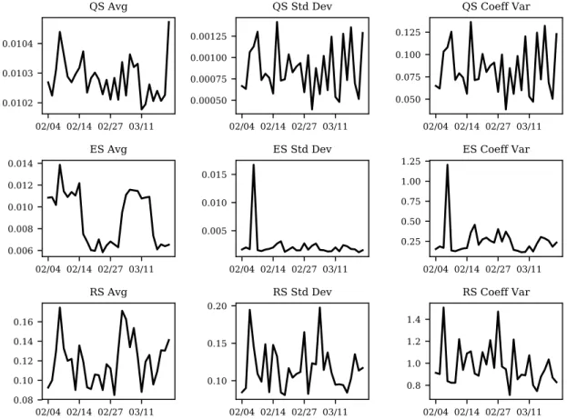
4-1 The average, standard deviation, and coefficient of variation of Bank

of America’s spread measures, aggregated across 2,483 five-minute bars. 56

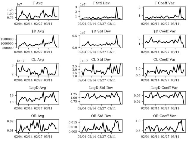
4-2 The average, standard deviation, and coefficient of variation of Bank

of America’s volume and depth measures, aggregated across 2,483

five-minute bars. . . 58

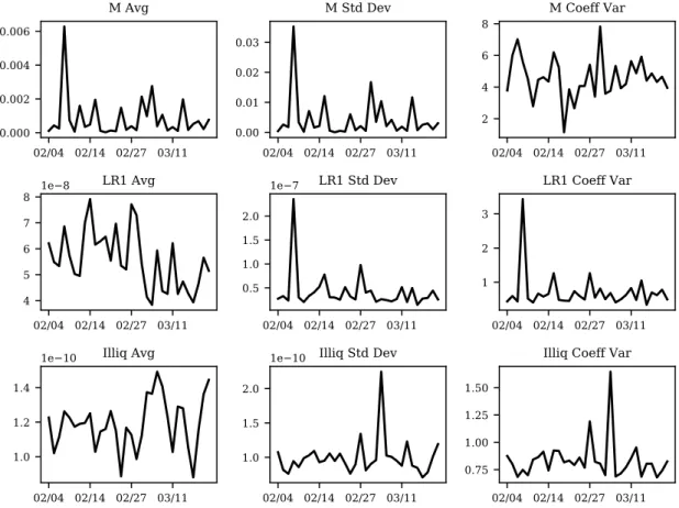
4-3 The average, standard deviation, and coefficient of variation of Bank of

America’s trade count measures, aggregated across 2,483 five-minute

bars. . . 60

4-4 The average, standard deviation, and coefficient of variation of Bank of

America’s price-change measures, aggregated across 2,483 five-minute

bars. . . 61

4-5 The Z-scores of Bank of America’s liquidity measures averaged across

15-minute intervals. . . 62

4-6 The average, standard deviation, and coefficient of variation of

Citi-group’s spread measures, aggregated across 2,485 five-minute bars. . . 64

Cit-igroup’s volume and depth measures, aggregated across 2,485

Citi-group’s trade count measures, aggregated across 2,485 five-minute bars. 69

(12)

4-10 The Z-scores of Citigroup’s liquidity measures averaged across

4-11 The Z-scores of Citigroup’s spread measures averaged across 15-minute

intervals. . . 73

4-12 The Z-scores of Citigroup’s volume and depth measures averaged across

4-13 The Z-scores of Citigroup’s trade count measures averaged across

4-14 The Z-scores of Citigroup’s price change composite measures averaged

across 15-minute intervals. . . 76

4-15 The average, standard deviation, and coefficient of variation of the Financial Sector ETF’s spread measures, aggregated across 2,496

4-16 The average, standard deviation, and coefficient of variation of the Financial Sector ETF’s volume and depth measures, aggregated across

2,496 five-minute bars. . . 80

4-17 The average, standard deviation, and coefficient of variation of the Financial Sector ETF’s trade count measures, aggregated across 2,496

4-18 The average, standard deviation, and coefficient of variation of the Financial Sector ETF’s price-change measures, aggregated across 2,496

4-19 The Z-scores of the Financial Sector ETF’s liquidity measures averaged

4-20 The Z-scores of the Financial Sector ETF’s spread measures averaged

4-21 The Z-scores of the Financial Sector ETF’s volume and depth measures

averaged across 15-minute intervals. . . 87

4-22 The Z-scores of the Financial Sector ETF’s trade count measures

(13)

4-23 The Z-scores of the Financial Sector ETF’s price change composite

measures averaged across 15-minute intervals. . . 89

5-1 The scree plot of Bank of America’s principal components resulting

from PCA on 13 liquidity measures. . . 96

5-2 The principal component loadings of Bank of America resulting from

PCA on 13 liquidity measures. . . 97

5-3 The scree plot of Citigroup’s principal components resulting from PCA

on 13 liquidity measures. . . 102

5-4 The principal component loadings of Citigroup resulting from PCA on

13 liquidity measures. . . 102

5-5 The scree plot of the Financial Sector ETF’s principal components

resulting from PCA on 13 liquidity measures. . . 107

5-6 The principal component loadings of the Financial Sector ETF

result-ing from PCA on 13 liquidity measures. . . 108

6-1 The cumulative sum of Bank of America’s principal components scores

over time. . . 115

6-2 The autocorrelation and cross-correlation of Bank of America’s

princi-pal component scores. . . 117

6-3 The autocorrelation and partial autocorrelation of Bank of America’s

first principal component’s scores. . . 118

second principal component’s scores. . . 119

third principal component’s scores. . . 120

fourth principal component’s scores. . . 121

(14)

6-8 The partial autocorrelation of Bank of America’s principal component

scores. . . 123

6-9 The cumulative sum of Citigroup’s principal components scores over

time. . . 129

6-10 The autocorrelation and cross-correlation of Citigroup’s principal

com-ponents scores over time. . . 131

6-11 The partial autocorrelation and partial cross-correlation of Citigroup’s

principal components scores over time. . . 132

6-12 The cumulative sum of the Financial Sector ETF’s significant principal

components’ scores over time. . . 137

6-13 The autocorrelation and cross-correlation of the Financial Sector ETF’s

principal components scores over time. . . 139

6-14 The partial autocorrelation and partial cross-correlation of the

Finan-cial Sector ETF’s principal components scores over time. . . 140

7-1 The scree plot of Bank of America’s principal components resulting

from two principal component analyses; one on daily-normalized mea-sures and the other on meamea-sures normalized over a 32-day time period. 147

7-2 Bank of America’s principal component loadings from principal

com-ponents analysis on 13 daily-normalized liquidity measures. . . 148

7-3 The scree plot of Citigroup’s principal components resulting from two

principal component analyses on 13 liquidity measures normalized daily

and normalized over the entire 32-day time period. . . 152

7-4 The principal component loadings of Citigroup resulting from PCA on

13 liquidity measures. . . 153

7-5 The scree plots of the Financial Sector ETF’s principal components

resulting from two principal component analyses, one on 2,946 obser-vations of 13 liquidity measures each, where one analysis normalizes the measures over the entire time period (32 days) and the other

(15)

7-6 The principal component loadings of the Financial Sector ETF result-ing from PCA on 2,496 daily-normalized observations of 13 liquidity

measures. . . 159

8-1 The cumulative sum of BAC’s principal components scores over time. 165

8-2 The autocorrelation and cross-correlation of Bank of America’s

princi-pal components scores of Daily-normalized Liquidity measures. . . 166

8-3 The partial autocorrelation of Bank of America’s principal components

scores of daily-normalized liquidity measures. . . 167

8-4 The cumulative sum of Citigroup’s principal components scores over

time. . . 171

8-5 The first principal component’s results from a second-order VAR model

applied to Bank of America’s principal component scores. * indicates t value is less than 0.001. ** indicates t value is less than 0.01. ***

indicates t value is less than 0.05. . . 171

8-6 The autocorrelation and cross-correlation of Citigroup’s principal

com-ponents scores of daily-normalized liquidity measures. . . 173

8-7 The partial autocorrelation of Citigroup’s principal components scores

of daily-normalized liquidity measures. . . 174

8-8 The cumulative sum of the Financial Sector ETF’s principal

compo-nents scores over time. . . 177

8-9 The autocorrelation and cross-correlation of the Financial Sector ETF’s

principal components scores of daily-normalized liquidity measures. . 178

8-10 The partial autocorrelation of the Financial Sector ETF’s principal

(16)

(17)

List of Tables

2.1 A brief summary of the spread measures discussed where p is the asset

price, a is the ask side, b is the bid side, m is the mid, t indicates an executed trade, and n is an amount of time over which price impact is

measured. . . 36

3.1 The largest constituents that make up the Financial Select Sector

SPDR Fund as of March 22, 2019. Only Bank of America and

Cit-igroup are included in this analysis. . . 46

3.2 The top 10 holdings by market value of XLF as of March 22, 2019. . 46

4.1 Summary statistics of Bank of America’s spread measures; these

en-compass 2,483 five-minute bar observations for each measure. . . 54

4.2 Summary statistics of Bank of America’s volume and depth measures;

these encompass 2,483 five-minute bar observations for each measure. 57

4.3 Summary statistics of Bank of America’s trade count measures; these

encompass 2,483 five-minute bar observations for each measure. . . . 59

4.4 Summary statistics of Bank of America’s liquidity measures involving

price changes; these encompass 2,483 five-minute bar observations for

each measure. . . 60

4.5 Summary statistics of Citigroup’s spread measures; these encompass

2,485 five-minute bar observations for each measure. . . 65

4.6 Summary statistics of Citigroup’s volume and depth measures; these

(18)

4.7 Summary statistics of Citigroup’s trade count measures; these

encom-pass 2,485 five-minute bar observations for each measure. . . 68

4.8 Summary statistics of Citigroup’s liquidity measures involving price

changes; these encompass 2,485 five-minute bar observations for each

measure. . . 69

4.9 Summary statistics of the Financial Sector ETF’s spread measures;

these encompass 2,496 five-minute bar observations for each measure. 77

4.10 Summary statistics of the Financial Sector ETF’s volume and depth measures; these encompass 2,496 five-minute bar observations for each

measure. . . 79

4.11 Summary statistics of the Financial Sector ETF’s trade count mea-sures; these encompass 2,496 five-minute bar observations for each

measure. . . 81

4.12 Summary statistics of the Financial Sector ETF’s liquidity measures involving price changes; these encompass 2,496 five-minute bar

obser-vations for each measure. . . 83

5.1 The principal components of Bank of America using PCA on 13

liq-uidity measures and the Kaiser criterion to determine significance. . . 96

5.2 The principal component loadings of each of Bank of America’s 13

liquidity measures across components. . . 97

5.3 A varimax rotation of Bank of America’s first five principal component

loadings resulting from principal components analysis on liquidity

mea-sures. . . 99

5.4 Percentage of cumulative variance of each of Bank of America’s original

liquidity measures as explained by the five significant PCA components.101

5.5 The principal components of Citigroup using PCA on 13 liquidity

mea-sures and the Kaiser criterion to determine significance. . . 101

5.6 The principal component loadings of Citigroup using PCA on 13

(19)

5.7 A varimax rotation of Citigroup’s first four principal component load-ings resulting from principal components analysis on liquidity measures.104

5.8 The variance of Citigroup’s original variables explained by the

signifi-cant principal components. . . 105

5.9 The principal components of the Financial Sector ETF using PCA on

13 liquidity measures and the Kaiser criterion to determine significance. 106 5.10 The principal component loadings of the Financial Sector ETF using

PCA on 13 liquidity measures and the Kaiser criterion to determine

significance. . . 109

5.11 A varimax rotation of the Financial Sector ETF’s first five principal component loadings resulting from principal components analysis on

liquidity measures. . . 109

5.12 The variance of the Financial Sector ETF’s original variables explained

by its five significant principal components. . . 110

6.1 The first principal component’s results from a second-order VAR model

6.2 The second principal component’s results from a second-order VAR

model applied to Bank of America’s principal component scores. * indicates t value is less than 0.001. ** indicates t value is less than

0.01. *** indicates t value is less than 0.05. . . 125

6.3 The third principal component’s results from a second-order VAR model

(20)

6.4 The fourth principal component’s results from a second-order VAR model applied to Bank of America’s principal component scores. * indicates t value is less than 0.001. ** indicates t value is less than

6.5 The fifth principal component’s results from a second-order VAR model

applied to Citigroup’s principal component scores. * indicates t value is less than 0.001. ** indicates t value is less than 0.01. *** indicates

t value is less than 0.05. . . 133

model applied to Citigroup’s principal component scores. * indicates t value is less than 0.001. ** indicates t value is less than 0.01. ***

6.9 The fourth principal component’s results from a second-order VAR

model applied to Citigroup’s principal component scores. * indicates t value is less than 0.001. ** indicates t value is less than 0.01. ***

6.10 The first principal component’s results from a third-order VAR model applied to the Financial Sector ETF’s principal component scores. * indicates t value is less than 0.001. ** indicates t value is less than

(21)

6.11 The second principal component’s results from a third-order VAR model applied to the Financial Sector ETF’s principal component scores. * indicates t value is less than 0.001. ** indicates t value is less than

6.12 The third principal component’s results from a third-order VAR model applied to the Financial Sector ETF’s principal component scores. * indicates t value is less than 0.001. ** indicates t value is less than

6.13 The fourth principal component’s results from a third-order VAR model applied to the Financial Sector ETF’s principal component scores. * indicates t value is less than 0.001. ** indicates t value is less than

6.14 The fifth principal component’s results from a third-order VAR model applied to the Financial Sector ETF’s principal component scores. * indicates t value is less than 0.001. ** indicates t value is less than

7.1 The first five principal components of a principal components analysis

on Bank of America’s 13 daily-normalized liquidity measures. . . 146

7.2 The principal component loadings of each of Bank of America’s 13

daily-normalized liquidity measures across components. . . 149

7.3 A varimax rotation of Bank of America’s first five principal

compo-nent loadings resulting from principal compocompo-nents analysis on

daily-normalized liquidity measures. . . 150

7.4 Percentage of cumulative variance of each of BAC’s original liquidity

measures as explained by the five significant PCA components. . . 151

7.5 The principal components of Citigroup using PCA on 13 daily-normalized

liquidity measures and the Kaiser criterion to determine significance. 151

7.6 The principal component loadings of each of Citigroup’s 13 liquidity

(22)

7.7 A varimax rotation of Citigroup’s first four principal component load-ings resulting from principal components analysis on daily-normalized

7.8 Percentage of cumulative variance of each of Citigroup’s daily liquidity

measures as explained by the four significant PCA components. . . . 156

7.9 The principal components of the Financial Sector ETF resulting from

principal components analysis on 2,496 observations of 13 daily-normalized

7.10 The principal component loadings of each of the Financial Sector ETF’s

13 liquidity measures across components. . . 160

7.11 A varimax rotation of the Financial Sector ETF’s first five principal component loadings resulting from principal components analysis on

daily-normalized liquidity measures. . . 161

7.12 Percentage of cumulative variance of each of the Financial Sector ETF’s daily-normalized liquidity measures as explained by principal

compo-nents analysis. . . 162

model applied to Bank of America’s principal component scores. * indicates t value is less than 0.001. ** indicates t value is less than

(23)

8.4 The fourth principal component’s results from a second-order VAR model applied to Bank of America’s principal component scores. * indicates t value is less than 0.001. ** indicates t value is less than

8.5 The fifth principal component’s results from a second-order VAR model

8.6 The first principal component’s results from a third-order VAR model

8.7 The second principal component’s results from a third-order VAR model

8.8 The third principal component’s results from a third-order VAR model

8.9 The fourth principal component’s results from a third-order VAR model

8.10 The first principal component’s results from a second-order VAR model applied to the Financial Sector ETF’s principal component scores. * indicates t value is less than 0.001. ** indicates t value is less than

(24)

8.11 The second principal component’s results from a second-order VAR model applied to the Financial Sector ETF’s principal component scores. * indicates t value is less than 0.001. ** indicates t value is less than

8.12 The third principal component’s results from a second-order VAR model applied to the Financial Sector ETF’s principal component scores. * indicates t value is less than 0.001. ** indicates t value is less than

8.13 The fourth principal component’s results from a second-order VAR model applied to the Financial Sector ETF’s principal component scores. * indicates t value is less than 0.001. ** indicates t value is less than

8.14 The fifth principal component’s results from a second-order VAR model applied to the Financial Sector ETF’s principal component scores. * indicates t value is less than 0.001. ** indicates t value is less than

(25)

Chapter 1 Introduction

The existence of an asset does not create a market; rather the liquidity of the asset does. In the most fundamental sense, liquidity can be thought of as the presence of a sufficient number of both buyers and sellers. Operationally, liquidity is the ability to buy or sell an asset without causing a drastic change in the asset’s price. When there is an imbalance of buyers and sellers (or in the most severe cases an absence), the resulting illiquidity can cause increased transaction costs, price slippage, and difficulty or even inability to close out a position.

While price slippage and an inability to buy or sell are both natural results from a lack of supply, market participants more directly induce illiquidity’s effects on trans-action costs. Illiquidity affects transtrans-action costs because it introduces more risk and uncertainty into the transaction for the market maker. This liquidity risk is the po-tential future inability to buy or sell the asset, especially during times of market stress. As a result, market makers charge a higher cost for trading less liquid assets; this is effected through a larger bid-ask spread. To compensate for the greater trans-actions costs, investors require higher returns on assets with lower market liquidity. Accurately modeling liquidity can reduce transaction costs and enable one to more effectively ascertain the true value of an asset.

The tension between illiquidity and efficient asset pricing is particularly prevalent in the context of today’s exchange-traded fund (ETF) market. Although ETFs started

(26)

trading in the U.S. in 1993, their volume was modest until recently. The financial crisis fundamentally alterred the behavior of market participants. Investors sought ways to diversify their risk while banks looked to offload physical assets from their balance sheets to reduce new capital charges and inventory and risk limits arising from increased regulation. ETFs offered a cheap, passively-managed way for investors and banks to accomplish their goals.

As the volume of ETFs traded in the market increased rapidly , their usage has evolved. Today, ETFs usually account for a quarter of the daily volume in the U.S. stock market. On some days, that volume can increase to nearly 40%. Because ETFs provide a quick and cost-efficient way to execute macro views, these sharp increases in volume are usually preceded by surprise events and policy decisions.

However, as ETF ownership grows, an increasing proportion of the outstanding shares for the underlying security is held in trust by the fund sponsor. Although these shares are available for trade as part of a basket transaction at the ETF-level, they are no longer available to traders who wish to transact on firm-specific information. Because of this, as ETFs become larger holders of a firm’s shares, transaction costs for the underlying securities can increase. This increase in trading costs is associated with a decrease in available liquidity for the component securities owned by ETFs.

The extent to which market liquidity affects asset returns and pricing efficiency varies with respect to an assets liquidity. In a very liquid market, buying and selling reasonable quantities of the asset will not greatly affect its price. However, in a very illiquid market, buying and selling reasonable quantities of an asset will cause a significant adverse change in the price of the asset. What constitutes a reasonable amount of an asset is all relative to the normal activity in that assets market and is different for different types of assets.

Because of the decrease in liquidity and consequent increase transaction costs, larger ETF ownership is accompanied by a decline in the pricing efficiency of the un-derlying component securities. Modeling the liquidity of an ETF using its unun-derlying components has the potential to reduce this pricing efficiency friction by enabling an investor to arbitrage the differences between the ETF’s liquidity and that of its

(27)

constituents.

Beyond arbitrage opportunities that may arise from liquidity modeling, analyzing liquidity patterns has potential to help regulators detect insider trading. When an investor possesses material, non-public information and wishes to trade on it, the investor becomes an informed trader. Sophisticated insiders will strategically time their trades to avoid detection, waiting for days when liquidity is high and their trades are harder to identify by market participants and regulators. However, when information is short-lived, and informed investors do not have the luxury to wait for days with high liquidity, nearly all of the proxies of informed trading are correlated with illegal insider trading. These proxies for informed trading are liquidity metrics that identify unusual increases in volumes and associated price changes. Using these liquidity measures, regulators may have the potential to better identify insider trading on time sensitive information.

While the act of insider trading is presumably rare, the ability to identify informed trading has uses beyond market regulation. Throughout the course of a trading day, market makers encounter a mixture of informed and uninformed market participants; liquidity measures offer market makers the possibility of being able to more easily separate the informed trades from the noise. Market makers, who are consequently liquidity providers, are susceptible to asymmetric information when trading against counterparties with better information. During normal conditions, a market maker may be able to reasonably make profit with both an equal volume of buys and sells. But when the order flow becomes too skewed, it can cause losses for these liquidity providers. In a scenario where investors only wish to transact on one side of the market, the order flow is considered toxic. For this reason, liquidity measures can be a predictor of extreme price movements, which has value for both liquidity providers and investors.

Although the usefulness of liquidity measures is clearly wide-ranging, this the-sis will focus on identifying and modeling different dimensions of liquidity for three securities: Bank of America (BAC), Citigroup (C), and the Financial Select Sector SPDR Fund (XLF), which is the financial sector ETF of the Standard and Poors.

(28)

The analysis ranges from February 4, 2019 to March 20, 2019 and includes 32 days of trade and quote data during U.S. market hours.

Chapter 2 outlines previous liquidity measures studied in the literature. Chapter 3 describes the basic properties and structure of the studied data and the market mechanics of ETFs. Chapter 4 examines the summary statistics for liquidity measures of each security. Chapter 5 applies principal components analysis to the securities’ liquidity measures and attempts to identify key liquidity properties from the newly defined principal components. Chapter 6 investigates the time series structure of the principal components and analyzes these patterns using vector autoregresssive models. Finally, while the analysis in Chapters 5 and 6 focuses on capturing the interactions of liquidity measures over a 32-day period, Chapters 7 and 8 perform the same principal components and time series analysis on daily-normalized liquidity measures; this is done in order to examine the intraday dynamics of the liquidity measures.

(29)

Chapter 2 Liquidity Measures for Equity

Markets

2.1 Bid-ask Spreads

Perhaps the most intuitive measure of liquidity is one that naturally arises in any quote-driven market: the bid-ask spread. The bid-ask spread is the difference between the bid, the price at which a market maker is willing to buy, and the ask, the price at which a market maker is willing to sell. The mid price is the average of the best bid (the highest of the market makers’ bids) and the best ask (the lowest of the market makers’ asks); the mid price is meant to reflect the fair price of the asset.

The bid-ask acts as a liquidity premium or concession that is paid to the market maker for providing immediate liquidity. Economically, one expects the ask price to be greater than or equal to the bid price and consequently the bid-ask spread to be positive. In certain situations, the bid and ask are equal (a locked market) or the bid is greater than the ask (a crossed market). Locked and crossed markets can arise from differences or lags in reporting and timing conventions of different exchanges or other structural inconsistencies. Regardless of the cause, locked and crossed markets are short-lived to the point of being almost instantaneous as market participants quickly take advantage of the arbitrage opportunity.

(30)

The nature of the bid-ask spread changes depending on the capacity in which the market maker is acting in. A market maker can act as either a principal or agent in a transaction. When acting as an agent, the market maker brokers a transaction between two separate counterparties and is the intermediary in their transaction. Because the market maker is only an arranger and does not take any inventory risk when executing the transaction, the bid-ask can be thought of as a broker’s fee in these cases. Thus when this occurs, the spread is perhaps not so representative of the asset’s liquidity risk.

However, when a market maker acts as a principal, the market maker buys or sells from his own inventory to the counterparty. If the price of the asset were to decline after buying and before being able to sell, the market maker would incur a loss. Similarly, if the market maker is selling an asset, they must source the asset, again making them vulnerable to the asset’s future price movements. Liquidity risk is the main risk market makers encounter, and the bid-ask spread is the way in which market makers are compensated for this risk. When an investor places a market buy (sell) order, the difference between the ask (bid) and the mid price is a premium (concession) for immediate execution.

While the spread is the result of market makers, it in turn affects investor behavior. Amihud and Mendelson (1986) demonstrate that higher yields are required for stocks with larger spreads and that there is a clientele effect whereby stocks with higher spreads are held by investors with longer holding periods. So while a market maker shows a larger spread to compensate for liquidity risk, in a way, this perpetuates a cycle of wide spreads. In the absence of new information, spreads are self-fulfilling as investors do not wish to pay higher transaction prices frequently thereby creating less liquidity. There are a few variations of the bid-ask spread (the quoted spread, the effective spread, and the realized spread) (de Jong and Rindi 2009; Chorida, Roll, and Subrahmanyam 2000), but in essence they all suggest that a large bid-ask spread indicates low liquidity and a small spread suggests high liquidity. The spread measures described below are summarized in Table 2.1.

(31)

Quoted Spread

The quoted spread is intended to measure the transactions cost for a round-trip in which one buys (sells) and then sells (buys) the asset at the quoted prices. It is calculated as:

QS = pa− pb

where pais the best ask price and pb is the best bid price. While straightforward, this

measure is less indicative of actual round-trip costs both because of the brevity of the asset holding period it assumes and because it does not incorporate any information from trades that have actually been executed. Alternatively, the lack of executed trade information required for computation allows for more frequent measurements, potentially making this measure more relevant in the context of illiquid stocks where trade information is infrequent.

Logarithmic Quoted Spread

Hamao and Hasbrouck (1995) find the distribution of the logarithmic quoted spread to be closer to a normal distribution, so this variation of the quoted spread can be used:

LogQS = ln(pa− pb)

However, due to the discretized values of prices and therefore the bid-ask spread, depending on the range of liquidity being observed, it may not always be useful to try to extrapolate a normal distribution from the quoted spread.

Harris (1994) suggested that the minimum price variation can be binding for low price stocks and some frequently traded stocks. This suggests that when the spread widens, it may not widen enough to be reflected through the minimum tick size, thereby limiting the distributional properties of the measure. Because our dataset contains some of the most liquid stocks in the U.S. market such as Bank of Amer-ica (BAC) and Citigroup (C), we found the quoted spread to consistently be $0.01 with very little variation even as other measures indicated changes in general

(32)

liquid-ity. Trying to fit a normal distribution to these quoted spreads would not only be ineffective but also misleading.

Proportional Quoted Spread

Because the quoted spread uses absolute prices, it is a measure that cannot be com-pared across stocks of different price ranges. To compare quoted spreads across stocks, one can use the proportional quoted spread. It is calculated as the quoted spread as a percentage of the mid price:

P QS = pa− pb

pm

= 2(pa− pb)

pa+ pb

where pm indicates the mid price. The proportional quoted spread is ubiquitously

used in literature as a benchmark liquidity measure.

Relative Quoted Spread

Because the mid is only an estimate of the asset’s true value, one might want a spread measure that takes into account realized trades rather than quotes only. The relative quoted spread is identical to the proportional quoted spread, with the exception that the quoted spread is expressed as a percentage of the trade price instead of the mid:

RQS = pa− pb

pt

where pt indicates the executed trade price. Because this version of the quoted spread

uses executed trade prices, it contains information content of market movement that the other versions of the quoted spreads do not. For frequently traded stocks, this additional information might be more pertinent than for infrequently traded stocks as the long periods of time in between trades might add noise rather than information to this measure.

Effective Spread

As opposed to measuring potential trading costs, the effective spread is a measure of realized trading costs:

(33)

ES = 2|pt− pm|

The effective spread and its variations are multiplied by two for consistency with the transaction costs measured by the quoted spread. Additionally, by taking the absolute value of the difference, the measure does not take into account trade direction. The effective spread is a useful measure because it provides an indication of whether trades are occurring at, within, or outside the quoted prices.

Within quote trading is a widely documented practice that is common across asset classes. This is particularly the case in foreign exchange (FX) and bond markets. Because of these markets’ lack of centralized exchanges, quoted prices are often merely a starting point for price negotiations.

Because equities markets do have centralized exchanges, the mechanics for trading inside the quoted prices are slightly different for the stock market. For instance, on the New York Stock Exchange (NYSE), market orders may execute at prices within the quotes when the specialist (the NYSE’s designated dealer) or a floor broker elects to improve on the quote (Bessembinder and Venkataraman, 2009). Alternatively, many electronic exchanges allow for hidden liquidity, which suggests that limit orders within the quoted spread may exist on the book.

Trading which occurs outside the quoted spread is also common, particularly if the proposed transaction exceeds the quoted depth of shares available to trade. When the transaction size is greater than the quoted depth, the remaining portion of the order may be executed at a different price (Chorida et al., 2000).

So while trading which occurs outside the quotes can happen, within quote trading is still more common than outside quote trading. Chorida et al. (2000) found that the effective spread is somewhat smaller than the quoted spread in an empirical study of the behavior of these different measures on NYSE stocks during the 1992 trading year. Many subsequent studies spanning different time periods, asset classes, and regions have also measured effective spreads to be smaller than quoted spreads. Proportional Effective Spread

(34)

As with the quoted spread, in order to make the effective spread comparable across stocks, it can be computed as a percentage of the mid:

P ES = 2|pt− pm|

pm Relative Effective Spread

The effective spread is also often calculated as a percentage of the trade price:

RES = 2|pt− pm|

pt

Like the relative quoted spread, the relative effective spread does contain directional information since it includes the trade price.

Realized Spread

While the quoted spread represents liquidity conditions for potential trades and the effective spread measures actual trading costs, the realized spread represents the price impact of a trade. Roll (1972) developed a market micro-structure theory that separates the non-informational (inventory and order processing) and informational (adverse selection) components of trading costs. His approach rests on a basic insight: non-informational transaction costs should result only in a temporary deviation of

price from value, evidenced by a price reversal after the trade. Meanwhile after

informed trading occurs, the price does not mean-revert because it is associated with a permanent price movement.

Due to these adverse price movements, market makers earn less than the effective spreads assuming they hold onto the asset in their inventory for even a brief amount of time. The realized spread is a measure of the realized market making revenue; it can be thought of as the effective spread minus the price impact of the initial trade after a fixed amount of time n:

RS = 2|pt− pmt+n|

(35)

t + n. The difference is multiplied by two for consistency with the transaction costs measured by other versions of the spread. Additionally, the measure does not take into account trade direction.

The period of time for which price impact is measured, n, is not standard across literature. While five minutes, thirty minutes, and 24 hours are common choices in literature, Hasbrouck (1991) has shown using vector autoregression models of signed trades and mids that it can take many trades for the cumulative price impact to ultimately be realized and that the appropriate window varies depending on the individual stocks.

As with previous spread measures, there are variations of the realized spread in order to compare across stocks. The proportional (relative) realized spread is the realized spread as a percentage of the mid (trade) price at time t.

Proportional Realized Spread

The proportional realized spread is defined as:

P RS = 2|pt− pmt+n|

pmt

where pmt is the mid price at the time of the original trade t.

Relative Realized Spread

Similarly, the relative realized spread is calculated as:

RRS = 2|pt− pmt+n|

pt

As mentioned earlier, since the trade price is included in relative spread measures, they include directional information that the other variations of the spread measures do not.

Summary

While the three variations of spread measurements can be thought of as the quoted spread, the effective spread, and the realized spread, there are different versions of these, the most appropriate of which depends on the context. In short, the logarithmic spread can be useful because its distribution is closer to the normal distribution than

(36)

Table 2.1: A brief summary of the spread measures discussed where p is the asset price, a is the ask side, b is the bid side, m is the mid, t indicates an executed trade, and n is an amount of time over which price impact is measured.

that of the quoted spread. Alternatively, the proportional spreads are helpful for comparing spreads across different stocks. The relative spread takes into account market movement by using the trade price instead of the mid price in the denominator of the measure.

However, although these spreads are useful for analysis, they are often difficult to observe in practice. To calculate any of these measures, transaction prices and quote data are needed. These data are not always available and, furthermore, are not always reliable. Because of differences in reporting quote and trade times and exchange conventions, estimating the spread using transaction prices instead of direct calculation from quote data often produces a more representative measure of liquidity. Additionally, the spreads do not always apply to large trades, as the bids and offers are for specific quantities of shares which are relatively small.

Roll (1984) developed a model for estimating spread by computing the auto-covariance of transaction prices; however, this model came with strict, unrealistic assumptions, namely that trading does not affect the mid of bid-ask quotes. Even more constraining, Rolls’ spread cannot be calculated when prices show positive serial correlation. Because it is common practice for traders to split up large orders into a series of smaller trades, thereby creating serial dependence between buy and sell orders, this last condition makes Rolls’ model simply inapplicable. While extensions

(37)

were made to Rolls’ model, ultimately, intraday data is still needed for the estimation, and the model does not account for positive serial correlation of prices.

2.2 Volume and Depth Measures

While bid-ask spreads are measures of liquidity specific to market makers, volume and depth measures are perhaps the most natural measure of liquidity. The most fundamental of these is of course trading volume. The trading volume in a certain time interval T is:

V = NT X

i=1 vi

where NT denotes the number of trades in the time interval T and vi is the number

of shares in trade i. A larger trading volume indicates greater liquidity.

In order to scale volume traded across stocks, a stock’s turnover can be used as a volume measurement instead. The turnover is the total dollar value of transactions over the time interval T :

T = NT X

i=1 pivi

where pi is the price of trade i.

As with the quoted spread, there is value in quote information, even if it is not traded upon. The depth captures the total available volume to trade at the best bid and best ask prices. It is defined as:

D = qa+ qb

where qa is the best ask quote size and qb is the best bid quote size. This depth

measure is also often expressed as an average depth in which the sum of the bid and ask quote sizes is divided by two. Chorida, Roll, and Subrahmanyam (2000) found that all measures of spread were positively correlated with each other across time and

(38)

negatively correlated with depth. A large depth measure indicates greater liquidity. Dollar depth is an average depth calculation in dollar terms:

$D = paqa+ pbqb 2

Dollar depth makes different stocks’ comparable in the same way turnover does to volume. Chordia et al. (2001) use the dollar depth in a measure they call composite liquidity in which the proportional quoted spread is divided by the dollar depth:

CL = 2(pa− pb)

pm· (paqa+ pbqb)

Composite liquidity combines the two most important aspects of quoted data (price and size) into one liquidity measure. If the minimum tick size does not restrict the absolute spread, then composite liquidity is not affected by the absolute stock price. The logarithmic version of volume depth is defined as a sum of the logarithms of the best bid and best ask sizes, given by:

LogD = ln(qa) + ln(qb)

As with other calculations, taking the log of each component or a combination of them can result in better distributional properties. However, unlike with spreads, the use of the logarithm for depth is arguably more effective for very liquid stocks than it is for illiquid stocks.

Since the best bid and ask quote sizes do not necessarily move in conjunction with one another, the imbalance between them can also be investigated through:

I = |pa∗ qa− pb ∗ qb|

The imbalance between buy and sell volumes in a factor that is used in many more complex liquidity measures (such as the probability of informed trading (PIN) and its volume-based extension (VPIN) introduced by Easley, Lopez de Prado, and O’Hara (2012)). While classifying traded volume as buys or sells is difficult and often

(39)

impre-cise, the dollar difference between the bid dollar size and the ask dollar size can give some insight into the buy-sell imbalance.

Ranaldo (2000) extended this concept of buy and ask quote size imbalance to develop the order ratio:

OR = |qa− qb| pt· qt

The order ratio is the ratio of the depth imbalance over turnover. For any given large turnover, if the order imbalance remains small, then liquidity is greater. Thus a large (small) order ratio indicates low (high) liquidity.

2.3 Trade Count Measures

Previous work by Jones, Kaul, and Lipson (1994) suggests that the number of trades, rather than the dollar volume of trading, is a better indicator of individual firm

asymmetric information. In fact, they showed that volume had little impact on

volatility once trade frequency had been taken into account. Perhaps this result could be explained by informed traders, who in an attempt to obscure the building of their position, split their orders into a series of smaller trades. In other words, large uninformed traders such as institutions might dominate the determination of dollar volume while informed traders might dominate the determination of the number of transactions. Barclay and Warner (1993) suggest that informed traders do break up their orders and are most active in medium-size trades.

The number of transactions per time unit, NT, is simply defined as the number

of trades in the time interval T :

NT =

NT X

i=1 i

The reverse of this measure is the waiting time between subsequent transactions. The flow ratio over time interval T is defined as the ratio of turnover to waiting time:

F R = PNT i=1pi· qi 1 N −1 PNT i=2tri− tri−1

(40)

where tri is the time of transaction i. The flow ratio intends to capture whether the volume being traded is taking place in a large number of small trades or in a small number of large trades. Because a larger number of trades corresponds to greater liquidity, a greater flow ratio indicates greater liquidity.

2.4 Price Change Measures

The final category of liquidity measurements we consider consists of those that involve some sort of change in price per volume or trade count. While some literature and models (such as Easley, Lopez de Prado, and O’Hara’s VPIN) suggest that measuring price change over volume bars instead of time bars provides more information, in order to preserve the time structure of the data, which contains information in itself, we will only consider price change measures over fixed units of time. Because many of the measurements that fall under this categorization are very similar, to reduce dimensional, we consider two: the Martin Index and a measurement we will call “liquidity ratio one.”

The Martin Index looks at the squared absolute change in price between consec-utive trades and divides this by turnover:

M = T X i=1 (pi− pi−1)2 pi∗ vi

This measure scales price changes by the turnover, so that the measure for a trade that has a large price impact is adjusted if it is associated with a large turnover. Alternatively, a small trade that has a large price impact will indicate a greater degree of illiquidity. Because the Martin Index squares the price difference between trade prices, it does not take into account directional information.

Given the debate over whether volume or trade count is more meaningful, a mea-sure that examines the price changes divided by the trade count in a period seems appropriate. Brunner (1996) proposes this liquidity ratio that describes the average price change of a transaction over period T :

(41)

LR = PN

i=1|∆Pi| NT

where ∆Piis the log return from period i−1 to i and NT is the number of trades during

time period T . As this measure indicates the average price change of a transaction, a lower liquidity ratio indicates higher liquidity. If the number of trades during a time period is zero, then the liquidity ratio is undefined, as setting it to zero would indicate very high liquidity because of the nature of the measure.

While the previous measures all convey different aspects of intraday liquidity, intraday data can be hard to attain, store, and analyze given the high frequency nature of today’s markets. It is impractical to only consider measures that use intraday data. Amihud’s (2002) ILLIQ measure is perhaps the most successful liquidity metric that does not require intraday data. Although the measure can be calculated using intraday, it can be (and more often is) calculated using daily data.

The ILLIQ measure aims to compute the price impact of trading. This is accom-plished by calculating the daily return on a day, i, divided by the dollar net order flow, the number of shares sold subtracted from the number of shares bought on day i multiplied by the closing price on day i. An average of this ratio is taken over several days to calculate an illiquidity measure for those days. If an exchange does not publish the net order flow, the gross order flow, the total number of buy and

sell orders, Vi, is frequently substituted for the net order flow. This gives an ILLIQ

measure that looks as such

ILLIQ = 1 N N X i=1 |∆Pi| Vi

Under this measure, a low ILLIQ corresponds to small change in price for a given trading volume and therefore indicates high liquidity. Alternatively, a high ILLIQ corresponds to a large change in price for a given trading volume and suggests low liquidity. To compare this measure across stocks, we can think of the measure in terms of dollar flow

(42)

ILLIQ = 1 N N X i=1 |∆Pi| Ti

where dollar flow Ti on day i is calculated in the same way as turnover is, using the

closing price of the stock on day i or the closing mid on day i if available. If ILLIQ is calculated using gross order flow instead of net order flow, ILLIQ will overestimate liquidity, as the gross order flow will always be greater than or equal to the net order flow.

Given its ease of calculation, the ILLIQ measure is particularly useful in demon-strating a basic relationship between liquidity and asset pricing. In a 2006 study, Hasbrouck investigated the correlation between a variety of liquidity measures and found that out of all of the daily liquidity measures, ILLIQ was the most strongly correlated with the effective spread. As an alternative, Hasbrouck (2003) had pro-posed a Gibbs estimate that is based on a stock’s daily closing prices, a modification of Roll’s (1984) model of price dynamics. Looking at U.S. Equity trade and quote data that spans 1993-2005, and comprises roughly 300 firms per year (approximately 3,900 firm-years), the ILLIQ measure was most strongly correlated with the effec-tive spread, with the CRSP/Gibbs effeceffec-tive cost estimate being second. Given that the effective spread is generally accepted to be the most accurate liquidity measure estimated from intraday data, ILLIQ is a simpler, attractive alternative.

(43)

Chapter 3 Transactions Data for the

Financial Sector ETF and Two

Component Stocks

The data set we consider for our liquidity modeling is the Financial Select Sector SPDR Fund, which we will often refer to as the Financial Sector ETF (XLF), and two of its component stocks: Bank of America (BAC) and Citigroup (C). Bank of America was selected as one of the component stocks for which to model liquidity, in

part, because it was the most liquid 1 _{of all of the component stocks that comprise}

the Financial Sector ETF. However, because Bank of America is so widely traded, at times, its liquidity measures, particularly ratios, can appear unusual, mostly due to the combination of its large volume traded and the extremely small spreads at which it trades. This combination can often lead to very large or very small measures, making some of its results difficult to manage to a certain degree. For this reason, we also include Citigroup stock in our analysis; while it is still a highly liquid stock, we believe it presents a more “normal” model of liquidity for a stock in the U.S. financial sector.

1_{Here we define liquidity by a simple heuristic - the the largest average daily volume traded over}

(44)

The data for each security consists of trade and quote level data that spans 32

trading days from February 4, 2019 to March 20, 2019 2_{. For quotes, the best bid}

and ask quotes, the exchanges of those quotes, the quote sizes, and the date and time of the quotes are included. For trades, the executed trade price, volume of the trade, exchange, and date and time are also included. The accuracy of the times reported for each trade and quote is to the nearest second.

Because the arrival of quote and trade information is irregularly spaced, we over-lay five-minute bars onto the data to improve mathematical tractability for measure-ments. Five-minute bars were chosen as to allow time for liquidity trends to develop for measures which require a time interval (such as trade count, order ratio, ILLIQ, etc.) but also brief enough to accurately reflect more short-term measures such as those related to the spread. Additionally, there is precedent for using five-minute bars as demonstrated by Cao, Hansch, and Beardsley (2004) and Andersen & Bollerslev (1997). The bars include trades that are greater than or equal to the start time of the bar and less than the end time of the bar.

Although the data set has information that extends beyond U.S. market hours, we limit our analysis to transactions during U.S. market hours from 9:30:00 a.m. to 4:00:00 p.m. EST. Therefore the first time bar in the morning extends from 9:30 a.m. until 9:35 a.m. and includes trades occurring at or after 9:30 a.m. and before 9:35 a.m. Since the market closes at 4:00 p.m., there a total of 78 time bars in each day. With 32 trading days of data, each security in the dataset contains 2,496 observations. Since some of the liquidity measures considered (all quoted and effective spread measures, depth, dollar depth, composite liquidity, log depth, the buy and sell quoted imbalance, and order ratio) are calculated for a single point in time and not defined for calculation over an interval of time, these measures must be aggregated in some way to create 2,496 five-minute bar observations from the two to three million lines of trade and quote data that exist in the original structure of the data.

For this reason, when the five-minute grid is superimposed onto the data, the means of the individual spread, composite liquidity, and order ratio observations

(45)

in each bar are taken to produce one observation for each of the 2,496 five-minute bars. The number of observations that is averaged to create each five-minute bar is variable as it depends on the underlying flow of trade and quote data. Thus the means represented for these measures later in this chapter are averages of five-minute averages.

Due to the nature of the depth, dollar depth, log depth, and the buy and sell quoted size imbalance, these measures are summed, not averaged, over the course of each five-minute time bar to create 2,496 five-minute bar observations. As with the spread and other composite measures, the number of observations that are summed to create each five-minute bar for these depth measures is variable and depends on the underlying quote flow during the specific five-minute bar.

3.1 Financial Sector Exchange-Traded Fund

(XLF)

A spider (SPDR) is an exchange-traded fund (ETF) that aims to track the Standard & Poors 500 (S&P) Composite Stock Index. While SPDR is an acronym for S&P Depository Receipts, the term more colloquially refers to any ETF that tracks the S&P. The Financial Select Sector SPDR Fund is a SPDR ETF that attempts to simulate the price and yield performance of the Financial Select Sector Index, an index composed of a subset of companies from the S&P that are classified as financials. The financial industry categorization entails companies from diversified financial services, insurance, commercial banks, capital markets, real estate investment trusts, thrift and mortgage finance, consumer finance, and real estate management and development. The 20 largest constituents by market share in the ETF as of March 22, 2019 are in Table 3.1.

The Financial Select Sector SPDR Fund is a physical ETF with the fund investing substantially all, at least 95%, of its total assets in the securities comprising the index. This is notable as some ETFs synthetically replicate the index and as such their

(46)

Stock Ticker

AIG AIG

American Express AXP

Bank of America BAC

Bank of New York Mellon BK

BlackRock BLK

Berkshire Hathaway BRK.B

Citigroup C

Chubb CB

CME Group CME

Capital One COF

Goldman Sachs GS

JPMorgan Chase JPM

Metlife MET

Marsh & McLennan MMC

Morgan Stanley MS

PNC Financial Services Group PNC

Prudential Financial PRU

Charles Schwab SCHW

U.S. Bancorp USB

Wells Fargo WFC

Table 3.1: The largest constituents that make up the Financial Select Sector SPDR Fund as of March 22, 2019. Only Bank of America and Citigroup are included in this analysis.

Name Ticker Market Value Weight (%)

Berkshire Hathaway Inc B BRK.B 12.54%

JPMorgan Chase & Co JPM 11.12%

Bank of America Corporation BAC 8.50%

Wells Fargo & Co WFC 6.77%

Citigroup Inc C 5.00%

US Bancorp USB 2.52%

American Express Co AXP 2.42%

Goldman Sachs Group Inc GS 2.18%

CME Group Inc Class A CME 2.08%

Chubb Ltd CB 1.98%

Table 3.2: The top 10 holdings by market value of XLF as of March 22, 2019.

components and the ETF itself might not have liquidity models and measures that are as related and interdependent. As of March 22, 2019, the portfolio is comprised of 68 holdings and the top 10 holdings by market share are listed in Table 3.2. The returns of the ETF track the underlying index fairly well with the average tracking

(47)

difference falling in the 93% percentile. The Financial Select Sector SPDR Fund is the most liquid of the financial sector ETFs with average daily volumes over a variety of time periods consistently greater than 50,000,000 shares. For comparison, the other well-known financial ETFs, the Vanguard Financial ETF (VFH) and the S&P Regional Banking SPDR ETF (KRE), have volumes that are orders of magnitudes smaller.

3.2 Exchange-Traded Fund (ETF) Market

Mechanics

Modeling the liquidity of a sector ETF and two of its components can be interesting because of the mechanics of the ETF market and the implications of those mechanics on the liquidity of ETFs component stocks. Although ETFs were first launched in 1993, generally speaking, they were not widely used until after the financial crisis. Because ETFs are funds that aim to track an index or basket of assets, in some sense, they are similar to mutual funds. However, while the creation and redemption of mutual fund shares can occur only at market-close, ETFs trade on exchanges throughout the day. Because of this, unlike for a mutual fund whose share price is determined by its net asset value (NAV) at the end of each day, the price of the ETF fluctuates intraday is determined by market participants transacting in the secondary market.

ETFs are managed by a fund adviser (the Financial Sector ETF’s is State Street) and ETF shares can only be created or redeemed by an authorized participants (AP). Usually these APs are large broker dealers with the ability to source assets more cheaply than institutional and retail market participants. To create shares of an ETF, an AP buys the correct proportions of the underlying constituents that make up the ETF in the market. The AP then sells this physical full replication of ETF shares to the ETF provider at the NAV of the basket, not the price of the ETF itself. In exchange, the ETF provider gives ETF shares to the AP, which the AP can then

(48)

sell in the secondary market.

This process can also work in reverse to accommodate the redemption of ETF shares. The AP can remove ETF shares from the market by purchasing enough of those shares to form a creation unit. After delivering those shares to the ETF issuer, the AP receives the same value in the underlying securities of the fund. Since the ETF is only a wrapper for this physical basket of securities, the ETF trades separately than the securities do and due to fluctuations in supply and demand, the price of the ETF can (and does) differ from the fund’s underlying NAV. For this reason, the creation and redemption process of ETFs is crucial.

When an ETF’s price deviates from the NAV, APs use the creation and redemp-tion mechanism to arbitrage the pricing difference, consequently bringing the price back in line with the NAV. If an ETF is trading above the NAV (at a premium), then an AP will buy the underlying ETF components in the market and create ETF shares, thereby receiving the higher-priced ETF in exchange for the lower-valued NAV. In-creasing the supply of ETF shares naturally moves the price lower. Alternatively, if the ETF is trading below the NAV (at a discount), an AP will redeem the ETF and sell its constituents in the market to earn profit.

While this arbitrage mechanism works fairly effectively under normal market con-ditions, the relationship between an ETF and its NAV can deteriorate during times of market stress when the market maker’s inventory concerns outweigh the potential benefit from arbitraging the difference between an ETF and its underlying value. This relationship between a sector ETF, its underlying components, and overall sector liq-uidity is what makes a selection of a sector ETF and a few of its larger components particularly interesting for liquidity modeling.

3.3 ETF Asset Valuation

Although arbitrage is a mechanism the ETF market relies on for efficient ETF pricing, it inextricably ties all of the ETF constituents to each other, arguably creating less efficient pricing for the components themselves. This is particularly the case where

Approaches to modeling market liquidity

Approaches to Modeling Market Liquidity

by

Annie Shoup

B.S., Massachusetts Institute of Technology (2016)

Submitted to the Department of Electrical Engineering and Computer

Science

in partial fulfillment of the requirements for the degree of

Master of Engineering in Electrical Engineering and Computer Science

at the

MASSACHUSETTS INSTITUTE OF TECHNOLOGY

June 2019

c

Massachusetts Institute of Technology 2019. All rights reserved.

Author . . . .

Department of Electrical Engineering and Computer Science

May 24, 2019

Certified by . . . .

Dr. Peter Kempthorne

Department of Mathematics

Thesis Supervisor

Accepted by . . . .

Katrina LaCurts

Chair, Master of Engineering Thesis Committee

Approaches to Modeling Market Liquidity

by

Annie Shoup

Abstract

Acknowledgments

Contents

List of Figures

List of Tables

Chapter 1

Introduction

Chapter 2

Liquidity Measures for Equity

Markets

2.1

Bid-ask Spreads

2.2

Volume and Depth Measures

2.3

Trade Count Measures

2.4

Price Change Measures

Chapter 3

Transactions Data for the

Financial Sector ETF and Two

Component Stocks

3.1

Financial Sector Exchange-Traded Fund

(XLF)

3.2

Exchange-Traded Fund (ETF) Market

Mechanics

3.3

ETF Asset Valuation