Analyzing the Operating Efficiency of Autonomous Water Vehicles
by
Michael B. Fraser
SUBMITTED TO THE DEPARTMENT OF MECHANICAL ENGINEERING IN PARTIAL FULFILLMENT OF THE REQUIREMENTS FOR THE DEGREE OF
BACHELORS OF SCIENCE IN MECHANICAL ENGINEERING AT THE
MASSACHUSETTS INSTITUTE OF TECHNOLOGY June 2011
C2011 Michael B. Fraser. All rights reserved. The author hereby grants to MIT permission to reproduce
and to distribute publicly paper and electronic copies of this thesis document in whole or in part
in any medium now known or hereafter created.
ARCHIVES
MASSACHU, ETTS INSTITUTEOFTEC 20Y
!0
OT
20 2011]
I_
JRIES
Signature of Author:
Department of Mechanical Engineering ay 6, 2011
Certified by:
n
6- l enrik Schmidt Professor of Mechani and Ocean Engineeringes
Accepted by:
John H. Lienhard V Samuel C. Collins Professor of Mechanical Engineering
Analyzing the Operating Efficiency of Autonomous Water Vehicles
by Michael Fraser
Submitted to the Department of Mechanical Engineering on May 6, 2011 in partial fulfillment of the requirements for the degree of Bachelor of Science in Mechanical Engineering
Abstract
Power consumption is a huge limitation in the application of autonomous vehicles, making the need for efficient processes more important. A greater operating efficiency could extend the capabilities of missions by consuming less power and energy. This thesis analyzed the operating efficiency of a small, autonomous water craft. The results of the study showed that the most efficient operating condition is to run the vehicle at the bare minimum to require movement. Less current is drawn from the battery to rotate the propellers and a greater proportional thrust return when compared to the work requirements. It was not possible to measure all of the operating conditions due to the limitations of the device themselves.
Thesis Supervisor: Henrik Schmidt
Acknowledgements
There are many people I would like to thank for their role in helping me through this thesis project, which I view as the culmination of my degree obtained from MIT.
* My advisor, Henrik Schmidt, for giving me the opportunity to work on this project and advising me through my undergraduate education.
e Joseph Curcio for providing the basic idea that led to my project.
* Dr. Barbara Hughey who helped me throughout the entire data collection and analysis period of my project.
e The entire Ocean Engineering Teaching Laboratory (OETL), specifically Mike
Benjamin, who allowed me to have free range of the vehicles and aided me with my testing and data collection.
Table of Contents
Abstract ... 3 Acknowledgem ents... 4 Table of Contents... 5 List of Figures ... 6 1. Introduction ... 7 1.1 Objective ... 7 1.2 Organization ... 7 1.3 Background ... 7 1.3.1 Vehicle Design... 7 1.3.2 Propulsion Theory... 9 1.3.3 Propeller Components... 111.3.4 Direct Current (DC) Electric M otor... 12
1.3.5 Efficiency... 14
2. Experim ental Design ... 16
2.1 Toque Derivation... 16
2.2 Thrust Derivation ... 20
2.3 M otor Voltage ... 22
3. Propeller Efficiency... 24
4. Discussion and conclusion... 27
List of Figures
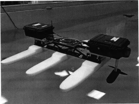
Figure 1: Kingfisher M 100m .. ... ... 8
Figure 2: Changes in pressure and velocity of the fluid ... 10
Figure 3: Propeller Pitch (Herbert, 2008)... 11
Figure 4: DC M otor Components ... 12
Figure 5: Inner armature mechanism ... 13
Figure 6: Propeller efficiency and the thrust and torque coefficients... 16
Figure 7: Torque derivation circuit schematic ... 17
Figure 8: Apparatus for measuring torque ... 18
Figure 9: Torque constant: Plotting current versus torque... 18
Figure 10: Torque constant verification: Angular velocity versus voltage... 19
Figure 11: Torque Speed Curves ... 20
Figure 12: Apparatus for measuring thrust ... 21
Figure 13: Thrust constant regression... 22
Figure 14: M otor Voltage Correlation ... 23
Figure 15: Propeller efficiency ... 24
Figure 16: Velocity Correlation... 25
Figure 17: Propeller efficiency with the model ... 26
1.
Introduction
Power consumption is a huge limitation in the application of autonomous vehicles, making the need for efficient processes more important. A greater operating efficiency would allow for a longer run-time or additional features by using less power for each existing mechanical process, extending the capabilities of the vehicle. This project is based on a dual-propeller autonomous surface vehicle primarily focusing on improving the operation of the propulsion
system. Through testing, a suitable range of propeller speeds will be obtained to that maximize the efficiency.
1.1 Objective
The objective of this thesis is to give a range of operating speeds for the Kingfisher M100' that will yield the highest efficiency in order to improve the time of operation. The resulting
information and analysis will allow the vehicles to be programmed to operate within these values, allowing for longer missions.
1.2 Organization
Following the introduction and objective, this thesis continues with a discussion of necessary background information that includes an overview of the vehicle's design, propulsion theory, propeller components, and direct current motors. This is followed with a derivation of the efficiency and what it signifies. The report continues with the following chapter, Experimental Design, which describes of how each variable was determined and relates to one another. The third chapter combines all of these results to show the operating efficiency of the vehicle. This report is concluded with the resulting implications of the findings.
1.3 Background 1.3.1 Vehicle Design
The vehicle used in this analysis of operating efficiency was a Kingfisher M100m, but the same process could be used for any other small surface vehicle. The Kingfisher M100M, created by Clearpath Robotics, consists of three hard-shelled, plastic flotation devices held together by a
sturdy, metal frame. Waterproof boxes are mounted on the starboard and aft sides of the vehicle, each consisting of a 12V battery, an amplifier, a control system, and leads to a motor mounted below, and are connected with waterproof Ethernet and power cords. The motors rotate a two-blade propeller with a diameter of 23cm and are rated to provide a maximum of 30 pounds of thrust force (133.4N) (Clearpath Robitics, 2011). The Kingfisher M100m can be seen in Figure 1. The aft box contains an antenna that can respond to a remote control, other Kingfisher M100m's, or a control console that remains on land to determine the vehicles course of action. Whichever device used to control the vehicles speed, turning, and direction sends a signal to each motor that determines the magnitude of the amplified voltage which ranges from around
-10V to +-10V. This means that each motor can have water flow through the front or back of the vehicle separately. For this analysis, a remote control with twelve forward settings for speed was used to control this signal. The remote control was pre-programmed to move both of the motors in unison for any action including turning.
1.3.2 Propulsion Theory
In order to understand the propeller efficiency, the relationship between propellers and propulsion has to be understood. In the past, there were two schools of thought that aimed to explain the behavior of propellers. The first only considered the change in velocity, and thus the change in momentum, of the fluid and the body as the source of the thrust force, but this was lacking as it did not include the dimensions of the blade itself. The second theory assumed that the propeller could be idealized as an actuator disk, which instantaneous increases the pressure of the fluid passing through it. The forces acting on the blade were then summed to yield a value for thrust. This allowed for the differences in the propeller to be included, but the assumptions
limited the theory's ability to model real world applications (Lewis, 1988).
The two schools of thought were later combined to create the Momentum Theory of Propeller Action that included the effects of the change in pressure and the change in velocity of the fluid. The theory still depicted the propeller as an actuator disk capable of raising the pressure once a fluid passes through it, with the magnitude of the rise dependent on the propeller dimensions. In reality, the propeller travels through the stationary fluid, but the propeller is represented as a stationary object with the fluid moving in the model. This is allowable because the dynamics are the same in both cases (Lewis, 1988).
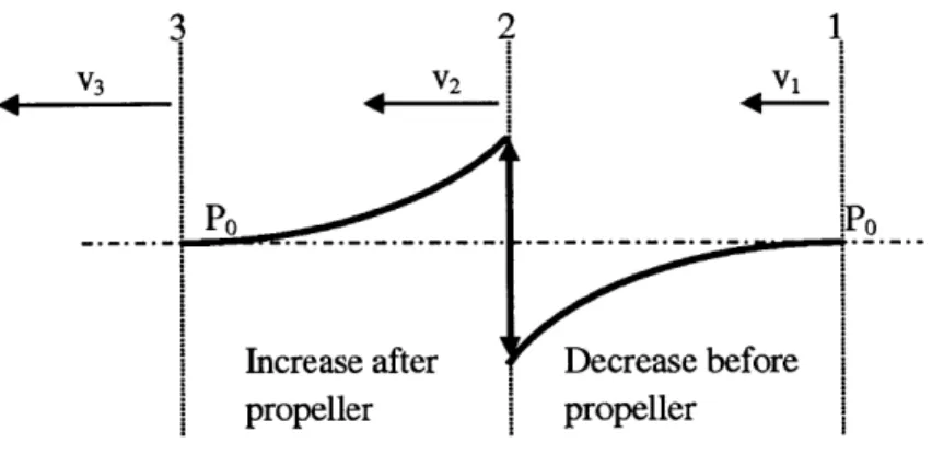
The theory is based on the dynamics of the fluid as it passes through three different cross
sections: 1) fluid flowing some distance in front of the propeller, 2) at the propeller, and 3) fluid flowing after some distance in front of the propeller. The fluid is originally at a known velocity and pressure at point 1) and ends at point 3) where it has travelled faster, but has returned to the same pressure. This rise in velocity does not occur instantaneously and increases gradually, meaning
V3 > V2 > V1 .
Bernoulli's formula states the energy of a fluid traveling on a streamline is equal to a constant value, meaning that a rise in velocity from point 1) to 2) will cause a drop in pressure because all other parameters are equal. The action of the propeller causes a spike in pressure immediately
after point 2), and gradually falls due to the same reason as before. This is shown more clearly in Figure 2 (Lewis, 1988). V-P0 Increase after propeller V1 Decrease before propeller
Figure 2: Changes in pressure and velocity of the fluid
The change in momentum per unit of time can then be used to find the thrust force with the velocities at points 1), 2), and 3). The mass of the fluid passing through the propeller in a unit of time is
m = pAV2,
where A is the cross sectional area of the disk the propeller creates during operation. This is then coupled with Newton's first law, which states
dv
F =m-, where
F = force on the body
m = mass of the body dv
- = Acceleration of the body. dt
In a unit of time, this becomes
F = m(v 3 - v1)
= pAv 2(v3 - v1). V3
As described earlier, the thrust force is dependent on the change in pressure and momentum (Lewis, 1988). The differences in propeller types determine the magnitude of velocities of the fluid as it passes through the propeller and the pressure increase.
1.3.3 Propeller Components
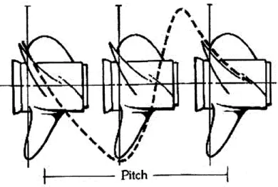
Delving further into propulsion theory, the thrust provided by propellers can be explained. Propellers are devices used to create a pressure and velocity increase in a fluid that passes through it as explained in the previous section. What differentiates propellers from one another is the ability it has to create this surge based on its physical design. The variation may be a result of the number of blades, pitch of the blades, or the diameter. All three characteristics affect the propeller's interaction with the water and its ability to change the momentum of the water to propel forward. Each blade is structured as an air foil and allows water to wrap around the leading edge in a uniform streamline, but creates a force that is related to the speed of the vehicle and direction of flow (Carlton, 1994). The force created can be broken down into a lift force, or propulsive force when used in this context, and a drag force that opposes the motion. The direction of flow relative to each blade has to do with the pitch, which is the distance the propeller would move forward in one revolution if it were not confined to the shaft, similar to a screw. This can be seen in Figure 3.
%
Pitch
In the practical sense, this value affects vehicles top speed and its maximum torque (Becker, 2011). The diameter and the number of blades affect the size of the surface that comes in contact with the fluid. This value can lead to a greater ability to affect the momentum of the fluid and improve the thrust force, but will create more drag force, causing a loss in top speed and torque.
1.3.4 Direct Current (DC) Electric Motor 1.3.4.1 Components and Inner Interactions
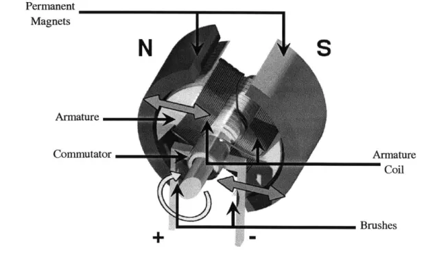
While this thesis is meant to analyze the propeller efficiency, it does not delve into the effects of changing the physical propeller. Instead, the analysis is performed on the operating conditions, meaning that the efficiency is dependent on the behavior or the motor that powers the propeller. The identical motors in the Kingfisher are brushed, commutated DC motors, which consist of two permanent magnets, an inner armature coiled with copper wire, a commutator, and bushes. The locations of these can be seen in Figure 4.
Permanent Magnets Armature Commutator Armature Coil Brushes
Figure 4: DC Motor Components (Hunter & Hughey, 2010)
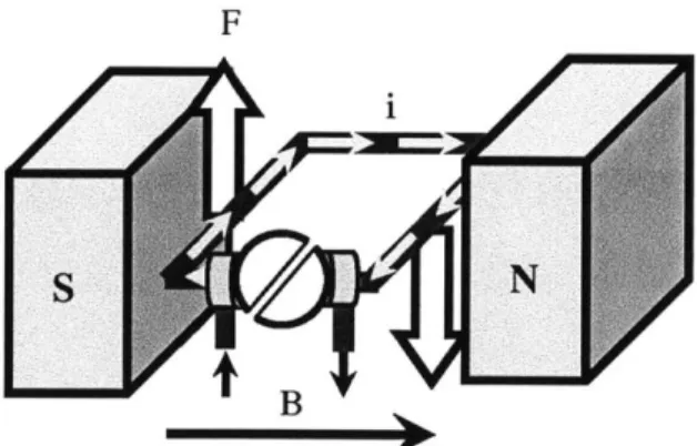
The opposite poles of the permanent magnets create a magnetic field originating from the south pole and ending at the north pole which interacts with the inner armature. Current travels through this armature coil, which magnetizes the armature and creates a Lorentz force. This is a
force exerted on a point charge in an electromagnetic field (Young & Freeman, 2008) and since current is the flow of charged particles through time, the relationship can be written as
F = L(i x B)
where
L = Length of the wire
i = Current
B = Magnetic field.
This relationship is fundamental in the workings behind a DC motor because the flowing current causes forces in opposite directions on each end of the armature, causing the entire object to rotate. A simplified version of this relationship can be seen in Figure 3. An uncoiled wire shows the forces that cause the armature to spin. The shaft is attached to the commutator, shown as the
split circle, whose purpose is to complete the circuit at all times and reverse the polarity of the loop when the armature makes a half revolution. Without this switch, the motor would not be able make a full rotation as the flow of current would cause the force to switch directions. The motor would continue to make half revolutions back and forth, but the commutator allows the direction of the current to change within the armature.
F
S N
B
Figure 5: Inner armature mechanism
As evident from the equation, the force causing the motor to rotate is dependent of the length of the wire, magnetic field, and the current. The current is the only one of the three that can vary, meaning a higher current will result in a greater spinning force and allow for greater angular velocities and torques.
1.3.4.2 Motor Parameters
Motors are often described by certain parameters that express their capabilities. Specifically, constants are often used to express relationships between easily measurable variables and those that are more difficult to record. The torque of a motor has been found to linearly relate to the rotation. Examples of these components include, but are not limited to, the size of the magnets, length of the coiled wire, and internal resistance. This relationship can be expressed as
T = Kri.
The thrust force provided by a motor/propeller combination is not often, if at all, compared with the current supplied, but by the same logic, the unchanging components/properties of the motor, propeller, and vehicle allows for a comparison to be made with the current (Hunter & Hughey,
2010). The relationships will be modeled by the regression that provides the best fit for the data.
1.3.4.3 Electromotive Force
The rotating movement of the armature not only causes the shaft to spin, it creates a back electromotive force, or back EMF, as per Faraday's Law (Young & Freeman, 2008). This electromotive force is actually a voltage that opposes the direction of the current, meaning the voltage provided by the power supply has to overcome the electromotive voltage created by the movement. The voltage produced is directly proportional to the speed of the armature coils, or the angular velocity of the shaft. This can be expressed as
EMF = KEMFI2
where KmF is a constant relating the two parameters and is equal to K, found in the previous section. As such, this angular velocity can be expressed in terms of the supplied voltage, V, armature resistance, R, and current, I, as
V -iR
KEMF
1.3.5 Efficiency
How effective a propeller is at drawing useful work from an input work is the definition of efficiency. In the case of the propellers on the Kingfisher M100TM, the input work is the torque necessary to rotate each propeller while the usable, output work relates to the thrust provided that
actually drives the vehicle forward (Sladky Jr., 1976) (Becker, 2011). Using non-dimensional analysis, each standard dimension (time, distance, and mass) was represented by the parameters that describe the system: angular velocity of the propeller, Q, diameter of the propeller, D, and the density of the fluid passing through, p. A different parameter was then combined with the standard parameters to create a non-dimensional relationship. The vehicle velocity, v, thrust force, T, and torque,
Q,
yield the advance ratio, thrust coefficient, and torque coefficient respectively using this non-dimensional relationship (Lewis, 1988). The final form can be expressed as: V Advance Ratio,J
= -T Thrust Coefficient, KT =pg2D4 pQ2 Torque Coefficient, Kq Qp2D5When these constants are combined, the propeller efficiency can be found as
j
KT2w KQ
which simplifies to time rate of change of the translational work over rotational work, or
v T
r7 = -.
21rf Q
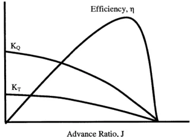
For most propellers, the torque and thrust coefficients are decreasing when plotted against the advance ratio, causing a maximum in the propeller efficiency seen if Figure 6. Advance ratios for vehicles large enough to transport people are able to travel faster than those used in this experiment and usually range from 0 to 1.2 and have peak efficiencies around an advance ratio of 0.7 to 0.8.
Advance Ratio, J
Figure 6: Propeller efficiency and the thrust and torque coefficients (Carlton, 1994)
2.
Experimental Design
In order to measure the efficiency of the propulsion system, relationships needed to be
established between variables that can be measured when the vehicle is in the water and those that cannot be determined. The onboard computer system is able to monitor the voltage supplied by the battery, the current traveling through the motor, and a position using a global positioning system (GPS). Of these, only the latter two are useful as the battery's voltage is not the same as the motor's voltage. For this reason, relationships need to be established to determine the torque, thrust force, and battery voltage for a given current.
2.1 Toque Derivation
The constant that relates the torque to the current needed to be found so that the torque provided would be known when the vehicle is in motion. To determine this relationship, the propeller was tested out of the water where the voltage was varied and the current and torque recorded. A
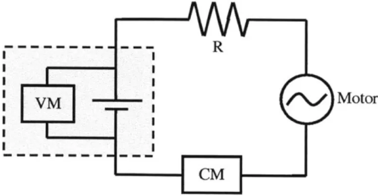
simple circuit was created to bypass the battery, amplifier and internal computer system so that a DC power supply could be used. This allowed for easier measurements as the power supply could monitor the current and the voltage at the same time. A secondary current sensor was
attached to the circuit just to check its accuracy. For better understanding, the circuit is shown below in Figure 7.
--- I R
VM /\/Motor
CM
Figure 7: Torque derivation circuit schematic
The grayed area represents the DC power supply as it provided the power for the circuit while also monitoring the values for current. The resistance of the system, R;, was found by using a multimeter and recording the displayed value.
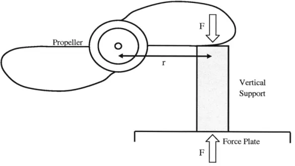
There are different ways to measure torque of a motor, but many of these methods were not applicable because the propeller could not be removed. The ideal method would be to use a Prony Brake where a chord is wrapped around the motor's shaft with measurable tensions so the difference would have been accounted for by the torque from the shaft, but this was not possible. Instead, the propeller's blade was used as a lever arm that pushed down onto a force plate as seen in Figure 8. The weight of the vertical support was taken into account as a fixed force that was negated by zeroing the scale. The support prevented the motor from rotating and a downwards force was exerted on the force plate. This force value was multiplied by the length from the center of the shaft to the contact point on the propeller to give the value for torque.
Vertical Support
Force Plate
Figure 8: Apparatus for measuring torque
The voltage supplied to the motor varied from 2.8V to 7V because the DC power supply was not able to operate at low voltage outputs or handle high current loads caused by the higher voltages. The results of can be seen in Figure 9.
Figure 9: Torque constant: Plotting current versus torque
After plotting the current versus the torque and running a linear regression, the constant was determined to be the slope of the line, or
1.8 1.6 1.4 -0' E 1.2 z 1' 0.8 0.2 0 0 10 20 30 40 50 Current (A)
Nm
K, = 0.0377 A2S
The boundary condition that holds this model is that the graph must originate from the origin because it is not possible for a torque to be generated without a current being applied, assuming frictional losses are negligible. The regression had a correlation coefficient, or R2 value, of
0.9094 meaning that it is a good fit of the data as a value of 1.0 corresponds to a perfect correlation.
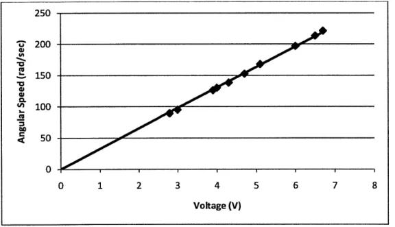
To confirm this constant, the voltage that corresponds to each of the data points was plotted against the no-load angular velocity, which is the maximum speed at a given voltage because of the absence of torque. The angular velocity was recorded using a digital tachometer and the data can be seen in Figure 10.
250 -200 150 a. 100 S50 0 0 1 2 3 4 5 6 7 8 Voltage (V)
Figure 10: Torque constant verification: Angular velocity versus voltage
With nearly a perfect correlation coefficient, the linear regression had an R2 value of 0.9985.
The slope of this line was 32.674, which was equal to the inverse of the motor coefficient, KEMF, or
1 Nm
KEMF = 32.674A2S
Nm
-The two comparable motor coefficients confirm that the DC motor is linearly correlated to the voltage and current, meaning there are no irregularities with the propulsion system as all DC brushed motors should ideally have equal coefficients.
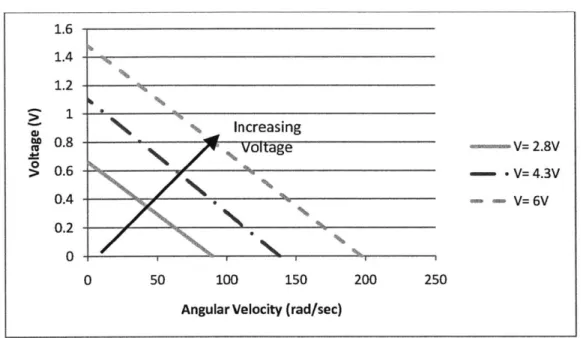
By combining the data from Figure 9 and 10, the stall torque and no-load speed of the propellers can be used to create torque-speed curves which show how the increasing voltage causes a parallel outward shift. What is important in this graph is that at a given voltage, there is a fixed tradeoff between the torque and the speed of the motor. While there is no intermediate data for at each, the endpoints are enough to create the curves.
1.6 1.4 -1.2' C0D Increasing 0.8 voltage - V= 2.8V 0.6 ---- -V= 4.3V 0.4 -- V= 6V 0.2 2 0 50 100 150 200 250 Angular Velocity (rad/sec)
Figure 11: Torque Speed Curves
2.2 Thrust Derivation
Just as with the torque, the thrust has to be modeled beforehand because it is not possible to measure this value when the vehicle is in motion. This model differs in that the vehicle was placed into the water because the thrust force is dependent on the density of the fluid passing through it, whereas the torque was generated from the motor itself.
A digital force sensor was clamped the back wall of an indoor testing tank with a depth of around four feet. A rope was fastened to the end of the sensor and tied to the metal frame of the vehicle. Enough distance was given in the rope so the wall would not interfere with the propellers as water needs to freely flow through. The current and tension in the rope was measured as the power supplied to the motors were varied using a remote control. During operation, the vehicle was not able to accelerate forward because it was bound by the rope, meaning all of the thrust force would be equal to the tension in the rope. There was some loss in accuracy as the vehicle would drift from side to side because this direction was not bound. A diagram of this can be seen in Figure 12. The key assumption in this test was that the motors had to be identical
because there would be no way to determine if one propeller provided more thrust than the other at the same operating current.
Thrust
Tension
Force
& Sensor
Thrust
Figure 12: Apparatus for measuring thrust
After halving the tension force to give the thrust for one motor, the results were plotted to determine if a trend could represent the relationship. The results are shown below in Figure 13.
Figure 13: Thrust constant regression
A linear regression was first used to model the data, but did not provide the best fit for the data. The regression used instead was a 2" order polynomial regression with an R2 value of 0.9164.
The thrust force of each motor was found to relate to current as follows: T = aTiz + bTi, where N aT = -0.1619 --A2 N bT = 6.6474- . A
This quadratic model was a good predictor of the data, but could not be extrapolated to explain higher currents because the trend would reach a maximum and begin to decrease. The propellers were rated to provide up to 301bf (133.4N) of force together, but this value was unobtainable because the maximum speed the vehicle was limited by the range of the joystick on the remote control. For this reason, the constants used for this model are limited in predicting values up until a current of 20.5A.
2.3 Motor Voltage 60 50 Z 40 20
10
F--OF0.
10 0 2 4 6 8 10 12 Current (A)The final relationship that had to be established was one between the motor voltage and the current. To measure the relationship, a voltmeter was attached to the motor while a current
sensor monitored the current leaving the motor. The vehicle was placed inside an indoor testing tank, where there would be greater control because of the calmer water. Using a remote control, the speed of the vehicle was varied, causing an increase in both the current and the voltage. The data was then logged and the regression that provided the best fit was used as a model. With an
R2 value of 0.9581, the 2" order polynomial regression edged out the linear regression that had
an R value of 0.9425. The results can be seen in Figure 14.
Figure 14: Motor Voltage Correlation The motor voltage was found under the
and can be expressed as
condition that the model had to pass through the origin
V = avi2 + byi, where av = -0.0155-A V b= 0.8944-. 10 9 8 7 on6 5 5 S 4 0 3 2 1 0 0 2 4 6 8 10 12 14 Current (A)
Like with the regression for the thrust force, this one cannot be extrapolated to explain higher currents because the trend will predict that the current will decrease which is not accurate. The model is limited in predicting the motor voltage up to 28.9A.
3.
Propeller EfficiencyIf the relationships found in Chapter 2 are assumed to completely describe the relationships that exist between the current passing through a DC motor and the torque, thrust, and voltage, the propeller efficiency can be found by monitoring the current and the vehicle's velocity.
A Kingfisher M100 TM was placed in the Charles River where a remote was again used to control the vehicle. The input provided by the remote control varied the vehicle's thrust from zero to full, forward power. The vehicle traveled for about twenty to thirty meters at the same speed so the surges in current from acceleration were not included. Variations occurring during these stretches were ruled out again by averaging the values at each setting. The motor current was monitored by the internal system and the speed was derived by using a GPS and differentiating it with respect to time. The efficiency was plotted against the advance ratio and is shown in Figure
15
Figure 15: Propeller efficiency
24 0.6 0.5-c. 0.4-W0.2 -0.1 4 0 0 0.02 0.04 0.06 0.08 0.1 Advance Ratio, J
As is now, the propeller efficiency is a function of the current and the velocity, meaning both variables need to be measured if one wanted to find the maximum efficiency. To simplify this process, another correlation can be established to allow the current to explain the velocity of the Kingfisher M100. Using the data from the GPS and the current recorded by the internal
system when the vehicle was not accelerating, the values can be plotted and analyzed using regressions as seen in Figure 16. In this case, a 3rd order polynomial regression was as chosen as
it had an R2 value of 0.9243, which was greater than the values for a linear, 2nd polynomial
regression. 2 1.8 1.6 1.4 1.2 -U 0 1 2 0.6 > 0.4 0.2 0 0 5 10 15 20 25 30 Current (A)
Figure 16: Velocity Correlation
As with the other regressions, this data cannot be extrapolated to larger values of current as it will produce inaccurate information, but can be expressed as
V = at, i3 + bvv i2 + c"'i where a, = 0.0002 m by, = -0.0137 s A2 -m c,, = 0.2615 -. s A
If extrapolated, the velocity would increase rapidly as the model is a 3rd order polynomial
is a correct measure of the immeasurable variable, the propeller efficiency can be modeled solely in terms of current, seen in Figure 17 with the data.
Figure 17: Propeller efficiency with the model
While the model is partly based on the data presented, it rightly shows a similar trend that an increasing efficiency occurs with an increasing advance ratio. What this data does show is only a
section of the efficiency diagram depicted in section 1.3.5. A maximum value was not obtained because not all of the advance ratios, which are based on vehicle velocity and angular velocity, were tested because it was not possible. The remote control and the motor itself are limited in how fast or slowly the propeller is allowed to spin. This means the condition where the propeller is spinning so fast that it is not able to take in as much could not be tested.
What is not seen in this data, but is shown in Figure 18, is that the higher efficiencies occurred when each motor was operating at the low levels of current. Each propeller spins at a low angular velocity, but proportionally provides more thrust than when a higher angular velocity is reached. 0.6 0.5 ~0.4 S0.3 0.1 -0 0 0.02 0.04 0.06 0.08 0.1 Advance Ratio, J
Figure 18: Efficiency expressed as a function of current
4.
Discussion and conclusion
The main take away from the data is that the maximum efficiency could not been determined because of the limitations in measuring and operating the propulsion system, but the most efficient operating condition occurred at low levels of current. The remote control did not allow for higher speeds to be obtained, but even if reachable, the motor might not have been able to handle the high currents necessary to rotate the shaft at these speeds.
The expectation was to find a suitable range of operation surrounding the peak efficiency. The data showed that the most efficient operating condition that outputted the greatest amount of thrust per torque inputted was to run the Kingfisher M100Tm at the lowest possible setting. While good in theory, this would be difficult in practice. The Kingfisher M100m's are designed to operate autonomous missions where they can collect data, using sensors, and coordinate with one another. Drastically lowering the vehicle speed would make the propulsion more efficient, but it may not be the best result overall because each autonomous mission would take a much
0.4 0.35 0.3 - 0.25 w 0.2 u' 0.15 0.1 0.05 0 0 5 10 15 20 25 30 Current (A)
longer time to accomplish. The tradeoff between runtime and the coverable distance that is created by varying the vehicle speed was not analyzed in this report.
Other improvements can be made to improve vehicle efficiency, but require physical changes. It is possible that the depth of the propeller has not been optimized as small vortexes are created behind the vehicle when it accelerates or runs at high velocities. If this was indeed an issue, lowering propeller would increase the flow of water and would improve the propeller's effectiveness of changing the fluid's momentum to create a thrust force. This could also be accomplished by adding a duct around the propeller in order to improve the fluid. A third option would to use a more powerful DC motor. When a propeller spins, the water creates a resistance torque that prevents the propeller from spinning as fast. This is demonstrated in Figure 11 where an increase in torque, water resistance in this case, would result in a decrease in angular speed at any given motor voltage. This means a motor with a lower KEAU would be better equipped to
5.
Works Cited
Becker, B. (2011). Understanding Propeller Pitch. Retrieved April 29, 2011, from Boating Magazine: http://www.boatingmag.com/maintenance/understanding-propeller-pitch
Carlton, J. S. (1994). Marine Propellers and Propulsion. Oxford: Butterworth-Heinemann. Clearpath Robitics. (2011). Clearpath Robotics: Kingfisher. Retrieved April 4, 2011, from Clearpath Robotics: http://www.clearpathrobotics.com/kingfisher
Herbert, J. W. (2008, August 12). Continuous Wave: Operations. Retrieved 4 28, 2011, from Continuous Wave: http://continuouswave.com/whaler/reference/manuall8-25/operations.html Hunter, I. W., & Hughey, B. J. (2010). DC Motor Characteristics Background. Cambridge: Staff of MIT Mechanical Engineering Department.
Lewis, E. V. (Ed.). (1988). Principles of Naval Architecture (3rd ed., Vols. II: Resistance, Propulsion and Vibration). Jersey City, NJ: Architects and Marine Engineers.
Sladky Jr., J. (Ed.). (1976). Marine Propulsion (Vols. OED-2). New York, NY: American Society of Mechanical Engineers.
Young, H. D., & Freeman, R. A. (2008). University Physics (Vol. I). San Francisco: Pearson Education.