Algorithms for three-dimensional free-form object matching

Algorithms for Three-Dimensional

Free-Form Object Matching

by

Kwang Hee Ko

B.S. in Naval Architecture and Ocean Engineering (1995) Seoul National University, Republic of Korea

M.S. in Naval Architecture and Marine Engineering (2001) M.S. in Mechanical Engineering (2001)

Massachusetts Institute of Technology

Submitted to the Department of Ocean Engineering in partial fulfillment of the requirements for the degree of

Doctor of Philosophy at the

MASSACHUSETTS INSTITUTE OF TECHNOLOGY June 2003

@

Author... ...

Department of Ocean Engineering March 13, 2003

C ertified b y ... ... ...

Nicholas M. Patrikalakis, Kawasaki Professor of Engineering Thesis Co-Supervisor

Certified by ...

Takasdi Maekawa, Principal Research Scientist Thesis Co-Supervisor

Accepted by.. ...

Michael S. Triantafyllou, Professor of Ocean Engineering Chairman, Departmental Committee on Graduate Students Department of Ocean Engineering

MASSACHUSETTS INSTITUTE OF TECHNOLOGY

AUG 2

5 2003

LIBRARIES

Algorithms for Three-Dimensional

Free-Form Object Matching

by

Kwang Hee Ko

Submitted to the Department of Ocean Engineering on March 13, 2003, in partial fulfillment of the

requirements for the degree of Doctor of Philosophy

Abstract

This thesis addresses problems of free-form object matching for the point vs. NURBS surface and the NURBS surface vs. NURBS surface cases, and its application to copy-right protection. Two new methods are developed to solve a global and partial match-ing problem with no a priori information on correspondence or initial transformation and no scaling effects, namely the KH and the umbilic method. The KH method es-tablishes a correspondence between two objects by utilizing the Gaussian and mean curvatures. The umbilic method uses the qualitative properties of umbilical points to find correspondence information between two objects. These two methods are ex-tended to deal with uniform scaling effects. The umbilic method is enhanced with an algorithm for scaling factor estimation using the quantitative properties of umbilical points. The KH method is used as a building block of an optimization scheme based on the golden section search which recovers iteratively an optimum scaling factor. Since the golden section search only requires an initial interval for the scaling factor, the solution process is simplified compared to iterative optimization algorithms, which require good initial estimates of the scaling factor and the rigid body transformation. The matching algorithms are applied to problems of copyright protection. A suspect model is aligned to an original model through matching methods so that similarity between two geometric models can be assessed to determine if the suspect model contains part(s) of the original model. Three types of tests, the weak, intermediate and strong tests, are proposed for similarity assessment between two objects. The weak and intermediate tests are performed at node points obtained through shape intrinsic wireframing. The strong test relies on isolated umbilical points which can be used as fingerprints of an object for supporting an ownership claim to the original model. The three tests are organized in two decision algorithms so that they produce systematic and statistical measures for a similarity decision between two objects in a hierarchical manner. Based on the systematic statistical evaluation of similarity, a decision can be reached whether the suspect model is a copy of the original model. Thesis Co-Supervisor: Nicholas M. Patrikalakis, Kawasaki Professor of Engineering Thesis Co-Supervisor: Takashi Maekawa, Principal Research Scientist

Acknowledgments

First of all, I want to thank my wife, Suyeon, for her love and emotional support, and my family for their love and understanding during my study at MIT.

I would like to thank my thesis supervisors, Professor Nicholas M. Patrikalakis and Dr. Takashi Maekawa, for their expert advice on my research work and instructive guidance on my academic studies, and Professors D. C. Gossard, H. Masuda, S. Sarma and F.-E. Wolter for their helpful advice as members of my doctoral thesis committee. Thanks also go to Professor Takis Sakkalis for his comments, Dr. Constantinos Evangelinos for helpful discussions and efforts for stable hardware environment for my thesis work, Mr. Fred Baker for efforts in the laboratory management, Design Laboratory fellows Dr. Wonjoon Cho, Ms. Hongye Liu, Mr. Da Guo and Mr. Harish Mukundan for making a good laboratory environment, and Dr. Yonghwan Kim, Mr. Jaehyeok Auh, Mr. Sungjoon Kim, Mr. Youngwoong Lee for their help and good advice.

Funding for this research was obtained from the National Science Foundation (NSF), under grant number DMI-0010127.

Contents

1.1 Background and Motivation . . . . 12

1.2 Research Objectives. . . . . 14

1.3 Thesis Organization. . . . . 14

2 Theoretical Background 16 2.1 Review of Differential Geometry . . . . 16

2.1.1 Basic Theory of Surfaces . . . . 16

2.1.2 Lines of Curvature . . . . 18

2.1.3 G eodesics . . . . 18

2.1.4 U m bilics . . . . 19

2.2 Review of NURBS Curves and Surfaces . . . . 22

3 Mathematical and Computational Prerequisites 25 3.1 Literature Review . . . . 25

3.1.1 U m bilics . . . . 25

3.1.2 Principal Patches . . . . 26

3.2 Rotation and Translation . . . . 27

3.3 Lines of Curvature . . . . 28

3.4 G eodesics . . . . 29

3.5 Orthogonal Projection of Points and Curves . . . . 31

3.5.1 Introduction . . . . 31

3.5.2 P oints . . . . 31

3.5.4 Lines of Curvatures . . . . 3.5.5 Geodesics . . . . 3.5.6 Calculation of Initial Values . . . . 3.5.7 Examples . . . . 3.6 Extraction of Umbilical Points . . . . 3.7 Shape Intrinsic Wireframing . . . . 3.7.1 Overall Structure . . . . 3.7.2 Algorithms for Constructing Quadrilateral Meshes . 3.7.3 Implementation . . . . 3.7.4 Analysis of the Algorithm . . . . 3.8 Interval Projected Polyhedron Algorithm . . . . 3.8.1 Robustness in Numerical Computation . . . . 3.8.2 Brief Review of Interval Projected Polyhedron 3.9 Conclusions . . . . Algor . . . . 33 . . . . 34 . . . . 35 . . . . 35 . . . . 36 . . . . 41 . . . . 41 . . . . 44 . . . . 46 . . . . 48 . . . . 48 . . . . 48 ithm . . . 49 . . . . 49 4 Object Matching 50 4.1 Literature Review . . . . 52 4.1.1 Moment Theory . . . . 52

4.1.2 Principal Component Analysis . . . . 53

4.1.3 Contour and Silhouette Matching . . . . 54

4.1.4 New Representation Scheme . . . . 54

4.1.5 Matching Through Localization/Registration . . . . 56

4.1.6 Miscellaneous Approaches . . . . 57

4.2 Problem Statement . . . . 59

4.2.1 Matching Objects . . . . 59

4.2.2 Distance Metric . . . . 59

4.2.3 Distance between a Point and a Parametric Surface . . . . 59

4.2.4 Distance Metric Function . . . . 60

4.3 Surface Fitting . . . . 60

4.4 Matching Criteria . . . . 60

4.4.1 E-Offset Test . . . . 61

4.4.2 Principal Curvature and Direction . . . . 61

4.4.3 Umbilic Test . . . . 61

4.4.4 Assessment of Matching . . . . 61

4.5 Moment Method . . . . 62

4.6 Correspondence Search . . . . 62

4.6.1 Algorithm using Umbilical Points . . . . 63

4.6.2 Algorithm using Curvatures . . . . 63

4.7 Algorithms with Uniform Scaling Effects . . . . 67

4.7.1 Use of Umbilical Points . . . . 68

4.7.2 Optimization . . . . 69

4.7.3 Complexity Analysis . . . . 71

4.7.4 Accuracy Analysis . . . . 72

4.7.5 Convergence of the Optimization Method . . . . 73

4.9 Conclusions . . . .

5 Shape Intrinsic Fingerprints

5.1 Introduction . . . . 5.2 Algorithms . . . . 5.2.1 Algorithm I . . . . 5.2.2 Algorithm 2 . . . . 5.3 Conclusions . . . . 6 Examples and Applications

6.1 Object Matching . . . . 6.1.1 Moment Method . . . . 6.1.2 Matching using Umbilics with Scaling Effects 6.1.3 Matching using Curvatures . . . . 6.2 Copyright Protection . . . . 7 Conclusions and Recommendations

7.1 Conclusions . . . . 7.2 Recommendations for Future Work . A Classification of Umbilical Points

A.1 Cubic Form . . . . A.2 Characteristic Lines vs. Cubic Form . . . . A.2.1 F: 0 -+

j(2e'

+e-iO

A .2.2 Jw J = 1 . . . . A.2.3 F2 : 0 -+ (2ei

0 _{+ e-2}0_{) . . . .}

A.3 Inverse Transformation . . . . B Formulation of Gaussian and Mean Curvatures

Bibliography 109 109 110 112 112 113 113 113 113 . . . . 114 115 117 . . . . 76 77 77 79 79 80 80 83 83 83 84 87 93

List of Figures

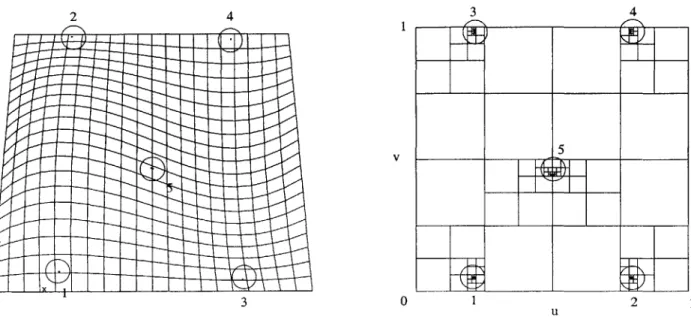
2-1 Three generic umbilics adapted from [91] . . . . 2-2 The umbilic diagram adapted from [96] . . . . 3-1 The orthogonal projection of a line of curvature . . . . 3-2 The orthogonal projection of a geodesic . . . . 3-3 An example of the adaptive quadtree decomposition (The marked dark domains indicate those which possibly contain umbilical points.) . . . 3-4 3-5 3-6 3-7 3-8 3-9 3-10 3-11 3-12 4-1 4-2 4-3 4-4 4-5

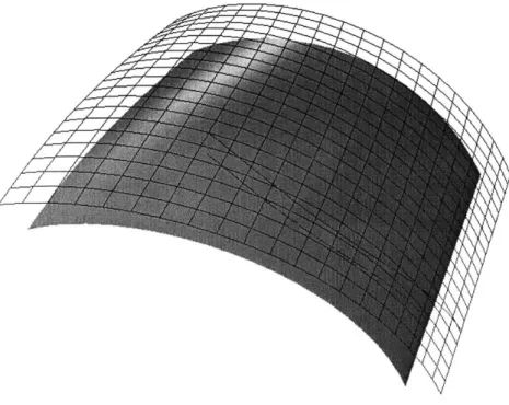
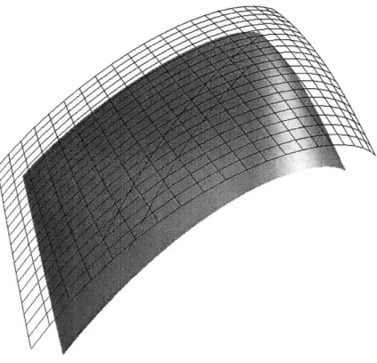
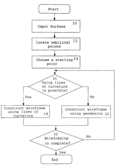
An example of isolated umbilical points on uv domain and th An example of a line of umbilical points . . . . Extraction of planar region . . . . A diagram of the algorithm . . . . Intersection of lines of curvature . . . . A diagram for meshing algorithm . . . . Intrinsic wirefram e . . . . A visual window for wireframing . . . . A control window for wireframing . . . . A diagram of the KH method . . . . (a) The Gaussian curvature (b) The mean curvature . . . . . A diagram for matching algorithm using umbilics. . . . . The surface used for the peformance test . . . . The approximated Gaussian and the mean curvature function

surface

graphs

5-1 Algorithm 1 for similarity decision . . . . 5-2 Algorithm 2 for similarity decision . . . .

6-1 6-2 6-3 6-4 6-5 6-6 6-7 6-8 6-9 6-10

Matching via integral properties . . . . . Surface rB and its umbilics . . . . Approximated surface rA and its umbilic

Umbilical points on the w-plane . . . . . Localized points on the surface . . . . . An example for global matching . . . . . Examples for partial matching . . . . A localization example of a hood . . . .

A matching example of a mask . . . . .

Initial position of the data points . . . .

20 22 36 37 38 40 40 41 42 43 44 45 46 47 64 66 70 75 75 81 82 . . . . . 84 . . . . . 85 . . . . . 86 . . . . . 86 . . . . . 88 89 . . . . . 90 . . . . . 91 . . . . . 92 . . . . . 93

6-11 The localized data points . . . . 94

6-12 An example showing that the ICP algorithm may fail. . . . . 94

6-13 An example for partial surface matching with scaling effects using the optimization method . . . . 95

6-14 A test surface and target points . . . . 96

6-15 Matching of a fictitious automobile hood surface . . . . 98

6-16 Comparison of lines of curvatures and umbilical points . . . . 99

6-17 (a) Weak test (E-offset) and (b) Intermediate test (maximum principal curvature) based on Algorithm 2 . . . . 99

6-18 (a) Intermediate test (minimum principal curvature) based on rithm 2 and (b) Intermediate test (principal direction) based on Algo-rithm 2 . . . . 100

6-19 Surfaces for the failure case . . . . 100

6-20 Wireframe of surface A . . . . 101

6-21 (A) c-offset (B) Maximum principal curvature (C) Minimum principal curvature (D) Principal direction . . . . 102

6-22 Umbilical points and lines of curvature . . . . 103

6-23 Case M1 : (A) c-offset (B) Maximum principal curvature (C) Minimum principal curvature (D) Principal direction . . . . 104

6-24 Case M2: (A) E-offset (B) Maximum principal curvature (C) Minimum principal curvature (D) Principal direction . . . . 105

6-25 Case M3: (A) c-offset (B) Maximum principal curvature (C) Minimum principal curvature (D) Principal direction . . . . 106

6-26 Wireframes for case M1, M2 and M3 . . . . 107

List of Tables

3.1 Comparison of positions of isolated umbilical points . . . . 39

4.1 Classification of matching problems . . . . 51

4.2 Degrees for integral and rational B6zier representations . . . . 65

4.3 Time comparison of two methods . . . . 76

6.1 Integral properties of solids A and B . . . . 83

6.2 Umbilical points in interval arithmetic . . . . 85

6.3 Umbilics and w values for rB . . . . .. . . . . . .. . . . . . 85

6.4 An umbilic and w value for rA . . . . 86

6.5 Angles and directions of lines of curvatures . . . . 87

6.6 Rotation angles for matching lines of curvature . . . . 87

6.7 Gaussian and mean curvature values for example 1 . . . . 87

6.8 Rotation matrix and translation vector for the hood . . . . 89

6.9 Rotation matrix and translation vector for the mask . . . . 90

6.10 Estimated rigid body transformation for the first example . . . . 91

6.11 Elapsed times for the examples . . . . 93

6.12 Statistical quantities for matching tests . . . . 93

6.13 Euclidean distances between the corresponding umbilics . . . . 95

6.14 Statistics for the matching tests . . . . 96

6.15 Quantitative similarity values . . . . 96

6.16 Statistics for the matching tests for case M1, M2 and M3 . . . . 97

6.17 The strong test for case M2 . . . . 97

6.18 The strong test for case M3 . . . . 98

6.19 Quantitative similarity values for case M1, M2 and M3 . . . . 98

List of Symbols

r surface

p point

u,v,t parameters

s arc length

I first fundamental form II second fundamental form

E, F, G first fundamental form coefficients

L, M, N second fundamental form coefficients t tangent vector

N unit normal vector K :normal curvature

K Gaussian curvature

H mean curvature

K9 :geodesic curvature

F' : Christoffel symbols

Ki,2 maximum and minimum principal curvatures

ri, r2 characteristic lines

W complex number for an umbilical point

V(x, y) cubic form

He (x, y) Hessian

w positive weight in a NURBS representation Bij :Bernstein basis function

Njj :B-spline basis function

6 tolerance

tT translation vector

R rotational matrix o4 :unit quaternion

de distance between two points

dst :minimum distance between a point and a surface 4D :global distance function

- : scaling factor Iij :moment of inertia

Chapter 1

Introduction

1.1

Background and Motivation

Rapid advance of computer technology has revolutionized design and manufacture of products in various fields. Almost all product data are created and stored in digital form using computer systems, and directly provided as input to computer aided manufacturing systems to produce physical products. As these data models are expensive and a significant part of the production process, there is a growing need to protect the ownership of these data models against unauthorized use by malicious parties [61]. Moreover, the ubiquitous nature of the Internet along with the World Wide Web and related technologies make it possible to rapidly exchange information electronically all over the world with no extra cost, which enables design and production to be performed at remote design and production sites. Easy data exchange, on the other hand, poses serious concerns to the owner of valuable data since such important data may be duplicated by unauthorized parties without losing any details when they are exposed to the Internet. Therefore, copyright protection for digital product models has become a major issue, and protecting intellectual property of digital information has emerged as an important research topic.

In the design and manufacturing fields, product models are typically represented in Non- Uniform Rational B-Spline (NURBS) form which is a standard format in industry [93, 89]. In the past, 3D model descriptions had been represented with a fairly restrictive shape variety, for example, 2D drawings (blueprints). Today they are typically described with CAD systems using digital data. Here the richest shape variety can be modeled by free-form surfaces that are typically defined as NURBS. Hence, the most important and fundamental part of the value creation process for a 3D model consists in creating the digital 3D free-form model.

Two types of feasible protection methods for 3D free-form objects can be consid-ered: one is to embed watermark information in the object and check the watermark for illegal duplication. The other method is to align two objects as accurately as pos-sible and check them for similarity. Several methods have been reported on digital watermarking for 3D models. Most of the methods are designed for models repre-sented via a triangular mesh or via range data. These techniques, however, are not

appropriate for 3D CAD data models usually represented in NURBS form. There has been an attempt to embed user-defined information to the NURBS representa-tion by Ohbuchi et al. [86]. But the embedded data can be easily destroyed by reparametrization or reapproximation. Since embedding robust user-defined water-marks in the NURBS representation is difficult, the similarity checking method can be adopted for protection of the ownership for digital objects represented in NURBS form.

Matching is a key step in the similarity checking method. The purpose of matching is to minimize the geometric discrepancy caused by translation, rotation and scaling. Three dimensional object matching has been one of the most important topics in com-puter vision, comcom-puter graphics and inspection, and there have been many significant contributions in developing matching methods for various representation forms such as NURBS surface patches, polyhedral surfaces and range data. Campbell and Flynn [20] regarded free-form as "a general characterization of an object whose surfaces are not of a more easily recognized class such as planar and/or natural quadric surfaces." Another interpretation was given by Besl [9]: "a free-form surface has a well defined surface normal that is continuous almost everywhere except at vertices, edges, and cusps." Many surfaces such as ship hulls, automobile bodies, aircraft fairing surfaces and organs are typical examples of free-form surfaces, which can be represented in various forms, such as NURBS surface patches, polyhedral surfaces and range data. Matching is used in various applications. The manufacturing process mostly uses matching techniques for automatic inspection, and in computer vision, matching is used for scene integration and object recognition. When matching is used in the con-text of computer aided inspection, it is referred to as localization [90], whereas when it is used in the context of computer vision it is referred to as registration

[10].

Many methods have been proposed for free-form object matching. In computer aided design, matching through minimization of a squared distance metric objective function is widely used since it is conceptually easy and shows good performance. But, such an approach cannot be used for a case that no a priori information for corre-spondence or initial transformation is provided, which commonly happens in practice. Correspondence information can be provided by the user and then an iterative search method can be employed to find the best transformation. In this case, however, the matching process is not automated. Partial matching and uniform scaling effects need to be considered in the context of the matching problem as well. Here, only uniform scaling is discussed since non-uniform scaling generally destroys the functionality of an object. A global method such as the moment method cannot handle partial ob-ject matching and most of matching methods fail to recover the scaling factor. A problem containing partial matching and scaling effects with no a priori information on correspondence is the most general form of the matching problem, which has not been studied so far.

1.2

Research Objectives

A primary objective of this thesis is to develop a global and partial matching method with scaling effects to handle the point vs. NURBS surface and the NURBS surface vs. NURBS surface cases when no a priori information on correspondence or initial transformation is provided. Two approaches are considered in this thesis: one involves use of isolated generic umbilical points and the other use of the Gaussian and mean curvatures and a ID optimization scheme. Using either one of them, two objects are aligned as closely as possible so that the differences between two objects caused by the rigid body transformation including scaling are minimized.

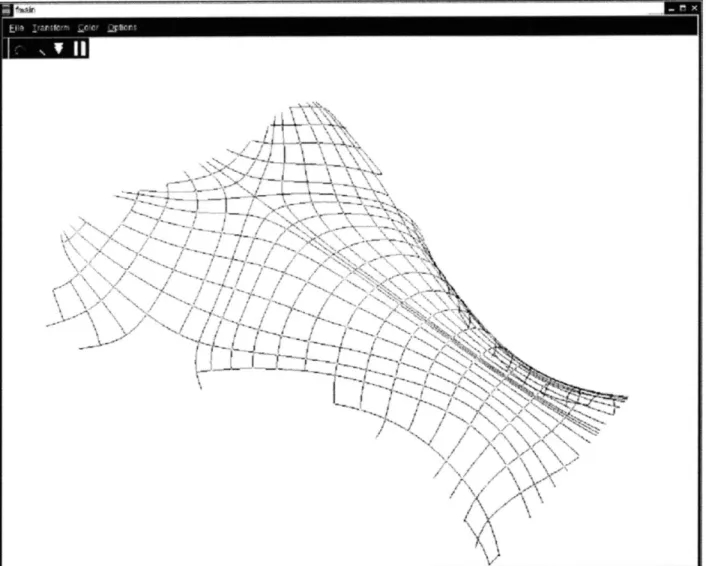
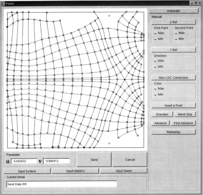
Efficient construction of shape intrinsic wireframe is another topic of this thesis. A shape intrinsic wireframe is a representation method of a surface using shape intrinsic properties, such as lines of curvature and geodesic curves which are independent of parametrization as well as the rigid body transformation. Robust calculation of the intrinsic properties is an important issue that needs to be considered in this thesis. Extraction of umbilical points deserves more attention because complete information on them is critical in construction of shape intrinsic wireframe, matching using um-bilical points and decision algorithms. An efficient and robust algorithm is developed to extract umbilical points from NURBS surfaces, which can effectively find not only isolated umbilics but also non-isolated umbilics forming curves or regions such as planar or spherical.

The assessment of matching is a topic that is also discussed in the thesis. Three hierarchical tests, the E-offset, principal curvature and direction test, and the umbil-ical point test, are proposed, and a quantitative evaluation method of similarity is developed along with two similarity decision algorithms. The algorithms consist of the three hierarchical tests, and produce systematic and statistical measures that can be used for a similarity decision.

Application of the proposed algorithms to copyright protection is demonstrated with examples. The decision algorithms are primarily used to determine if a suspect model is a copy of an original model. After matching the two models, a systematic and statistical assessment of the similarity between two models is performed, from which a decision can be made if one object is a copy of the other in a hierarchical manner.

1.3

Thesis Organization

The thesis is structured as follows:

In Chapter 2, differential geometry of surfaces, and the NURBS representation for curves and surfaces and their properties are reviewed. This is followed by mathemat-ical treatment of lines of curvature, geodesics and umbilmathemat-ical points. The classification of umbilical points is presented in detail.

In Chapter 3, computation methods and algorithms for lines of curvature, geodesic curves, orthogonal projection and extraction of umbilical points are presented. Using all proposed calculation methods, a quasi-automatic system to create surface intrinsic

wireframes is introduced.

Chapter 4 is devoted to matching algorithms. Two methods to establish a cor-respondence between two objects are proposed, and expanded to deal with partial matching problems with scaling when no a priori information on correspondence is given. One method involves use of umbilical points and the other use of an optimiza-tion scheme. Accuracy, complexity and actual performance analyses of the proposed algorithms are presented.

Two similarity decision algorithms are presented in Chapter 5, which are used for copyright protection. Both algorithms are based on the hierarchical tests proposed in Chapter 4. One algorithm uses the maximum values for a decision and the other provides statistical data for a decision.

Chapter 6 presents examples of the proposed matching algorithms and applications to protection of intellectual property.

Chapter 7 concludes the thesis with recommendations for future work.

Finally, detailed mathematical treatment of the classification of umbilical points is presented in Appendix A followed by brief presentation of the formulation of Gaussian

Chapter 2

Theoretical Background

In this chapter, mathematical definitions and concepts which will be used through-out this thesis are presented. Relevant aspects of differential geometry of surfaces are summarized [113, 32], and properties and classification of umbilical points are discussed in detail [95, 96, 17, 8, 79, 74, 91]. This chapter concludes with a brief discussion of definitions and properties of NURBS curves and surfaces [93, 50, 91].

2.1

Review of Differential Geometry

2.1.1

Basic Theory of Surfaces

A parametric surface can be defined as a subset of 3D space, R3, obtained by mapping a 2D parametric uv domain to R3

r(u, v) = [X(u, v), y(u, v), z(u, v)]T , (2.1)

where usually (u, v)

E

condition implies that a unique unit normal vector N is defined at every point on the surface and N = . A curve on a surface r can be represented in the form r(u(t), v(t)) where t is a parameter, usually in a range 0 < t < 1. The first

fundamental form, I, which is a distance measure on a surface, is defined as follows:

I = dr - dr = Edu2 _{+ 2Fdudv + Gdv}2_{, (2.2)}

where dr is infinitesimal displacement of a curve on a surface r(u(t), v(t)), and E =

-r F = r _{and G = r - L are the first fundamental form coefficients.}

9uO a u av av a

The second fundamental form, II, a measure of the curvature of a surface, is defined as follows:

II = -dr -dN = Ldu2 _{+ 2Mdudv + Ndv}2_{, (2.3)} where N is the unit normal vector of a surface, and L = N - j M = N. 2 _and

that if the normal curvature r, is positive, the center of curvature lies opposite to the direction of the surface normal. Here, N -! = N - r = 0 are used for the derivation. The unit tangent vector t of a curve on a surface r(u(t), v(t)) at p(E r) is obtained by differentiating r with respect to the arc length s, i.e. t = A. Then, the curvature_{ds~ n h uvtr} vector r, of the curve r(u(t), v(t)) at p can be calculated as the second derivative with respect to s, i.e.

dt d2_{r (2.4)}

ds ds2

The normal component of r., or K = - -N is the normal curvature of a surface r in

the direction of t at p. Equation (2.4) can be rewritten as [113]

dt dr dN _ II L+2MA + NA

2

,-.N= -N=---=-- -=(2)

ds ds ds I E+2FA + GA2 (.5)

where A = L. The extrema of , are obtained from = 0. This yields

(E + 2FA + GA2)(NA + M) - (L + 2MA + NA2)(GA + F) = 0, (2.6) which can be rewritten as:

(E + FA)(M + NA) (L + MA)(F + GA). (2.7) Therefore, equation (2.5) becomes

L+2MA+NA 2 M + NA L + MA

E+2FA + GA2 F+GA E+FA' (2.8)

from which we can set up two simultaneous equations to find the maximum and minimum principal curvatures and their directions:

(L+E)du+(M + F)dv = 0,

(M + F)du + (N + G)dv = 0. (2.9)

Equations (2.9) have non-trivial solutions if and only if

L+rE M+KF =0. _(2.10)

M+F N+KG

Two distinct real roots of (2.10), Ki and r 2 are the principal curvatures, and their corresponding directions A1 and A2 the principal directions [113]. The principal di-rections are orthogonal to each other. A double root r is obtained at an umbilical

obtained from the first and second fundamental form coefficients as follows [113]: LN - M2 K = B- 2 EG -F2' H I(2FM-EN-GL₂ EG-F2 (2.11)

2.1.2

Lines of Curvature

A line of curvature is a curve on a surface whose tangents are principal directions at all points on the curve. At a point on a surface away from umbilical points, two orthogonal principal directions are uniquely determined [113]. Hence, two lines of curvature (maximum and minimum) intersect orthogonally at such a point. Lines of curvature passing through an umbilical point are explained in Section 2.1.4.

Suppose that u = u(s) and v = v(s), where s is the arc length parameter. Then we obtain [113]

du

ds d ds = -= r(L + KE), (2.12)

if the first equation of (2.9) is used. Similarly, the second equation of (2.9) yields

du

ds dv -p(M + rF).ds (2.13)

Parametric values of lines of curvature are calculated by solving the first order differ-ential equations (2.12) or (2.13).

2.1.3

Geodesics

Let us define a unit vector u = N x t at a point p on a surface, where t is the unit tangent vector of a curve c on the surface at p. Then u is perpendicular to N and

t, and is contained in the tangent plane of the surface at p. The u component of the

curvature vector n of c, which is obtained by

K9 = (r. - u) u, (2.14)

is called the geodesic curvature vector, and

vature in the direction of t at p(E r) [113]. F k, (i, j, k = 1, 2) [113], 1 GE - 2FFu + FE 2(EG _{- F}2₎ r1l GEv - FGu 12 2(EG - F2_)' - 2GFv - GGu+ FGv 22 2(EG - F2_{) ,}

the magnitude of .9 is the geodesic

cur-Using (2.4) and the Christoffel symbols

F2 _{2EFu - EE + FE} S2( EG - F2) F2 _{EGu - FBE} 12 2(EG - _F2_)' 2 _EG, - 2FF + FGu 22 _{2(EG - F2} ) (2.15)

we can derive the geodesic curvature r, as follows: K = 9

[Pl

rli)

dv+

The equation of a geodesic curve can be obtained by setting K9 = 0 in equation (2.16)

according to the definition of the geodesics in [113]. Considering that the surface normal N has the direction of a normal tn to the geodesic curve, an alternative form of (2.16) can be obtained from equations n -r = 0 and n -rv = 0 using the Christoffel symbols k, (i, j, k = 1, 2) as follows [113]:_{+ i uv (v}

d 2u du 2 ds2 +rl ds) d 2 + p du 2 ds2 1 ds) Equations (2.17) equations [113]: du dv dv 2 + '2172 + F1 =0, ds ds ds 2du dv (dv 2 12t"s + ds ds -(2.17) (2.18) and (2.18) can be rewritten as a system of four first order differential

du ds dv ds dp ds dq ds (2.19) (2.20) (2.21) (2.22) = -FIp2 _{- 2l} 2p - 2, = -Flip2 - 2F 2pq - F 2q2.

2.1.4

Umbilics

An umbilic is a point on a surface where the normal curvatures in all directions are equal and the principal directions are indeterminate. The principal curvature functions are represented in terms of the Gaussian (K) and the mean (H) curvature functions as follows [113]:

Ki,2(u, v) = H(u, v) V/H

2_{(u, v) - K(u, v). (2.23)}

Let W(u, v) = H2 _{-K. The principal curvatures,}

K1,2 are real valued functions so that W > 0 must hold. From the definition of the umbilical point we have W(u, v) = 0. With these two conditions combined, we can infer that at an umbilical point, W(n, v) has a global minimum [72, 74]. Here, we assume that W is at least C2 smooth. Then, the condition that W has a global minimum at an umbilic implies that VW = 0. (2.16)

= A,

Therefore, at an umbilic the following equations hold [74]:

W(u, v) = , W(u,= 0

au

OW(u,

Ov

Given a polynomial parametric surface patch such as a rational Bezier surface

patch, we can set W = L-, where PN and PD are polynomials in both u and v.

With the condition W > 0, PN > 0 is assured since PD > 0 is always true under the regularity condition of the surface [113]. The equation W = 0 is equivalent to PN = 0. The first derivative of W is a = (%PNPD - PNaD)/PD(i = 1,2), where x, = u and x2 = v, which is reduced to 9 = (a'7)/PD using PN = 0. Therefore,

equations (2.24) are reduced to [74]

PN(u, v) = 0, =PN 0

O =

OPN 0.

Ov (2.25)

Classification of Umbilical Points

Umbilical points are classified into two types: generic and non-generic. Generic

umbilical points maintain their properties under small perturbations of the surface, while non-generic umbilical points may lose their qualitative properties under small perturbations [8, 104, 74, 91]. They can be isolated or form lines or regions. Isolated generic umbilical points are further classified into three types: star, monstar and

lemon as shown in Figure 2-1. Star type umbilical points are further classified into

-- - -- ! 1 77 "A7 Lemon -y 7 7 / / 7-/ / ~

~-i

Figure 2-1: Three generic umbilics adapted from [91]

the hyperbolic star and the elliptical star type umbilical points. The umbilical diagram shown in Figure 2-2 [96] is an easy way to distinguish the type of an isolated generic umbilical point. In order to use this diagram, the local surface near an umbilical point has to be represented as a height function or the Monge form with respect to a local coordinate system as follows [74]:

r = (x, y, h(x, y)). (2.26)

The height function h(x, y) is Taylor expanded at the origin of the local coordinate system. Then we have

h(x, y) = "(x2 +y 2

), (2.27)

2 13

+

I(a3

_0(4),

where r, is the normal curvature at the umbilical point. Let us set C(x, y) = axn3 +

3bx2_{y + 3cxy}2 _{+ dy}3_{. This expression implies that the local structure of a surface near}

an umbilical point is dominated by the coefficients of C(x, y), i.e. by a, b, c, d, which determine the type of umbilical points [79, 96]. It is convenient to represent the cubic part C(x, y) in the complex plane for analysis purposes. If we set ( = x + iy, then

C(x, y) becomes

C(()

where a = 0. We can express (2.28) in a coordinate system rotated about the normal vector without losing any essential features to make the coefficient of (3 equal to 1

[96]. Using = a3(, equation (2.28) becomes

C() = + 3 iJ k + 3w 2 _{+ 3, (2.30)}

where w = Oa- Z- . This means that C(x, y) is parametrized with respect to a

single complex variable w [17, 96]. Therefore, all variations of C(x, y) can be mapped onto the complex plane [17, 79, 96]. When a = 0, equation (2.28) is reduced to

C(() = 3(((0( + 0(). (2.31) This equation corresponds to infinity in the w complex plane [96, 17, 79], which is not considered in this discussion.

Depending on the structure of C(x, y) (or C(s)), three characteristic lines are determined as follows [96, 79]:

I F1 : 9 -+

j(2e"

* Iw|

F 12 : 0 -÷ (2eio + e-2M)

where F, and F2 are maps from 0 to the w complex plane. They divide the w complex plane into sub-regions as shown in Figure 2-2. Each sub-region corresponds to a specific type of an umbilical point. In Figure 2-2, ES means the elliptic star, HS

the hyperbolic star, MS the monstar and L the lemon. If w falls on a dividing curve, then the corresponding umbilical point is of non-generic type. The behavior of such an umbilical point can be analyzed with more higher order terms [74]. Using this diagram, the type of an umbilical point is easily determined, see [96, 17, 79]. A

L

_MS

_H

MS

S

ES

L

HS

L

Ms

F

Figure 2-2: The umbilic diagram adapted from [96]

detailed discussion on the characteristic curves is presented in Appendix A.

2.2

Review of NURBS Curves and Surfaces

A NURBS (Non-Uniform Rational B-Spline) representation is the most general form which includes integral B-spline and Bezier representations as special cases.

A NURBS curve q of order k is defined as follows:

Zo

q(u) = Z

OWiNi,kU)

i

weights, and Ni,k (u) the B-spline basis functions defined by

Ni, 1() = 1 Uif<<i+1

0 otherwise

Ni,k(u) = - Ni,k_1(u) + Ui+k - U (2.33)

Ui+k-1 - Ui Ui+k ui+1

with a non-uniform and non-periodic knot vector

U ={o, ui, I , Uk_1, Uk, Uk+1, - UP-1, I UP+1 , up+k,}, (2.34)

k equal knots p - k + 1 internal knots k equal knots

which has k + p + 1 elements. A NURBS curve has the following properties [93, 91]: " Geometry invariance property

" End points geometric property " Convex hull property

* Local support property

* Variation diminishing property

Similarly, a NURBS surface r of orders k and 1 and (m + 1) x (n + 1) control points is defined by

ET En~ wij RijNi,k (u) Nj, 1(v)

r(u, v ) N), 0 < u, v K 1 (2.35)

E= jy=o Wij Ni,k (U)Nj,l (V)

with non-uniform and non-periodic knot vectors U and V for u and v respectively,

U = {U,, Ui, - Uk, Uk1, ) ,Upi up-') up,, , , Up+k} k equal knots p - k + 1 internal knots k equal knots V = {VOVi,- ,Vi1, Vl,Vl+1, ... , Vq_,Vo ,V q+1< ,Vq+1}

1 equal knots q - 1 + 1 internal knots 1 equal knots

where Rij are the control points, wij the non-zero weights, and Ni,k and Nj,l the B-spline basis functions defined in (2.33). Most of the properties of NURBS curves are also applied to NURBS surfaces. However, the variation diminishing property is not applicable to NURBS surface patches.

The derivative of a NURBS curve q(u) or a NURBS surface r(u, v), however, is complicated since denominators need to be considered in the derivative calculation. Suppose that a NURBS curve is denoted as q ( and a NURBS surface .(uv). Then, the first derivative of q(u) with respect to u is given by

dq(u) N (Uq(u) D - qN (U) dq (U)

du Udu _(2.36)

The first derivative of r(u, v) with respect to u is given by

Or(u,

9u r(u, v)

Similarly, the first derivative of r(u, v) with respect to v is given by

ar(u,

BO r(uv)

The positive weight provides an additional degree of freedom to control the shape. If all weights are one, then the NURBS representation reduces to the integral B-spline representation. Geometric entities that the integral B-spline formulation cannot rep-resent such as conics (circle, ellipse and hyperbola) or quadrics, tori, cyclides, and surfaces of revolution [75, 93] can be modeled exactly using the NURBS representa-tion.

Chapter 3

Mathematical and Computational

Prerequisites

Intrinsic properties of a surface such as lines of curvature, umbilical points and geodesic curves, are full-fledged topics in differential geometry. Since they depend only on the geometry of a surface, they are independent of parametrization and repre-sentation methods, and invariant to the rigid body transformation such as translation and rotation. Because of such features, they have been widely used for matching and recognition purposes.

Accurate and robust evaluation of the intrinsic properties of a surface is important in order to use them in the applications. If a surface is represented in implicit, explicit or parametric form, then evaluation of the intrinsic properties is performed through analytic or numerical differentiation to yield exact values. In some cases, however, such evaluation alone is not enough depending on the applications. For example, calculation of umbilical points requires to solve a set of nonlinear polynomial equations which cannot be handled easily. In this case, the use of special tools is required.

This chapter is devoted to accurate and robust numerical calculation of various intrinsic properties which are used for matching and copyright protection explained in Chapters 4 and 5.

3.1

Literature Review

3.1.1

Umbilics

Umbilical points and the behavior of lines of curvature in the vicinity of umbilics have attracted the interest of many researchers. Berry and Hannay [8] classified the generic umbilics into three types, i.e. star, lemon and monstar, based on the coefficients of the cubic part in the Taylor expanded representation of a local surface and indices. They also showed the rarity of monstar patterns in the surfaces based on the statistical singularity theory. Porteous [95, 96] gave a thorough mathematical treatment of ridges and umbilics of surfaces, and Morris [79] studied ridges and sub-parabolic lines in particular. He also provided practical formulae for calculating

ridges and sub-parabolic lines with a bumpy cube as an example. Sander and Zucker [103, 104] studied a problem of extraction of umbilical points from 3D images and provided a computational method to identify umbilical points. An iteration scheme for a functional minimization under the compatibility constraints is used to refine the principal direction field and curvature estimates. The indices of the umbilics are calculated in the direction field to classify them.

Sinha [108] calculated differential properties of a surface represented in range data by using a global energy-minimizing thin-plate surface fit, and examined the effect of changing parameters in the surface fitting stage on the differential properties of the surface. Maekawa et al. [74] discussed a mathematical aspect of the generic features of free-form parametric surfaces, described a method to extract them, and investigated the generic features of umbilics and behaviors of lines of curvature around umbilical points on a parametric free-form surface. They presented novel and practical crite-ria which assure the existence of local extrema of principal curvature functions at umbilic points. The survey paper of Farouki [40] on various techniques for interro-gation of free-form parametric surfaces based on differential geometry, reviews the theories of surface curvatures, and provides an integration method for lines of curva-ture. Maekawa et al.

[74

3.1.2

Principal Patches

Principal patches are defined as the patches whose sides are lines of curvature [75, 76]. They depend only on the shape of the surface and are independent of the parametriza-tion or representaparametriza-tion methods. These properties have encouraged researchers to study them for use in computational geometry and CAD applications. Martin [75, 76] proposed a method for creating surface patches whose boundaries are lines of cur-vature. Two constraints, i.e. the frame and the position matching equations, are imposed on the boundary curves, which ensure that the boundary curves are lines of curvature and the surface normals of two adjacent patches along the boundary are the same so that the surface continuity is preserved. As a practical example for prin-cipal patches, Dupin's cyclides, which have circular lines of curvature, are taken and discussed, and Dutta et al. [38] used cyclides in surface blending for solid modeling. Sinha and Besl [109] reviewed mathematical aspects on principal patches and pre-sented an engineering solution to creating global principal patch networks. A meshing algorithm is proposed and the computational difficulties of building a quadrilateral mesh based on integrated lines of curvature are discussed such as isolation of planar and spherical regions, determination of directions of principal curvature, treatment of umbilics, etc. A concept similar to principal patches was proposed by Thirion [115]. He defined the extremal mesh as the graph whose vertices are the extremal points or umbilic points and whose edges are the extremal lines. The basic idea of the extremal mesh is the same as that of principal patches but he used a new local geometric invariant of 3D surface to resolve orientation problem arising in the construction of the mesh. Brady et al. [15] analyzed several classes of surface curves as a source of

constraint on the surface and as a basis for describing it, such as bounding contours, surface intersections, lines of curvature and asymptotes. The surface is smoothed out with appropriate 2D Gaussian masks which is based on convolution of the input data with a Gaussian function and then operators to estimate the first and second derivatives are used, leading to computation of the principal curvatures. Umbilics are detected based on the principal curvatures, and lines of curvature are extracted by minimizing a closeness evaluation function.

An umbilical point can be calculated from the fact that the principal curvatures at that point are equal. For a surface represented in analytical form, this produces a set of nonlinear system of equations which can be solved by using software tools such as Matlab. When a surface is provided as range data, application of the condition for umbilical point detection is not robust. A different approach needs to be introduced such as the index calculation after refinement of principal curvature fields, see Sander and Zucker [103, 104].

3.2

Rotation and Translation

Suppose that we have two 3-tuples mi and ni (i = 1, 2, 3), and correspondence information for each point. From these points, a translation vector and a rotation matrix can be calculated. The translation vector is easily obtained by using the centroids of each 3-tuple. The centroids cm and c, are given by

3 3

cm Mi Cn = ni, (3.1)

i=1 i=1

and the difference between cm and c becomes the translation vector tT = c" - cm. A

rotation matrix consists of three unknown components (the Euler angles). Since the two 3-tuples provide nine constraints, the rotation matrix may be constructed by using some of the constraints. But the results could be different if the remaining constraints are used for the rotation matrix calculation [48]. In order to use all the constraints equally, the least squares method may be employed [48]. The basic solution by Horn [48] is described below. Suppose that the translation has been performed. Then what is left is to find the rotation matrix R so that

3 <' = ni - (Rmi)1 2 i=1 3 3 3 SZnd2 - 2 ni - (Rmi)

+

is minimized. Here, D = E ni - (Rmi) has to be maximized to minimize V. The problem can be solved in the quaternion framework. A quaternion can be considered as a vector with four components, i.e. a vector part in 3D and a scalar part. A rotation can be equivalently defined as a unit quaternion ( =

[cos

which represents a rotation movement around (ax, ay, az) by 6 degree. In the quater-nion framework, the problem is reduced to the eigenvalue problem of the 4 x 4 matrix H obtained from the correlation matrix M:

S11 + S22 + 833 823 - S32 S31 - s13 S12 - 821 S23 - 832 811 - S22 - S33 S12 + S21 S31+ s13 3

ZT

The eigenvector corresponding to the maximum which minimizes equation (3.2). An orthonormal from a unit quaternion q = [qo, qi, q2, q3] by

812 822 832 813 S23 S33 S12 - S21 S31 + s13 S23 + 832 833 - S22 - S11

1*

I

positive eigenvalue is a quaternion rotation matrix R can be recovered

q 2 +q2 _q2 _q2 q₀ + q - q R= 2(qlq2 + qoq3) 2(qlq3 - qoq₂) 2(qlq₂ - qoq3) 2 2 2 _ 2 q0 + q2 q1 -q3 2(q2q3 + qoq1) 2(q₁q₃ + qoq2) 2(q2q3 - q0q1) q2 + q -q 2 q2 q0 +3q 1 2 The procedure described above can also be applied to

corresponding point pairs are provided.

the case where more than three

3.3

Lines of Curvature

Depending on the size of the coefficients, (L+KE) and (N+KG), either (2.12) or (2.13) are selectively used to trace a line of curvature. Namely, if I(L + KE) < 1(N + KG)

,

we solve (2.12). Otherwise, solve (2.13) to avoid numerical instability [3].

The factors q and yu are determined by using the normalization condition of the first fundamental form. Since lines of curvature are arc length parametrized, the first fundamental form is reduced to

(du )2

dsl

dudv de2

+ 2F + G I-I

dsds \ds) = 1. (3.6)

Substituting (2.12) into (3.6), we can obtain 7 by +1

SIE(M + F)2- 2F(M + rF)(L + rE) + G(L + KE)2 (3.7)

Similarly, we can calculate /y by

1

= IE(N + KG)2- 2F(N +KG)(M + KF) + G(M + KF)2

(3.8) where

The choice of the sign of r7 and p is based on the following inequality [91] to maintain the direction of the solution path:

(

- ds au ds iDv' ds au ds av₁

(duP 9rP dvP &rP\ (du Or dv Or\ ds au ds Ov ds au ds Ov)

where r = r(u(s), v(s)) is a line of curvature on the surface r with respect to the arc length s and the superscript p means the previous step during the numerical integration of the governing equations. A well known numerical method such as Runge-Kutta method or Adams method is adopted as a solution scheme to the system of nonlinear ordinary differential equations, see

[911.

3.4

Geodesics

There are two types of geodesic problems which may arise in real applications: one is the initial value problem (IVP) and the other is the boundary value problem (BVP). For IVP, the fourth order Runge-Kutta method can be applied to (3.39) through (3.43). However, in most cases, a geodesic problem comes in the form of BVP. It is well known that the solution to IVP is unique, whereas BVP may have many solutions or no solution at all. Two methods, the shooting method and the relaxation

method, are available for the solution to BVP. The relaxation method is considered

more stable than the shooting method [70]. What follows is a brief discussion about the relaxation method and its application to the orthogonal projection of geodesic curves.

Relaxation Method [70, 98, 91]

The boundary value problem can be solved with the relaxation method. It approxi-mates ordinary differential equations (ODEs) with finite difference equations (FDEs) on mesh points in the domain of interest [98, 70]. It starts with an initial guess and then iteratively converges to the solution, which is called to relax to the true solution [98]. Many schemes can be used to represent ODEs in the form of FDEs. In this work, the trapezoidal rule is adopted [70].

Let us assume that we have a first order differential equation as follows:

dy_

dx = g (x, y). (3.9)

dx

At two consecutive points k and k - 1, the trapezoidal rule turns equation (3.9) into

1

Yk - Yk-1 - (xk -- 1) )(gk(xk, Yk) + gk_1(xk_1, Yk-1)) = 0. (3.10) 2

treated as a single differential equation. Suppose that

y = (yiy2, -.. - - , y), g = (g1, 92, - - -gn)T,

a = (ai, a2,'* * Ian )T ) = (01,12, 2 -. - ,n )T. (3.11)

Then, a system of first order differential equations with two boundary conditions at A and B is given as follows:

dy = g(s, y), y(A) = a, y(B) = 3, (3.12)

ds

where s C [A, B]. Equivalently, the vector equation (3.12) can be represented in the finite difference form using the trapezoidal rule as follows:

Yk - Yk-1 1

= - [Gk + Gk_1], k = 2, 3,... ,m, (3.13) Sk - Sk-1 2

with boundary conditions

Yi=a, Ym=13, (3.14)

where a mesh of points satisfying A = si < S2 <- < sm = B is considered. Here,

the n-vectors Yk and Gk are discrete approximate values of yk(Sk) and gk(Sk). Let us refer to equation (3.13) as

Yk- Yk 1 Fk = (F1,k, F2,k, -* - -, F-, = Yk-1 [Gk + Gk_1] = 0, k = 2,3, , m sk - sk-1 2 (3.15) and equations (3.14) as F1 = (F1,1, F2,1, , 1)T = - a = 0, Fm+i = (Fi,m+i, F2,m+1,.-- , Fn,m+1)T = Ym - / = 0. (3.16) Then we have mn nonlinear algebraic equations

F = (F1,F ,- ,Fm+1)T = 0. (3.17)

The vector equation (3.17) can be solved by the Newton's iteration scheme.

For a more stable solution, a step correction procedure can be adopted as follows [70]:

y(i+) y() + PAY(0, (3.18)

where 0 < p < 1 is chosen so that ||AY(+)1 < ||Ay(0)1. Here |IAYH|1 is defined as:

|AYA|| = + + + ,(3.19)

k1 MU M, Mp Mq

where Mu, M., Mp and Mq are the scale factors for each variable. The values of

3.5

Orthogonal Projection of Points and Curves

Orthogonal projection is a well-known concept, and has many engineering and sci-entific applications. For example, in shipbuilding industry steel plates need to be trimmed off along pre-defined trimming lines before assembly [92], and in inspection of manufactured objects computation of orthogonal projection of measured points onto the CAD surface is a critical step [91].

The idea of the orthogonal projection of a point or a curve onto a surface proposed by Pegna and Wolter [92] is extended to include orthogonal projection of curves on a surface such as a line of curvature and a geodesic curve. Instead of discretizing lines of curvature or geodesic curves and then projecting the points, a set of differential equations is formulated, which directly trace the orthogonally projected curve using the concept of the orthogonal projection of a curve onto a surface by Pegna and Wolter [92].

In this section, a brief review of the orthogonal projection of a point and a curve by Pegna and Wolter [92] is provided followed by extension of the curve projection idea to the orthogonal projection of lines of curvature and geodesic curves.

3.5.1

Introduction

A few assumptions need to be made that a surface onto which a point or a curve is projected should be regular and second order continuous, a 3D curve remains close enough to the surface, and the projected point or curve lies in the interior of the surface. In this thesis, only a parametric surface r = r(u, v), (0 < u, v < 1) is

considered.

3.5.2

Points

The orthogonal projection of a point p onto a surface r is defined as a set of points such that

Q(p,

-~ q q(XqXq ) ZJ< .

(3.20) The existence of the orthogonal projection is not always guaranteed when the surface r has boundary, and more than one projected points may exist [92].

Formulation

The computation of an orthogonally projected point is easily done by Newton's method. Let us assume that p is a given point and q a projected point on a surface r.