Optical forward-scattering for identification of bacteria within microcolonies

HAL Id: cea-02528456

https://hal-cea.archives-ouvertes.fr/cea-02528456

HAL is a multi-disciplinary open access archive for the deposit and dissemination of sci-entific research documents, whether they are pub-lished or not. The documents may come from teaching and research institutions in France or abroad, or from public or private research centers.

L’archive ouverte pluridisciplinaire HAL, est destinée au dépôt et à la diffusion de documents scientifiques de niveau recherche, publiés ou non, émanant des établissements d’enseignement et de recherche français ou étrangers, des laboratoires publics ou privés.

Optical forward-scattering for identification of bacteria

within microcolonies

Pierre Marcoux, Mathieu Dupoy, Antoine Cuer, Joe-Loïc Kodja, Arthur

Lefebvre, Florian Licari, Robin Louvet, Anil Narassiguin, Frédéric Mallard

To cite this version:

Pierre Marcoux, Mathieu Dupoy, Antoine Cuer, Joe-Loïc Kodja, Arthur Lefebvre, et al.. Opti-cal forward-scattering for identification of bacteria within microcolonies. Applied Microbiology and Biotechnology, Springer Verlag, 2014, 98 (5), pp.2243-2254. �10.1007/s00253-013-5495-4�. �cea-02528456�

Optical forward-scattering for identification of bacteria within

microcolonies

Pierre R. Marcoux  Mathieu Dupoy  Antoine Cuer  Joe-Loïc Kodja  Arthur Lefebvre  Florian Licari  Robin Louvet  Anil Narassiguin  Frédéric Mallard

Pierre R. Marcoux (), Mathieu Dupoy

Department of Technology for Biology and Healthcare, CEA-LETI MINATEC, 17 avenue des Martyrs, 38054 Grenoble, France.

e-mail: [email protected] tel: +33 4 38 78 15 04

fax: +33 4 38 78 44 01

Antoine Cuer, Joe-Loïc Kodja, Arthur Lefebvre, Florian Licari, Robin Louvet, Anil Narassiguin

These authors contributed equally to this work.

Ecole Centrale de Lyon, 36 avenue Guy de Collongue, 69134 Ecully, France. Frédéric Mallard

bioMérieux SA, Innovation & Systems / Technology Research / Sample Prep & Processing Lab, 5 rue des Berges, 38000 Grenoble, France.

Abstract (150 to 250 words)

The development of methods for the rapid identification of pathogenic bacteria is a major step towards accelerated clinical diagnosis of infectious diseases and efficient food and water safety control. Methods for identification of bacterial colonies on gelified nutrient broth have the potential to bring an attractive solution, combining simple optical instrumentation, no need for sample preparation or labelling, in a non-destructive process. Here, we studied the possibility of discriminating different bacterial species at a very early stage of growth (6 hours of incubation at 37°C), on thin layers of agar media (1mm of Tryptic Soy Agar), using light forward-scattering and learning algorithms (Bayes Network, Continuous Naive Bayes, Sequential Minimal Optimisation). A first database of more than 1000 scatterograms acquired on seven Gram-negative strains yielded a recognition rate of nearly 80%, after only 6 hours of incubation. We investigated also the prospect of identifying different strains from a same species through forward scattering. We discriminated thus four strains of Escherichia coli with a recognition rate reaching 82%. Finally, we show the discrimination of two species of

coagulase-negative Staphylococci (S. haemolyticus and S. cohnii), on a commercial selective pre-poured medium used in clinical diagnosis (ChromID MRSA, bioMérieux), without opening lids during the scatterogram acquisition. This shows the potential of this method – non-invasive, preventing cross-contaminations and requiring minimal dish handling – to provide early clinically-relevant information in the context of fully automated microbiology labs.

Keywords Bacteria  Identification  Forward-scattering  Label-free  Microcolonies  Non-invasive technique

Introduction

There is an increasing need for rapid identification of contaminant and/or pathogenic bacteria for both industrial microbiological control and clinical diagnostics. In the particular field of infectious diseases management, most of the routine bacterial identification and antibiotic susceptibility testing still relies on 150 years old pasteurian methods based on bacterial growth and biochemical reactions. The manual systems based on biochemical testing, such as API strips (bioMérieux), chromogenic media (ChromID, bioMérieux / CHROMagar, Chromagar / Oxoid chromogenic media, ThermoFisher), are mature and robust and allow for handling a large variety of different samples in a simple and low-cost format. These methods, however, require at least one over-night culture step and are labor-intensive. Some of these methods have been or are being automated, be it at the level of characterization processes (Vitek2 system from bioMérieux / BDPhoenix from Becton Dickinson) or at the level of the full lab workflow (bioMérieux, BD Kiestra). This solves the issue of laboriousness while keeping the power of reference growth-based methods, but does not improve the time to results delivery. In response to that, faster analytical methods have been introduced. Genomic

analysis has been used as a means of identification or typing. For example, 16S ribosomal DNA sequencing is a standard method used for this task. Molecular biology techniques have proven to be sensitive down to a few molecules of characteristic nucleic acids, and can reach a very high specificity. Such methods are of particular interest for direct sample analysis, without any growth step. The advantage is a dramatic decrease of time to actionable results. However, in the perspective of routine testing in the more general case, such methods suffer for drawbacks of cost, dedicated infrastructures to prevent contamination issues, genetic plasticity and variability of targeted organisms, and sample preparation to deal with the complexity and variability of the wide variety of primary samples. Therefore, it seems wise to explore non-molecular methods that could use the strength of plate streaking for sample prep and provide clinically relevant and phenotype-related information starting from very low amounts of biological material after shorter growth times.

Several methods have been suggested for direct analysis of bacterial colonies, be it on-agar or with minimal colony handling. Among these, the most studied ones rely on spectroscopic techniques, such as mass-spectrometry (MALDI-TOF, DESI-MS) or optical spectroscopy (Raman, IR). Today, MALDI-TOF mass spectrometry is widely used (Fox 2006) as it provides very good identification performance compared to reference methods, more rapidly and at a lower global cost. The advantages that MALDI offers are minimal sample preparation, rapid results, very low reagent costs and a small amount of cells (105_{) required}

for identification. Alternatively, methods based on light scattering potentially have considerable advantage, since no sample preparation is required. Raman spectroscopy is based on collecting inelastic scattering emitted by a sample irradiated with a monochromatic excitation (laser). A typical Raman spectrum will comprise a number of Raman peaks which are indicative of the vibration modes of particular chemical bonds. The precise spectral position of these modes depends on the immediate environment of the probed chemical bond.

Therefore, Raman spectroscopy provides detailed information about the chemical composition of bacterial cells, which has been shown to be linked to bacterial identity down to the strain (Willemse-Erix 2009). Combined with optical microscopy (Raman microspectroscopy), this method can even be used directly on colonies growing at the surface of nutritive agar media, without any sample preparation and potentially on very small bacterial colonies. However, the Raman signal is usually very weak (Huang 2010 / only 1 in 106_-108 _{incident photons on the sample undergo Raman scattering). As autofluorescence is a}

thousand times more efficient phenomenon, Raman bacterial identification is very sensitive to growth media composition, especially in the case of chromogenic and fluorogenic media which contain many photoactive molecules or particles. In addition, recording a spectrum with a good signal-to-noise ratio requires between 10 seconds and several minutes, which severely limits the Raman technique for high-throughput bacterial identification.

Alternatively, methods based on light scattering potentially have considerable advantage over the previously mentioned methods, since they allow for direct on-agar analysis of bacterial colonies in a fast and truly non-invasive way. Today, two bacterial identification systems based on light forward-scattering are commercially available: either on planktonic cells in liquid culture (Haavig 2002, Micro Identification Technologies), or on millimeter-sized mature colonies growing on solid culture medium (Bae 2009, Advanced Bioimaging Systems). In the case of bacteria growing on agar, the system is based on the concept that variations in refractive indices and size, relative to the arrangement of cells in bacterial colonies, will generate different scattering patterns. The overall principle of colony analysis is to shine a laser beam (635 nm, 1mm beam diameter) onto mature (1.8 to 2 mm diameter) bacterial colonies and to analyse their forward scattering pattern. The BARDOT (Bacterial Rapid Detection using Optical scattering Technology) system developed at Purdue University was shown to provide precise identification of major foodborne pathogens (Bayraktar 2006).

Correct classification rates are in the 91-100% accuracy range (Banada 2007), within 5-10min analysis time, in an automated format (Bae 2009). Discrimination was performed at the genus and species level for Listeria, Staphylococcus, Salmonella, Vibrio and Escherichia with an accuracy of 90-99% for samples issued from food or experimentally infected mice (Banada 2009). Even though the BARDOT system provides faster identification than conventional plating methods or biochemical methods, the analysis throughput is limited by the incubation time of colonies that must be long enough to make them reach a certain size. For instance, E. coli and Salmonella species required 12h while Listeria needed 24-30h to meet the colony diameter criterion (Bae 2008, Banada 2009). Recently, some results were reported about the development of a µBARDOT new system, that is able to perform forward-scattering on microcolonies (colonies within 100-200 µm in diameter, incubation times between 7h and 12h), thanks to a 100µm-200µm beam diameter (Bae 2011). Thanks to colony profile measurements, quantitative correlations were plotted between the morphologies of studied microcolonies and their scattering patterns. However, this study focused on three species only and gathers few scattering patterns for each of them (between 10 and 20), which makes it harder to take into account variability within a given species. A study by Buzalewicz et al (2011) also investigated the correlation between colony structure changes and observed scattering patterns, for incubation times between 12 and 40 hours, but no attempt for identification has been made.

The aim of our study was to evaluate the discrimination power of elastic forward-scattering on micro-colonies, at both the species and strain levels. Thanks to an innovative optical setup, we could acquire the images of a given microcolony both in the direct space, in order to visualise its morphology, and in the reciprocal space (diffraction pattern). As a first step and working in well controlled conditions of culture and image acquisition, we studied the evolution of scatterograms of E. coli colonies along time between 5h and 10h of growth at

37°C. We show that growth times as low as 6h could be used for bacterial identification. For the acquisition of a scatterogram image library, we used this time seven Gram-negative strains on TSA for species-level comparisons, and four strains of E. coli for strain-level discrimination evaluation. We show here that our method allowed for good discrimination at both levels. Our system was tested in conditions close to clinical microbiology lab activity, using commercially available growth media and eventually in a non-invasive way, i.e. without opening the lid of Petri dishes. Starting from microcolonies of Staphylococcus cohnii and Staphylococcus haemolyticus growing on commercial Petri dishes of a medium commonly used in clinical diagnostic, we show the successful discrimination between these both coagulase-negative Staphylococci, although their visual morphologies looked very similar.

Materials and methods

Preparation of bacterial samples

Bacterial strains were obtained from the culture collection of bioMérieux (La Balme, France). They included Escherichia coli ATCC 25922 (arbitrarily called "EC10" according to our own procedures), Escherichia coli ATCC 8739 (called EC11), Escherichia coli ATCC 35421 (called EC21), Escherichia coli ATCC 11775 (called EC28), Hafnia alvei ATCC 13337 (called HA4), Citrobacter freundii ATCC 8090 (called CF7), Enterobacter cloacae ATCC 13047 (called EC8). Starting from a culture on TSA after 24h of incubation (37°C), a 0.5 McF suspension (Densicheck, bioMérieux) was prepared in suspension medium (bioMérieux). Agar media for the scattering experiments were prepared by filtrating melted TSA (Trypcase Soy Agar, bioMérieux, ref. 41 466) on a 0.2 µm membrane (Whatman 25 mm GD/X Sterile Disposable Filter 0,2 µm pore size). The filtrated agar medium is deposited onto a microscope

glass slide (50×22 mm; 170 µm thick), so as to obtain a 1 mm thick agar medium. The 0.5 McF suspension was then diluted at 1/1000 in suspension medium. 10 µL of the diluted suspension was finally plated on a 1-mm thick agar medium (TSA) deposed on glass (170 µm thick), in order to obtain approximately 102_-103 _{microcolonies on one slide. Cultures were}

incubated at 37°C for 6h in a humid chamber, so as to avoid desiccation of TSA medium. For the scattering experiments on CNS (coagulase-negative Staphylococci), S. cohnii and S. haemolyticus, a 0.5 McF suspension was prepared in a similar way, starting from a 24h-culture on TSA. Then 30 µL of a 1/1000 diluted suspension was plated on ChromID MRSA and incubated at 37°C for 6h.

Optical instrumentation

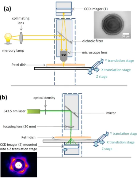
Our system is based on a Zeiss Axovision Microscope and includes the following major components (see Figure 1 for a schematic representation): a laser of 543.5 nm wavelength (5 mW power); two mirrors to adjust the laser beam and point it towards microscope; an x-y-z moving stage holding the Petri dish and positioning microlonies in the laser beam; two digital camera: one below for the acquisition of scattering patterns, and a second one (up) for the acquisition of images in the direct space, with a 50× magnification in order to get a precise image of the morphology of the microcolony; a beam splitter, so that we can chose between the acquisition in direct space or in reciprocal space. An attenuating filter reduces the laser power on bacteria down to 50 µW.

For the kinetic studies on E. coli (paragraph 3.1) and for the database on Gram-negative strains (3.2), a lens with a focal length of 100 mm was added to obtain a laser beam of 100 µm in diameter on the probed microcolony. For the experiments on CNS (3.3), a much shorter

focal length was chosen, 20 mm, so as to reduce the beam size on bacteria down to 25 µm and to match better the diameters of the laser beam to that of the typical microcolony.

Inoculated agar media were turned upside down so that bacteria were facing the camera recording scatterograms. In this way, no agar medium is on the optical path between the scattering object (the probed microcolony) and the imaging sensor. Scattering patterns are recorded with a monochromatic Pixelfly CCD camera, with a 1392×1024 resolution (pixels sizing 6.45 µm×6.45 µm). This camera was mounted on a linear translation stage along the vertical z-axis, so that we can adjust the distance between scattering object and imaging sensor from 10 mm to 42 mm. All the scattering experiments presented here were performed with a distance of 36.2 mm between microcolonies and sensor.

For every scatterogram, we chose an acquisition time as long as possible, so that we acquire high-order fringes with a good signal-to-noise ratio. At the same time, it had to be short enough to get an image without a single saturated pixel. As a consequence, time acquisition was usually adjusted between 0.4 and 1.2 ms. We noticed that the thicker is the microcolony, the more fringes are observed, the less intense is the transmitted beam and the longer the acquisition time can be.

Calculation of Zernike invariants

When it deals with comparing images quantitatively, one of the most common approaches is the transformation of images into row (or column) vectors. Each component Vi of a feature

vector V=(V1,…, Vi, …, Vn) is the projection of the image f(x,y) onto a basis function gi :











f

g

f

x

y

g

x

y

dx

dy

V

,

(

,

)

(

,

)

The choice of a set of basis functions is arbitrary (Chebyshev, Legendre, Zernike for example) and depends mainly on the symmetry properties of the images to be compared. As previously done by Bayraktar et al. (2006), we chose Zernike polynomials as basis functions. The Zernike moment Anm of the image f(x,y) is its projection onto the complex Zernike polynomial

Znm of order n and repetition m:











 

where: n is a natural number; m is an integer; for a given value of n, m varies from –n to +n with a +2 increment; the continuous image function f(x,y) vanishes outside the unit circle. Zernike polynomials, expressed in radial coordinates, have indeed interesting mathematical properties (Citti 2013). They are orthogonal over the continuous unit circle. All their derivative are continuous. They efficiently represent common errors (e.g. monochromatic eye aberrations) seen in optics. And finally they form a complete set, meaning that they can represent arbitrarily complex continuous surfaces provided given enough terms.

As the investigated microcolony is invariant on rotation around the optical axis, the application of Zernike moments to the analysis of bacterial scatterograms requires rotational invariance. That is why every scatterogram f(x,y) is represented by a feature vector V constituted by the magnitudes of Zernike moments (called Zernike invariants):

V =









 

Only values for positive m are computed since An,m  An,m and we decided to compute

Zernike invariants of up to 20th _{order. As a conclusion, the feature vector of a scattering}

pattern includes 120 components:

Zernike moments are used in many image processing applications involving pattern recognition because of their numerous qualities. However, they suffer from high computation cost. That is why many approaches have been developed to the fast computation of Zernike moments, such as recursive methods (Singh 2010, Gu 2002 and Chong 2003). In order to reduce the complexity of computation of the 2D-Zernike radial polynomials, we take benefits from their specific symmetry and anti-symmetry properties (Hwang 2006 and Wee 2006). In that way, we can generate the Zernike basis functions by only computing one quadrant, as illustrated in the Figure S1 and Figure S2 of the Electronic Supplementary Material. The supplementary files Zernn5m50.txt and Zernn5m51.txt are respectively the real and imaginary parts of an example of Zernike polynomial when m is odd (n=5, m=5). Zernn4m20.txt and Zernn4m21.txt are respectively the real and imaginary parts of an example of Zernike function when m is even (n=4, m=4). The other Zernike polynomials can be computed using the supplementary file defZern.m which is Matlab script.

In order to calculate Zernike invariants, we wrote a specific plugin for ImageJ software (Rasband 2013, Schneider 2012). This plugin, in java language, is available as a supplementary file (Zernike_.java). Briefly, the original images (1392×1024 pixels) are centred by placing 3 points on one of the circular fringes, usually the 1st _{order of the}

diffraction pattern. The centre of the unique circle that passes through these 3 points is considered later as the centre of the circularly shaped scattering pattern. A 1000×1000 rectangle is selected around this centre and the image is cropped. After subtracting the CCD offset, the greyscale intensity of each pixel is divided by the acquisition time in µs. Then the Zernike moments (n going from 1 to 20) are calculated on the unit disc sizing 1000 pixels in diameter:



(

,

)



,

1

)

,

(

1

_

_







y

x

dS

r

Z

y

x

f

n

A

_



where 4₂ N

dS is the elementary surface (N = 1000 is the diameter of unit disc in pixels). All pixels of the image within the unit circle have to be multiplied by the value of Zernike basis functions at the same location. For every pixel of coordinates (x,y), we calculate the product





)

,

(

)

,

(

x

y

Z

r



f

2 2 2 2 2                 x N y N N r and                             r N x N N y N Arc 2 2 2 2 tan 2  (6)

and by using a database of Zernike matrices plotting the value

Z

(

r

,



)

the unit disc. On an IntelCore i3 2.27 GHz with 2 Go RAM, computing the 120 invariants takes approximately one minute.

Data analysis

Multivariate data such as those from a scattering pattern consist of the results of observations on a number of individuals (objects, such as microcolonies) of many characters (variables, such as the Zernike invariants of the first 20th _{orders). Each variable may be regarded as}

constituting a different dimension, so that if there are p variables (invariants), each object may be said to reside at a unique position in p-dimensional hyperspace. This hyperspace is obviously difficult to visualise, that is why multivariate analysis is used, in order to summarise a large body of data by means of relatively few parameters, two or three if possible. In that way, a graphical display is possible, with a minimal loss of information, thereby allowing human interpretation. Among the variety of algorithms used in multivariate analysis, two main strategies can be distinguished: unsupervised learning, and supervised learning (Goodacre 2003).

Unsupervised learning

Unsupervised learning algorithms seek to answer this question: "How similar to one another are the objects (microlonies), based on the scatterograms I have collected ?" This approach is typically carried out using principal component analysis (PCA) or hierarchical cluster analysis (HCA). In the presented study, we have performed PCA, a well-known technique for reducing the dimensionality of multivariate data. The method consists of expressing the response vectors in terms of a linear combination of orthogonal vectors that account for a certain amount of variance in the data. The philosophy is indeed to find the best linear combination of variables that provides the most efficient clustering of classes. A thumb rule is that the number of identical samples necessary for the “training” of the algorithm should not be smaller than half the number of distinctive features (the first 120 Zernike invariants). That is why we acquired at least 100 scattering patterns for a given strain of the database. PCA analysis were performed using TANAGRA 1.4.48 data mining software (Rakotomalala 2005).

Supervised learning

A more powerful approach is to use supervised learning techniques, where one seeks to give answers to questions such as "Based on the scattering pattern of this unknown pathogen I have just collected, which class in my database does it (most likely) belong to ?" The basic idea behind supervised learning is that there are some scattering patterns which have desired responses which are known, i.e. the identity of known micro-organisms, decided by conventional approaches such as biochemical tests. These two types of data, the invariants of the scatterograms and their known identity, form pairs that are conventionally called inputs

(x-data) and outputs/targets (y-data). The goal of supervised learning is to find a model or mapping that will correctly associate the inputs with the outputs. In this way, if the algorithm has been trained on a sufficiently large database of pathogens, one can hope that any unknown bacteria sample will be efficiently recognised. If a new species is to be identified, we just need to add a few scatterograms to the database used for the learning step of the algorithm. Once recalculated on the newly extended database, the algorithm is able to recognise the new species.

As input of a given scatterogram, we used a row vector of 120 components, made of the Zernike invariants, and as output the corresponding strain. Supervised learning was done in a three-step process, following the cross-validation procedure of WEKA data mining software : 1. The constitution of a large database (between 110 and 132 scatterograms per strain), during which the amount of data was arbitrarily divided between a training set and a testing set. We had to ensure that, within a given class (HA4, CF7, EC8, EC10, EC11, EC21, EC28), the proportion of the training set was larger than the one of the testing set.

2. Then, as a second step, the algorithm could be trained. During that stage, the different parameters of the learning algorithm were calculated using the training set of each class. Three different learning algorithms of WEKA software (Hall 2009) were studied: Bayes Network, Naive Bayes and SMO (Sequential Minimal Optimisation).

3. Finally, as a last step, the testing sets were used to check the results of the learning algorithm, considering the outputs as unknown. The outcome was finally a confusion matrix, which makes it easy to see if the algorithm mislabels one class as another.

Bayes Network is a graphic probabilistic network built from a database of records, called cases. In this graph, nodes represent variables and arcs between nodes stand for probabilistic dependencies, based on the Bayes' theorem of conditional probabilities. Once probabilities have been found out thanks to the training set, such a network can provide insight into

probabilistic dependencies that exist among the variable in the database. It can also classify future cases of system behaviour by assigning a posterior probability. There are different ways of computing such a network; we used the K2 procedure, as described by Cooper et al. (1992).

Naive Bayes is a particular case of the last-mentioned Bayes algorithm. It is called "naive" because it is based on the strong assumption that the presence (or absence) of a particular feature (i.e. a given value of a variable) of a class is unrelated to the presence (or absence) of any other feature. In spite of their apparently over-simplified assumptions, Naive Bayes classifiers have worked quite well in many complex real-world situations (Langley 1992). Sequential Minimal Optimisation, or SMO, is a particular algorithm for training Support Vector Machines or SVM. In the case of SVM, each data point (i.e. scatterogram) is viewed as a vector in p-dimensional hyperspace (p=120 in our case). The goal of SVM is to separate vectors from different classes with a (p-1) dimensional hyperplane. The particular hyperplane that is chosen is the one that shows the maximum distance to the nearest data points. This specific hyperplane is called maximum-margin hyperplane and offers the largest separation between the two classes it separates. SMO has recently been designed to reduce calculation time of SVM, since large matrix computation is avoided (Platt 1998).

In order to test our trained learning algorithms, we used the "CrossValidateModel" procedure of WEKA software which is based on the validation method (Witten 2011). In cross-validation you decide on a fixed number n of folds, or partitions, of the dataset. Then the database is split into n approximately equal partitions: each in turn is used for testing and the remainder is used for training. We chose to compute a stratified tenfold cross-validation: nine-tenths were used for training and one-tenth for testing (n=10), and the procedure was repeated ten times so that in the end, every partition had been used exactly once for testing. Furthermore, the random sampling was done in a way that guaranteed that each class was

properly represented in both training and test sets: this procedure is called stratification and prevents from an uneven representation in training and test sets.

Results

Kinetic study on a given microcolony

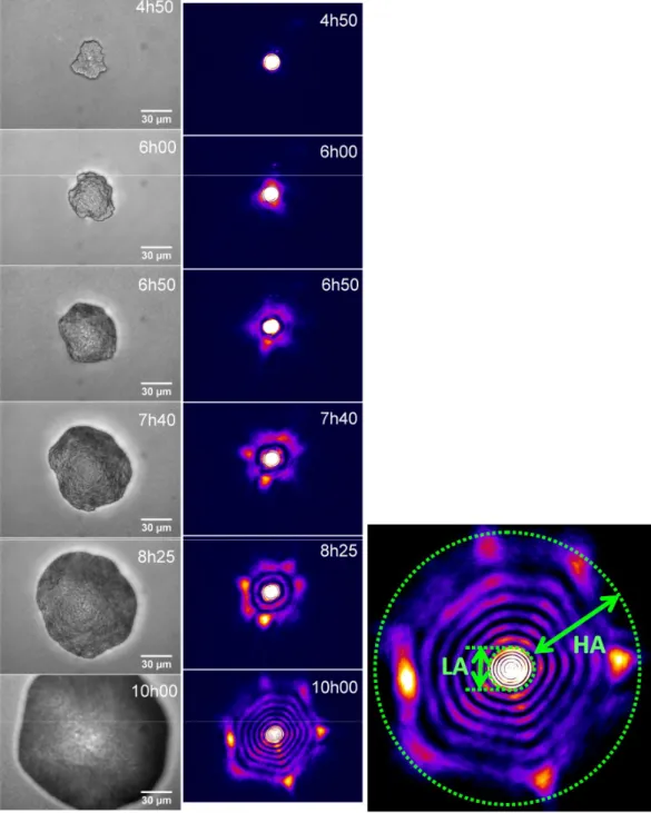
The experimental system used for this study (more details in the Materials & Methods section) is presented on Figure 1. Briefly, this system allows for both direct imaging of colonies and imaging of its scattering pattern (scatterogram). In order to find the best compromise between test time and informative power, our first step was to use this optical system to follow the link between scatterogram properties and direct space information during the early growth of bacterial colonies. Figure 2 illustrates the case of a given microcolony of E. coli EC28 (i.e. ATCC 11775) growing on TSA at 37°C, for incubation times ranging from 4h50 to 10h00. For every scattering pattern acquired in reciprocal space (right row in Figure 2), we also imaged the growing microcolony in direct space (left row).

Database after 6h of incubation on thin TSA medium

In order to assess the discriminating power of the method at the strain or species level, a set of different bacteria was used in well-controlled optical acquisition conditions. We chose species from different genera (Hafnia, Enterobacter, Citrobacter, Escherichia) within a same family (Enterobacteriaceae). The species we selected commonly colonize humans or are associated with human infections (Forbes 2007). The model included the Gram-negative species H. alvei (HA4), C. freundii (CF7) and E. cloacae (EC8) for species-level discrimination testing

(Figure 3) and four strains of the E. coli species (EC10, EC11, EC21 and EC28) for strain-level discrimination testing (Figure 4 and 5). All these strains grow on TSA agar medium, at 37°C for 6 hours. So as to minimise potential perturbations of light front-wave, bacteria were cultivated on a thin layer of agar medium with well controlled geometry (1 mm thickness), deposited on a 170 µm-thick glass slide. The acquisition of scatterograms was performed without any lid. In such growth conditions, we observed that microcolonies typically reach a diameter of approximately 100 µm (values ranged from 30 to 300 µm). That is why we adapted the laser beam to this typical size and all the database was acquired with this beam size. In order to take into account the colony-to-colony variability for each strain tested, we acquired more than 100 scatterograms for each condition.

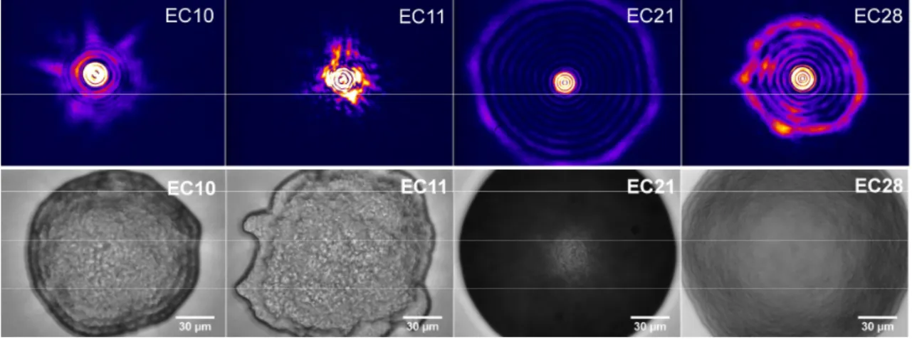
Scatterograms treatment and comparison were done as described in the Materials & Methods section, using a projection of each scattering pattern along the 120 first Zernike polynomials. 120-dimension vectors corresponding each to one given scatterogram were then classified using the three different learning algorithms described in Materials and Methods, so as to compare the confusion matrices and select the best performing approach. In this occasion, the SMO provided us with the best results (see the corresponding confusion matrix in Figure 3): an overall classification rate of 76.3% was obtained over the whole database. Now if we focus on the comparison between the four strains of E. coli, in direct space, we observed obvious differences about the ways bacteria stack within microcolonies (see Figure 4). These differences have a strong impact on the corresponding scattering patterns, as an acute classification can be reached with the chosen learning algorithm (see Figure 5): the confusion matrix displays an overall classification rate of 81.5%.

After performing the database after 6 hours of incubation on a thin layer of agar medium and without a lid, we wanted to assess the potential of the method to bring identification information in conditions close to the practice of real – potentially automated – clinical microbiology. The study was done in the frame of automated early reading of ChromID MRSA plates (bioMérieux, Marcy l’Etoile, France), which are commercial Petri dishes designed for the screening of methicilline-resistant Staphylococcus aureus (MRSA) carriers. We used our system and approach to investigate the distinction between two CNS strains able to grow on ChromID MRSA: a strain of S. haemolyticus, and another one of S. cohnii.

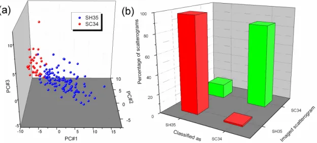
As Staphylococci grow more slowly than the Gram-negative species of the first database, we reduced the diameter of the laser beam down to 25 µm, so as to match better typical colony diameter and beam probe. Scattering patterns were acquired on ChromID MRSA after 6 hours of incubation at 37°C. After computing invariants, we performed unsupervised (see Figure 6a) and supervised learning (Figure 6b). The Naive Bayes learning algorithm yielded a classification rate of 92%.

Discussion

Kinetic study on a given microcolony

As previously observed by Bae et al. (2011) on a S. montevideo model, we noticed that the number of rings was increasing as the colony diameter increased. Furthermore, we observed that the low angle diffraction pattern, which is linked to low spatial frequencies (mm-sized objects), was detectable very early and was relatively stable over time, indicating that it may carry less information about bacterial parameters. This central part of the scatterogram can be attributed to scattering of the whole bacterial colony and may bring limited information about

bacteria themselves. On the opposite, the fringes at higher angles, corresponding to high spatial frequencies (i.e. much smaller objects like bacteria themselves) appear only after several hours of incubation (at least 4 to 6 h), are less intense, but their pattern is much more complex and was supposed to bring more discriminating information. Based on this, we finally made the decision to acquire the database of scattering patterns after 6 hours of incubation, and not earlier.

Database after 6h of incubation on thin TSA medium

The confusion matrix of Figure 5b shows, for this particular case of E. coli growing on TSA, the capacity of forward-scattering technique to discriminate, after only 6 hours of incubation, different strains of a same species. Information in reciprocal space, i.e. scattering patterns, is easier to collect than the one in direct space, i.e. microscopy images. Indeed, forward scattering does not require any microscope objective: a simple camera is enough.

Since computing the first 120 Zernike invariants is time-consuming (more than one minute per scatterogram), we tried to find out if some invariants are more relevant for the classification than others. In this respect, we observed over the whole database, E. coli and the other species, that the invariants of indices (0,0), (2,0), (4,0), (6,0), (8,0), (10,0), (12,0), (14,0), (16,0), (18,0) and (20,0) showed significantly higher values than the other invariants (their numbers are respectively 1, 3, 7, 13, 21, 31, 43, 57, 73, 91 and 111). All of them correspond to radial polynomials with a repetition m=0, i.e. real polynomials having a circular

symmetry (_eim 1_{). This suggests that these precise invariants carry most part of the} discriminating information.

This could be confirmed by calculating the Shannon entropy value for each of the 120 Zernike invariants over the whole scatterograms database (HA4, CF7, EC8, EC10, EC11, EC21,

EC28). This type of entropy was calculated using the entropy function of Matlab sotware and is defined as:



where X is a random variable with possible values {x1, x2, …, xn} and a probability

distribution p. It quantifies the unevenness of the probability distribution p (Lesne 2011). It can be viewed as the average unpredictability of the random variable X, which is equivalent to its information content. In particular, if we consider a variable with a determined outcome, the distribution probability will be fully localised in x0: p(x0)=1 and p(x)=0 for xx0, which

induces a minimal entropy H=0. On the opposite, for a given n, H is maximum and equal to log2 n when all the pi are equal (i.e. 1/n), which corresponds to the highest entropy and the

most uncertain situation (Shannon 1948). In that case, the random variable X does not convey any information. We computed the entropy H for every Zernike invariants (see Figure S3 of the Electronic Supplementary Material). For the 11 invariants described above, entropy is really low (under 0.06), whereas for all the other invariants H shows much higher values (above 3.33, up to 6.36). It may confirm that the invariants number 1, 3, 7, 13, 21, 31, 43, 57, 73, 91 and 111 bring more information than the others.

To estimate the level of performance that could be reached with this reduced set of Zernike invariants, we trained a learning algorithm and calculated the confusion matrix, in a similar way as what we did with the whole set of invariants in Figure 3. The overall classification rate has decreased by only 7.7%, which means therefore that most of the discriminating data are brought by these 11 invariants.

Infections caused by the genus Staphylococcus are of great importance for human health and cause a growing number of hospital-acquired infections (HAI). These Gram-positive cocci are divided into two major groups: CNS (coagulase-negative Staphylococci), such as S. epidermidis, and CPS (coagulase-positive Staphylococci), such as S. aureus. The latter can cause infections of the skin and other organs in immunocompetent patients, whereas coagulase-negative Staphylococci (CNS) comprise different species normally involved in infectious processes in immune-compromised patients, or patients using catheters.

Chromogenic selective media like the ChromID MRSA used in this study have become a key method for the rapid identification of MRSA in clinical samples (Morris 2012; Gazin 2012; Van Hoecke 2011). An antibiotic, such as cefoxitin, is added in order to discriminate methicillin-resistant S. aureus strains (MRSA) from the sensitive ones (MSSA). Unfortunately, a large number of CNS isolates are methicillin-resistant (Martins 2007) and thus grow on ChromID MRSA. To allow for the discrimination between resistant CNS and MRSA, chromogenic enzymatic substrates are used to detect the S. aureus-specific -glucosidase activity: direct identification of MRSA strains using ChromID MRSA is based on the green coloration of -glucosidase producing colonies in the presence of cefoxitin, while white or green-tinged colonies are disregarded as CNS isolates. The coloration, however, appears to be difficult to detect at early stages of colony formation: a 6h colony is hardly visible to the eye and the amount of coloured molecules is low. Hence, there would be a real interest in early distinction of MRSA without using enzymatic substrates. To show that forward scattering on microcolonies could satisfy this unmet need, we used our system and approach to investigate the distinction between two CNS strains able to grow on ChromID MRSA: a strain of S. haemolyticus, and another one of S. cohnii.

S. haemolyticus is the second most frequently isolated CNS from patients with hospital-acquired infections. It is part of the resident flora in the axilla, perineum, and inguinal areas of

humans. Most strains of S. haemolyticus exhibit a highly antibiotic-resistant phenotype, with a high MIC for methicillin (Garza-González 2010). S. cohnii is a novobiocin-resistant, coagulase-negative Staphylococcus that is known to colonize human skin; it has also been frequently identified in the hospital environment. The organism is typically methicillin-resistant (Vinh 2006) and frequently harbors plasmids mediating resistance to multiple other antibiotics.

These first results on the whole Petri dish, including lid, are very encouraging as the two Staphylococci species we studied are really close from a biological point of view. It brings the prospect of being able to distinguish MRSA from methicillin-resistant CNS after only 6 hours of incubation.

In the present study, we have shown the successful discrimination of bacterial microcolonies, only 6 hours after plate streaking. The discrimination can be done at the species- or strain-level. We also bring results suggesting that such discriminations might be done in real clinical microbiology lab conditions, using existing chromogenic media and in the context of fast automated plate screening.

Our results confirm that the ordered stacking of bacteria within colonies induces a periodic modulation of phase and absorbance in direct space that can be assessed using forward scattering imaging and used for bacterial classification. The important point in this study is that the colony-to-colony variability appears to be lower than the strain-to-strain variations in our restricted biological model, thus showing the possibility for a scattering-based identification system. Of course, there is no obvious reason why the scattering-based classification should be aligned on the biochemistry-based one. However, we show here that such a simple and low cost method can allow for very significant time saving in cases like MRSA screening, to the benefit of patients and hospital organization.

Elastic scattering yields much more photons, which allows for much shorter acquisition times than Raman technique. Besides being fast, the optical characterization we presented here is label-free, non invasive and non destructive. Furthermore, it can be done through a whole Petri dish, including lid, which prevents from cross-contamination. Finally, it does not require many cells and can be done on microcolonies having only 6 hours of incubation.

Acknowledgements

We are grateful to Frédéric Pinston, Quentin Jossso and Sylvain Orenga from bioMérieux for helpful discussions. Charles-Edmond Bichot (Ecole Centrale de Lyon) is gratefully acknowledged for assistance in java programming.

References

Bae E, Banada PP, Huff K, Bhunia AK, Robinson JP, Hirleman ED (2008) Analysis of time-resolved scattering from macroscale bacterial colonies. J Biomed Opt 13:014010. doi: 10.1117/1.2830655

Bae E, Aroonnual A, Bhunia AK, Robinson JP, Hirleman ED (2009) System automation for a bacterial colony detection and identification instrument via forward scattering. Meas Sci Technol 20:015802. doi:10.1088/0957-0233/20/1/015802

Bae E, Bai N, Aroonnual A, Bhunia AK, Hirleman ED (2011) Label-free identification of bacterial microcolonies via elastic scattering. Biotechnol Bioeng 108:637-644. doi: 10.1002/bit.22980

Banada PP, Guo S, Bayraktar B, Bae E, Rajwa B, Robinson JP, Hirleman ED, Bhunia AK (2007) Optical forward-scattering for detection of Listeria monocytogenes and other Listeria species. Biosens Bioelectron 22:1664-1671. doi:10.1016/j.bios.2006.07.028

Banada PP, Huff K, Bae E, Rajwa B, Aroonnual A, Bayraktar B, Adil A, Robinson JP, Hirleman ED, Bhunia AK (2009) Label-free detection of multiple bacterial pathogens using light-scattering sensor. Biosens Bioelectron 24:1685-1692. doi:10.1016/j.bios.2008.08.053 Bayraktar B, Banada PP, Hirleman ED, Bhunia AK, Robinson JP, Rajwa B (2006) Feature extraction from light-scatter patterns of Listeria colonies for identification and classification. J Biomed Opt 11:034006.

Buzalewicz I, Wieliczko A, Podbielska H (2011) Influence of various growth conditions on Fresnel diffraction patterns of bacteria colonies examined in the optical system with converging spherical wave illumination. Opt Express 19:21768-21785.

Chong CW, Raveendran P, Mukundan R (2003) A comparative analysis of algorithms for fast computation of Zernike moments. Pattern Recogn 36:731-742.

Citti G (2013) Zernike polynomials. University of Bologna (UNIBO), Mathematics Department. http://www.dm.unibo.it/home/citti/html/AnalisiMM/Schwiegerlink-Slides-Zernike.pdf. Accessed 4 April 2013.

Cooper GF, Herskovits E (1992) A Bayesian Method for the Induction of Probabilistic Networks from Data. Machine Learning 9:309-347.

Forbes BA, Sahm DF, Weissfeld AS (2007) Bailey & Scott's Diagnostic Microbiology, 12th

edn. Mosby Elsevier, St. Louis Missouri, p 324.

Fox A (2006) Mass spectrometry for species or strain identification after culture or without culture: past, present, and future. J Clin Microbiol 44:2677-2680. doi: 10.1128/JCM.00971-06 Garza-González E, Morfín-Otero R, Llaca-Díaz JM, Rodriguez-Noriega E (2010) Staphylococcal cassette chromosome mec (SCCmec) in methicillin-resistant

coagulase-negative staphylococci. A review and the experience in a tertiary-care setting. Epidemiol Infect 138:645-654. doi:10.1017/S0950268809991361.

Gazin M, Lee A, Derde L, Kazma M, Lammens C, Ieven M, Bonten M, Carmeli Y, Harbarth S, Brun-Buisson C, Goossens H, Malhotra-Kumar S (2012) Culture-based detection of methicillin-resistant Staphylococcus aureus by a network of European laboratories: an external quality assessment study. Eur J Clin Microbiol Infect Dis 31:1765-1770. doi 10.1007/s10096-011-1499-0

Goodacre R (2003) Explanatory analysis of spectroscopic data using machine learning of simple, interpretable rules. Vib Spectrosc 32:33-45. doi: 10.1016/S0924-2031(03)00045-6 Gu J, Shu HZ, Toumoulin C, Luo LM (2002) A novel algorithm for fast computation of Zernike moments. Pattern Recogn 35:2905-2911.

Haavig DL, Lorden G (2002) Method and apparatus for rapid particle identification utilizing scattered light histograms. US Patent, US2002/0186372A1. Micro Identification Technologies, http://www.micro-identification.com. Accessed 15 April 2013.

Hall M, Frank E, Holmes G, Pfahringer B, Reutemann P, Witten IH (2009) The WEKA Data

Mining Software : An Update. SIGKDD Explorations 11:10-19.

http://www.cs.waikato.ac.nz/ml/weka. Accessed 29 July 2013.

Huang WE, Li M, Jarvis RM, Goodacre R, Banwart SA (2010) Shining Light on the Microbial World: The Application of Raman Microspectroscopy. In: Laskin AI, Sariaslani S, Gadd GM (ed) Advances in Applied Microbiology, vol. 70, Academic Press, pp153-186. Hwang SK, Kim WY (2006) A novel approach to the fast computation of Zernike moments. Pattern Recogn 39:2065-2076. doi:10.1016/j.patcog.2006.03.004

Langley P, Iba W, Thompson K (1992) An analysis of Bayesian classifiers. In: AAAI-92 Proceedings of the Tenth National Conference on Artificial Intelligence, AAAI Press, pp 223-228.

Lesne A (2011) Shannon entropy: a rigorous mathematical notion at the crossroads between probability, information theory, dynamical systems and statistical physics. Institut des Hautes Etudes Scientifiques. http://preprints.ihes.fr/2011/M/M-11-04.pdf Accessed 2 August 2013. Martins A, Cunha MLRS (2007) Methicillin resistance in Staphylococcus aureus and Coagulase-Negative Staphylococci : epidemiological and molecular aspects. Microbiol Immunol 51:787-795.

Morris K, Wilson C, Wilcox MH (2012) Evaluation of chromogenic meticillin-resistant Staphylococcus aureus media: sensitivity versus turnaroud time. J Hosp Infect 81:20-24. Platt JC (1998) Fast Training of Support Vector Machines using Sequential Minimal Optimization. In: Schoelkopf B, Burges C, Smola A (ed) Advances in Kernel Methods – Support Vector Learning.

Rakotomalala R (2005) TANAGRA : un logiciel gratuit pour l'enseignement et la recherche. In Actes de EGC'2005, RNTI-E-3, vol. 2, pp.697-702. http://eric.univ-lyon2.fr/~ricco/tanagra/fr/tanagra.html. Accessed 25 March 2013.

Rasband WS. U.S. National Institutes of Health, Bethesda, Maryland, USA, http://rsb.info.nih.gov/ij/index.html. Accessed 5 April 2013.

Schneider CA, Rasband WS, Eliceiri KW (2012) NIH Image to ImageJ: 25 years of image analysis. Nat Methods 9:671-675.

Shannon CE (1948) A Mathematical Theory of Communication. Bell System Technical Journal 27:379-423, 623-656.

Singh C, Walia E (2010) Fast and numerically stable methods for the computation of Zernike moments. Pattern Recogn 43:2497-2506. doi:10.1016/j.patcog.2010.02.005

Van Hoecke F, Deloof N, Claeys G (2011) Performance evaluation of a modified chromogenic medium, ChromID MRSA New, for the detection of methicillin-resistant

Staphylococcus aureus from clinical specimens. Eur J Clin Microbiol Infect Dis 30:1595-1598. doi: 10.1007/s10096-011-1265-3

Vinh DC, Nichol KA, Rand F, Karlowsky JA (2006) Not So Pretty in Pink: Staphylococcus cohnii Masquerading as Methicillin-Resistant Staphylococcus aureus on Chromogenic Media J Clin Microbiol 44:4623-4624. doi:10.1128/JCM.01764-06

Wee CY, Paramesran R (2006) Efficient computation of radial moment functions using symmetrical property. Pattern Recogn 39:2036-2046. doi:10.1016/j.patcog.2006.05.027 Willemse-Erix DFM, Scholtes-Timmerman MJ, Jachtenberg JW, van Leeuwen WB, Horst-Kreft D, Bakker Schut TC, Deurenberg RH, Puppels GJ, van Belkum A, Vos MC, Maquelin K (2009) Optical fingerpriting in bacterial epidemiology: Raman spectroscopy as a real-time typing method. J Clin Microbiol 47:652-659. doi:10.1128/JCM.01900-08.

Witten IH, Frank E, Hall MA (2011) Data Mining: Practical Machine Learning Tools and Techniques. Morgan Kaufmann Publishers, 3rd _Edition.

Figure 1: The schematic of the optical set-up for imaging microcolonies both in (a) direct and (b) reciprocal spaces. (a) When imaging microcolonies in direct space, key components are: mercury lamp, dichroic filter and microscope objective. A first CCD imager records the corresponding image, as illustrated here with a microcolony of EC28 (E. coli ATCC11775), on TSA medium after 6h of incubation. (b) When acquiring scattering patterns, the source is coherent (laser) and the size of its beam is adapted through a focusing lens. It is strongly attenuated so as not to damage cells. The forward-scattering pattern is recorded below the Petri dish, thanks to a second CCD imager. The distance between the scattering microcolony and the CCD sensor can be adjusted.

Figure 2: Kinetic study on a given E. coli microcolony (EC28), between 4h50 and 10h00 of incubation on TSA agar medium at 37°C. Images were acquired both in direct (left row) and reciprocal (right row) spaces. On the close-up on the right, the boundary between the high-angle (HA) and low-high-angle (LA) patterns is outlined in green dashed points.

Classified as Imaged

scatterogram

E. coli

(EC10, EC11, EC21, EC28)

E. cloacae (EC8) H. alvei (HA4) C. freundii CF7 sum E. coli (EC10, EC11, EC21, EC28) 91.7 4.7 0 3.6 100% (468) E. cloacae (EC8) 45.7 44.9 0 9.4 100% (127) H. alvei (HA4) 0.8 0 86.8 12.4 100% (121) C. freundii (CF7) 6.1 6.1 6.1 81.7 100% (115)

Figure 3: Discrimination score at the species level: confusion matrix obtained with SMO learning algorithm, trained on the database gathering scatterograms of species grown 6 hours on TSA at 37°C. The columns (dark grey) indicate the predicted class and the rows (light grey) the actual class. For instance, the scattering patterns of HA4 were correctly classified as H. alvei species in 86.8% of cases. In 12.4% of cases, they were mislabelled as C. freundii and in 0.8% as E. coli. The overall classification rate is 76.3%.

Figure 4: Typical scatterograms (upper row, reciprocal space) and corresponding images (lower row, direct space; scale bars stand for 30 µm) for the four strains of E. coli, grown 6 hours on TSA at 37°C.

Figure 5: Unsupervised (a) and supervised (b) learning on the database gathering the scatterograms of the four E. coli strains. (a) Scattering patterns of the four strains of E. coli visualised in the first three principal components plot. (b) Confusion matrix provided by the SMO learning algorithm. The confusion matrix displays an overall classification rate as high as 81.5%.

Figure 6: Forward-scattering experiments with two CNS species, S. cohnii and S. haemolyticus, through commercial Petri dishes (ChromID MRSA), with closed lids, after 6h of incubation. (a) Scatterograms visualised in the first three principal components plot. (b)

Confusion matrix provided by the cross-validation of the Bayes Network learning algorithm (the average classification rate is 92%).

Applied Microbiology and Biotechnology

Electronic Supplementary Material for Optical forward-scattering for

identification of bacteria within microcolonies.

Pierre R. Marcoux  Mathieu Dupoy  Antoine Cuer  Joe-Loïc Kodja  Arthur Lefebvre  Florian Licari  Robin Louvet  Anil Narassiguin  Frédéric Mallard

Pierre R. Marcoux (), Mathieu Dupoy

Department of Technology for Biology and Healthcare, CEA-LETI MINATEC, 17 avenue des Martyrs, 38054 Grenoble, France.

e-mail: [email protected] tel: +33 4 38 78 15 04 fax: +33 4 38 78 44 01

Antoine Cuer, Joe-Loïc Kodja, Arthur Lefebvre, Florian Licari, Robin Louvet, Anil Narassiguin Ecole Centrale de Lyon, 36 avenue Guy de Collongue, 69134 Ecully, France.

Frédéric Mallard

bioMérieux SA, Innovation & Systems / Technology Research / Sample Prep & Processing Lab, 5 rue des Berges, 38000 Grenoble, France.

6 other supplementary files are provided with these instructions (Zernn4m20.txt, Zernn4m21.txt, Zernn5m50.txt, Zernn5m51.txt, defZern.m and Zernike_.java):

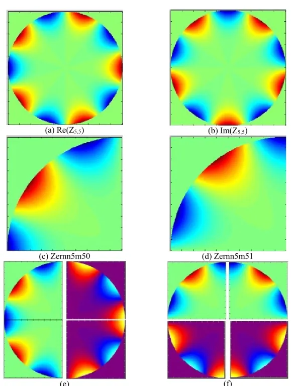
 Zernn5m50.txt and Zernn5m51.txt are respectively the real and imaginary parts of an example of Zernike polynomial when m is odd (n=5 and m=5 in this example). The first paragraph of these instructions (1.1 and 1.2) explains how the full Zernike function Z5,5 is computed starting from the two quartants Zernn5m50.txt and

Zernn5m51.txt, as illustrated in Figure S1.

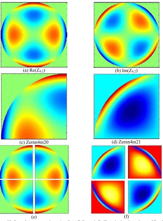
 Zernn4m20.txt and Zernn4m21.txt are respectively the real and imaginary parts of an example of Zernike function when m is even (n=4 and m=4 in this example), as illustrated in the Figure S2 of these instructions.

 The other Zernike polynomials can be computed using the Matlab script defZern.m, as explained in the first paragraph (1.3). The code of this script is also commented in this paragraph.

 After computing the Zernike polynomials forming the basis, the executable Zernike_.java computes the Zernike invariants of a given scatterogram. The second paragraph (2.1 and 2.2) explains how computation is coded and also how to install and run this java plugin (section 2.3).

1. Computation of Zernike polynomials

Zernike radial polynomials are expressed as follows:

  im nm nm r R r e Z ( , ) ( ) with:















Therefore, the plot of the imaginary part of a complex polynomial, Rnm(r)sin(m), is obtained by rotating the plot of the real part, Rnm(r)cos(m), with a

m 2



 angle.

In this chapter, we show how we calculate the value of Zernike polynomials Znm in every

pixel of the unit disc, so as to obtain two matrices: one plotting the real part of Znm, the other

plotting the imaginary part.

1.1 Symmetries of the real matrices

) cos( ) ( )] , (

Re[Z_n,m r R_nm r m (see Fig. S1) 1) x=0 axis: symmetry )] , ( Re[ ) cos( ) ( ) cos( ) ( )] , ( Re[Z_n,m r R_nm r m  R_nm r m  Z_n,m r 2) y=0 axis: symmetry or anti-symmetry, depending on the parity of m.

) 2 cos( ) ( ) 2 cos( ) ( )] 2 , (

Re[Z_n,m r    R_nm r m m R_nm r m m when m is even. ) 2 cos( ) ( ) 2 cos( ) ( )] 2 , ( Re[ ,       _{R r m m R r m m} r Znm   nm   nm  when m is odd.

1.2 Symmetries of the imaginary matrices

) sin( ) ( )] , (

Im[Zn,m r Rnm r m (see Fig. S2)

1) x=0 axis: antisymmetry )] , ( Im[ ) sin( ) ( ) sin( ) ( )] , ( Im[Z_n,m r R_nm r m R_nm r m  Z_n,m r 2) y=0 axis: symmetry or anti-symmetry, depending on the parity of m.

) 2 sin( ) ( ) 2 sin( ) ( )] 2 , ( Im[ ,       _{R r m m R r m m} r Znm   nm   nm  when m is even. ) 2 cos( ) ( ) 2 sin( ) ( )] 2 , ( Im[ ,       m m r R m m r R r Znm   nm   nm  when m is odd.

(a) Re(Z5,5) (b) Im(Z5,5)

(c) Zernn5m50 (d) Zernn5m51

(e) (f)

Figure S1. Case of an odd matrix: n=5 m=5. (a) Full matrix Re(Z5,5) plotting the real part of Zernike

function Z5,5 on the unit disc. (b) Full matrix Im(Z5,5) plotting the imaginary part of Zernike function Z5,5

on the unit disc. (c) We only compute this quartant of the real part Re(Z5,5) (file Zernn5m50.txt in the

"matrices" subfolder). (d) We only compute this quartant of the imaginary part Im(Z5,5) (file

Zernn5m51.txt). (e) The full matrix Re(Z5,5) can be reconstructed, starting from Zernn5m50 and using

symmetries. (f) The full matrix Im(Z5,5) can be reconstructed, starting from Zernn5m51 and using

(a) Re(Z4,2) (b) Im(Z4,2)

(c) Zernn4m20 (d) Zernn4m21

(e) (f)

Figure S2. Case of an even matrix: n=4 m=2. (a) Full matrix Re(Z4,2) plotting the real part of Zernike

function Z4,2 on the unit disc. (b) Full matrix Im(Z4,2) plotting the imaginary part of Zernike function Z4,2

on the unit disc. (c) We only compute this quartant of the real part Re(Z4,2) (file Zernn4m20.txt in the

"matrices" subfolder). (d) We only compute this quartant of the imaginary part Im(Z4,2) (file

Zernn4m21.txt). (e) The full matrix Re(Z4,2) can be reconstructed, starting from Zernn4m20 and using

symmetries. (f) The full matrix Im(Z4,2) can be reconstructed, starting from Zernn4m21 and using

symmetries.

1.3. DefZern program

The DefZern program (file defZern.m) is a Matlab script that uses the VZern function. It is used only once, in order to generate real Re



 





 



corresponding to the values of Zernike polynomials Zn,m

 



 



for Im



 



N=1001; Dimension of the square-shaped cropped image X0=(N+1)/2; Abscissa of the image centre

Y0=(N+1)/2; Ordinate of the image centre limmin=0; minimum value for n

limmax=20; maximal value for n

for n=(limmin:limmax) main loop, n varies between limmin and limmax

if(mod(n,2)==0) The parity of n is determined inf=0; The minimal value of m is calculated

mult=-1; Determination of the multiplying factor for m

else inf=1; The minimal value of m is calculated

mult=1; Determination of the multiplying factor for m

end

for m =(inf:2:n) Secondary loop, m varies between inf and n with a +2 increment Z=zeros((N-1)/2,(N-1)/2); Matrix is initialised

for x=(1:X0) Localisation loop, involving x

for y=(1:Y0) Localisation loop, involving y

r=2/N*sqrt((x-X0)^2+(y-Y0)^2); The radius of a pixel is calculated

if(r<=1) Condition: pixel is located within the unit disc

if(y==Y0&&x<X0) theta=pi;Calculation of  : case =π

elseif(y==Y0&&x==X0) theta=0;Calculation of  : case  =0

else Calculation of  : general situation, arctan of the half angle

theta=2*atan((2/N*(y-Y0))/(2/N*(x-X0)+r));

end

Z(x,y)=Vzern(n,m,r,theta); Computing pixel for real matrix

Zi(x,y)=Vzern(n,-mult*m,r,theta); Computing pixel for imaginary matrix

end end end

eval(['Zern.n' num2str(n) 'm' num2str(abs(m)) '=Z;']); Storing as Matlab files eval(['Zerni.n' num2str(n) 'm' num2str(abs(m)) '=Zi;']); Storing as Matlab files eval(['dlmwrite(''Zernn' num2str(n) 'm' num2str(abs(m)) '0.txt'',Zern.n'

num2str(n) 'm' num2str(abs(m)) ',''precision'',9)']); Stored as txt files

eval(['dlmwrite(''Zernn' num2str(n) 'm' num2str(abs(m)) '1.txt'',Zerni.n'

num2str(n) 'm' num2str(abs(m)) ',''precision'',9)']); Stored as txt files

end end

2. Computation of the Zernike invariants with the java

plugin

In conventional methods, all pixels within the unit circle have to be multiplied by the value of Zernike basis polynomials at the same location, and it has to be done first with the real part, secondly with the imaginary part. In our method however, the Zernike_.java program yields the Zernike moments using a quartant only of the basis functions (files Zernnimj0.txt and Zernnimj1.txt), thanks to the aforementioned symmetry properties of Znm radial functions.

2.1. Real matrices

First quadrant: original quadrant

for (int x = 0; x < N / 2; x++) {

for (int y = 0; y < N / 2; y++) {

intermediaire_calcul = intermediaire_calcul + (ip.getPixelValue(x, y) - offset) * matrix[x][y] * 4 / N / N / expTime; }

}

Second quadrant: symmetry or antisymmetry with respect to y axis

for (int x = N / 2 + 1; x < N; x++) { for (int y = 0; y < N / 2; y++) {

intermediaire_calcul = intermediaire_calcul + sym * (ip.getPixelValue(x, y) - offset) * matrix[N - x][y] * 4 / N / N / expTime; }

}

Third quadrant: symmetry or antisymmetry with respect to the origin point

for (int x = N / 2 + 1; x < N; x++) {

for (int y = N / 2 + 1; y < N; y++) {

intermediaire_calcul = intermediaire_calcul + sym * (ip.getPixelValue(x, y) - offset)

* matrix[N - x][N - y] * 4 / N / N / expTime; }

}

Fourth quadrant: symmetry with respect to x axis

for (int x = 0; x < N / 2; x++) {

for (int y = N / 2 + 1; y < N; y++) {

intermediaire_calcul = intermediaire_calcul + (ip.getPixelValue(x, y) - offset) * matrix[x][N - y] * 4 / N / N / expTime; } }

2.2. Imaginary matrices

First quadrant: original quadrant

for (int x = 0; x < N / 2; x++) {

for (int y = 0; y < N / 2; y++) {

intermediaire_calcul = intermediaire_calcul + (ip.getPixelValue(x, y) - offset) * matrix[x][y] * 4 / N / N / expTime; }

}

Second quadrant. Axis of symmetry: y axis (m is odd: symmetry; m is even: antisymmetry)

for (int x = N / 2 + 1; x < N; x++) { for (int y = 0; y < N / 2; y++) {

intermediaire_calcul = intermediaire_calcul - sym * (ip.getPixelValue(x, y) - offset) * matrix[N - x][y] * 4 / N / N / expTime; }

}

for (int y = N / 2 + 1; y < N; y++) {

intermediaire_calcul = intermediaire_calcul + sym * (ip.getPixelValue(x, y) - offset)

* matrix[N - x][N - y] * 4 / N / N / expTime; }

}

Fourth quadrant: antisymmetry with respect to x axis

for (int x = 0; x < N / 2; x++) {

for (int y = N / 2 + 1; y < N; y++) {

intermediaire_calcul = intermediaire_calcul - (ip.getPixelValue(x, y) - offset) * matrix[x][N - y] * 4 / N / N / expTime; }

}

The executable Zernike_.java was written as a plugin for ImageJ, a public domain Java image processing program. As a consequence, it must be placed in the plugins folder ImageJ/plugins/ before installing. The subfolder matrices gathering all the files Zernnimj0.txt and Zernnimj1.txt must be placed in this folder as well. As any ImageJ plugin, Zernike_.java must be compiled once before using it (Plugins  Compile and Run…).

After opening an image, simply run the plugin (Plugins  Zern  Zernike), the following window appears:

After filling these different fields (exposure time, offset value of the camera, etc.) another window comes out and asks "click on three points…". Then three points belonging to the same ring must be chosen (a zoom view can be activated with "+" key), so as to run an algorithm determining the unique circle that passes through these 3 points. This circle is displayed, as well as its centre, so that the user can validate it or not:

If "No" is chosen, three other points can be chosen on the same image, in order to restart the centring process, otherwise the cropped and centered image (1000 × 1000 pixels) appears and the calculation of invariants can start:

Once all the invariants are computed, a final window is displayed:

If "Yes" another image will be opened, so as to restart the process on a new image. If "No", plugin and image will be closed. The invariants are stored as an arff file, called Resultats_DATE.arff and located in the same subfolder as the selected images.

3. Shannon entropy

Figure S3. We computed Shannon entropy H for every invariant over the whole database. H value is plotted here as a function of the Zernike invariant number. A minimal entropy is obtained for the eleven