Role of the southern Indian Ocean in the transitions of the monsoon-ENSO system during recent decades

HAL Id: hal-00124971

https://hal.archives-ouvertes.fr/hal-00124971

Submitted on 27 Jun 2016

HAL is a multi-disciplinary open access archive for the deposit and dissemination of sci-entific research documents, whether they are pub-lished or not. The documents may come from teaching and research institutions in France or abroad, or from public or private research centers.

L’archive ouverte pluridisciplinaire HAL, est destinée au dépôt et à la diffusion de documents scientifiques de niveau recherche, publiés ou non, émanant des établissements d’enseignement et de recherche français ou étrangers, des laboratoires publics ou privés.

Role of the southern Indian Ocean in the transitions of

the monsoon-ENSO system during recent decades

Pascal Terray, Sébastien Dominiak, Pascale Delécluse

To cite this version:

Pascal Terray, Sébastien Dominiak, Pascale Delécluse. Role of the southern Indian Ocean in the transitions of the monsoon-ENSO system during recent decades. Climate Dynamics, Springer Verlag, 2005, 24 (2-3), pp.169-195. �10.1007/s00382-004-0480-3�. �hal-00124971�

Role of the southern Indian Ocean

in the transitions of the monsoon-ENSO system during recent decades

By

P. Terray (1,2), S. Dominiak (1), P. Delecluse (1,3)

(1) Laboratoire d’Océanographie Dynamique et de Climatologie, Paris, France

(2) Université Paris 7, Paris, France

(3) Laboratoire des Sciences du Climat et de l’Environnement, Gif-sur-Yvette, France

Submitted to Climate Dynamics February, 2004

ABSTRACT

The focus of this study is to document the possible role of the southern subtropical Indian Ocean in the transitions of the monsoon-ENSO system during recent decades.

Composite analyses of Sea Surface Temperature (SST) fields prior to El Niño-Southern Oscillation (ENSO), Indian Summer Monsoon (ISM), AUstralian Summer Monsoon (AUSM), Tropical Indian Ocean Dipole (TIOD) and Maritime Continent Rainfall (MCR) indices reveal the South East Indian Ocean (SEIO) SSTs during late boreal winter as the unique common SST precursor of these various phenomena after the 1976-1977 regime shift. Weak (strong) ISMs and AUSMs, El Niños (La Niñas) and positive (negative) TIOD events are preceded by significant negative (positive) SST anomalies in the SEIO, off Australia during boreal winter. These SST anomalies are mainly linked to subtropical Indian Ocean dipole events, recently studied by Behera and Yamagata (2001). A wavelet analysis of a February-March SEIO SST time series shows significant spectral peaks at 2 and 4-8 years time scales as for ENSO, ISM or AUSM indices. A composite analysis with respect to February-March SEIO SSTs shows that cold (warm) SEIO SST anomalies are highly persistent and affect the westward translation of the Mascarene high from austral to boreal summer, inducing a weakening (strengthening) of the whole ISM circulation through a modulation of the local Hadley cell during late boreal summer. At the same time, these subtropical SST anomalies and the associated SEIO anomalous anticyclone may be a trigger for both the wind-evaporation-SST and wind-thermocline-SST positive feedbacks between Australia and Sumatra during boreal spring and early summer. These positive feedbacks explain the extraordinary persistence of the SEIO anomalous anticyclone from boreal spring to fall. Meanwhile, the SEIO anomalous anticyclone favors persistent southeasterly wind anomalies along the west coast of Sumatra and westerly wind anomalies over the western Pacific, which are well-known key-factors for the evolution of positive TIOD and El Niño events, respectively. A correlation analysis supports these results and shows that SEIO SSTs in February-March has higher predictive skill than other well-established ENSO predictors for forecasting Niño3.4 SST at the end of the year. This suggests again that SEIO SST anomalies exert a fundamental influence on the transitions of the whole monsoon-ENSO system during recent decades.

1. Introduction

In recent times, the Indian Ocean has come into the limelight as an important driving factor in low-frequency variations of the tropical climate, contrasting with the classical view that the Indian Ocean is only a passive element in the tropical system, essentially controlled by El Niño through an atmospheric bridge (Klein et al., 1999; Alexander et al. 2002; Lau and Nath, 2000, 2003), and by the Asian summer monsoon via air-sea fluxes associated with the monsoon flow (Webster et al., 1998).

As a first illustration, the study of the relationship between Indian Ocean Sea Surface Temperature (SST) anomalies and the variability of the Indian Summer Monsoon (ISM) is still a controversial matter (Webster et al., 1998). However, many recent modelling and observational studies have suggested stronger relationships between tropical Indian Ocean SST anomalies and anomalous ISMs (Harzallah and Sadourny, 1997; Chandrasekar and Kitoh, 1998; Clark et al., 2000; Li et al., 2001b; Meehl and Arblaster, 2002a,b) than suggested in earlier studies.

As a second example, the actual mechanism by which the El Niño-Southern Oscillation (ENSO) signal is propagated is, so far, not well understood and several studies have pointed to an eastward phase propagation of zonal wind anomalies from the Indian Ocean toward the western equatorial Pacific Ocean in the surface wind field for triggering El Niño events (Barnett, 1983; Glutzer and Harrison, 1987; Ropelewski et al., 1992; Clarke and Van Gorder, 2003). This stresses the role of coupled air-sea processes in the eastern equatorial Indian Ocean in El Niño onset.

In the last decade, a great deal of attention has also been paid to local air-sea interaction in the tropical Indian Ocean during boreal fall (Saji et al., 1999; Webster et al., 1999). Saji et al. (1999) have proposed the concept of the Tropical Indian Ocean Dipole (TIOD) mode for this air-sea coupled pattern, extending earlier works by Reverdin et al. (1986), Nicholls (1989) and Drosdowsky (1993). It is natural to ask if TIOD variability is an inherent Indian Ocean mode (Anderson, 1999). Some authors argue that TIOD events are triggered by ENSO (Allan et al., 2001; Baquero-Bernal and Latif, 2002; Hendon, 2003, Shinoda et al., 2004), others claim that they are the manifestation of a coupled ocean-atmosphere instability inherent to the Indian Ocean-monsoon system (Webster et al., 1999; Iizuka et al., 2000; Rao et al., 2002;

Yamagata et al., 2002; Ashok et al., 2003) and that both phenomena interact with each other

The Tropospheric Biennial Oscillation (TBO) is defined as the tendency for strong ISMs to be followed by a strong North AUstralian Summer Monsoon (AUSM) six months later and by a relatively weak ISM one year later (Yasunari, 1991; Meehl, 1987, 1997). In the framework of the TBO, Meehl and al. (2003) have described the strong interactions existing between SST, heat content and wind anomalies within the tropical Pacific and Indian oceans and rainfall over Asia and Australia. Meehl and Arblaster (2002a,b) and Meehl et al. (2003) have suggested that ENSO, the ISM, AUSM and TIOD are all integral parts of the TBO. Moreover, Meehl and Arblaster (2002a,b) have pointed out that the TBO transitions are related to three factors: 500 hPa height-Asian land temperature, and tropical Indian and Pacific SSTs. Coupled air-sea processes in the tropical Indian Ocean again play an important role in forming and sustaining SST anomalies in the whole Indo-Pacific sector. Moreover, there is now pervasive evidence that the Indian Ocean plays a critical role in the TBO transitions (Yu et al., 2003). It has even been suggested that the origin of the TBO may arise from coupled processes within the tropical Indian Ocean (Chang and Li, 2000; Li et al., 2001a). Finally, Wang et al. (2003) argued that an anomalous South East Indian Ocean (SEIO) anticyclone in boreal summer and fall plays, in conjunction with the anomalous West Pacific anticyclone (Lau and Wu, 2001) in winter and spring, a fundamental role in the evolution of the Asian-Australian monsoon system. They suggested that local air-sea interactions are responsible for the persistence of this anomalous circulation. Collectively, these studies are important because they suggest that there are coupled modes of variability inherent to the Indian Ocean-monsoon system, independent of ENSO to some extent, which may be used to increase our ability to predict tropical variability on interannual time scales.

While much has been learned about the tropical Indian Ocean and its relationships with ENSO, the Asian monsoon or the TBO in the above studies, less is known about the interannual variability in the southern Indian Ocean. The subtropical Indian Ocean and its relationship with tropical dynamics have been much less studied, in contrast with Pacific extra-tropical latitudes, whose links with ENSO have been extensively explored (Wallace and Gutzler, 1981; Gershunov and Barnett, 1998; Lu 2001; Pierce, 2002; Kidson and Renwick, 2002; among many others). However, some studies have suggested that the subtropical Indian Ocean plays an important role in modulating local climate dynamics. Nicholls (1989) identified an anomalous SST pattern in the south Indian Ocean during austral winter which is largely independent of ENSO and influences the Australian winter rainfall (June-August). Drosdowsky (1993) and Drosdowsky and Chambers (2001) have also studied the connections between southern Indian Ocean SST and seasonal rainfall in Australia during other seasons.

Behera and Yamagata (2001) described the existence of a coupled air-sea pattern of variability within the southern subtropical Indian Ocean during boreal winter. Moreover, they stressed the role of this SST dipole mode (warmer water to the west, colder to the east) in summer rainfall variability over central southern Africa. Reason (2002) forced an atmospheric general circulation model with positive SST anomalies in the southwest Indian Ocean and negative SST anomalies in the southeast Indian Ocean. The results show increased rainfall over southeastern Africa, a result consistent with previous modeling and observational studies by Goddard and Graham (1999), Reason and Mulenga (1999) and Behera and Yamagata (2001). Fauchereau et al. (2003) have linked this southern Indian Ocean SST dipole with a similar mode of variability in the southern Atlantic Ocean. More recently, Terray et al. (2003a) have provided evidence of a link between this SST dipole (or anomalous gradient) in the south Indian Ocean during boreal winter and ISM variability.

The current paper further explores the relationship between the southern subtropical Indian Ocean and the Indo-Pacific tropical climate. The focus of the study is to document the possible role of the southern subtropical Indian Ocean in the transitions of the whole (Asian-Australian) monsoon-ENSO system. This is a follow-up of the earlier study by Terray et al. (2003a), which suggests that southern Indian Ocean SST acts as a major boundary forcing for the ISM system, a key-element in the TBO. Our hypothesis is that SEIO SST anomalies during boreal winter may trigger coupled air-sea processes in the tropical eastern Indian and western Pacific oceans during the following boreal spring, summer and fall which are fundamental for the transitions of the whole monsoon-ENSO system. We restrict our analysis to the 1977-2001 period, since it is well known that significant long-term changes in the distribution of Indo-Pacific SST and tropical teleconnection patterns occurred around 1976-1977 (Nitta and Yamada, 1989; Kumar et al., 1999, Clark et al., 2000; Wang and An, 2001; Kinter et al., 2002; Wu and Wang, 2002). Analysis of the implication of the 1976-77 climate shift on the relationship between SEIO SST and the monsoon-ENSO system is left for further study.

The paper is composed of six sections and an appendix. Section 2 describes the observational data and the methods used in our analysis. Section 3 presents composite patterns of SST anomalies in the February-March season (e.g., just before the transition of the monsoon-ENSO system in the Pacific Ocean) associated with extreme phases of monsoon-ENSO, TIOD, ISM, AUSM and a Maritime Continent Rainfall (MCR) index. Then, in Section 4, we will show the

composite atmospheric and SST evolution during a one-year period associated with cold and warm SEIO SSTs, in order to document the role of these SST anomalies in the evolution of the whole monsoon-ENSO system. In Section 5, we quantitatively assess the predictive skill associated with a SEIO SST index through a correlation analysis and compare its strength to other well-established ENSO precursors. We summarize our results and discuss them in the context of previous works in Section 6. Finally, all the acronyms used in the paper are listed and defined in an appendix.

2. Data and methods

The data used to examine the atmospheric circulation are monthly Sea Level Pressure (SLP), 850 and 200 hPa winds, vertical velocity (omega) and latent heat flux anomalies for the period 1977-2001 computed from the National Center for Environmental Prediction-National Center for Atmospheric Research (NCEP-NCAR) reanalysis outputs (Kalnay et al., 1996). We used the updated version of the reanalysis in which the error associated with the processing of Television Infrared Observational Satellite Operational Vertical Sounder data,

occurring from March 1997 has been corrected (see

http://www.noaa.ncdc.gov/cdc/reanalysis/problems.shtml).

The monthly SST data, for the same 25 years, used in this study come from the Extended Reconstruction of global SST (ERSST) dataset, developed on a 2° X 2° grid, by Smith and Reynolds (2003). Upper ocean monthly data are from the University of Maryland Simple Ocean Data Assimilation (SODA; Carton et al., 2000a,b). The depth of the main thermocline (estimated using the depth of the 20°C isotherm) used in Section 5 is computed from the SODA product.

Finally, we also use 23 years (1979-2001) of observed rainfall data from the gridded Climate prediction center Merged Analysis of Precipitation (CMAP) dataset (Xie and Arkin, 1997). We take advantage of the recently updated version of the CMAP dataset because older

versions are flawed in several ways (see http://www.noaa.ncdc.gov/cdc/data_cmap.html).

Most rainfall indices computed in this paper are from the CMAP dataset. However, the area weighted monthly rainfall series for all India carefully prepared by Parthasarathy et al. (1995) has been used to assess ISM rainfall variability over the Indian subcontinent.

Simple composite and correlation analyses have been used to assess the transitions of the monsoon-ENSO system. The significance of the composite patterns has been assessed with the method of Terray et al. (2003a). Briefly, this method determines the areas in the

composite that depart significantly from the background variability in the available data. Note that we do not show differences between positive (or strong) and negative (or weak) events in our composite analyses. Studying such differences allows a compact presentation of the results, but implies symmetry between positive and negative events, which is not verified in many cases, and a loss of information, which is rather difficult to evaluate (Larkin and Harrison, 2002).

The statistical significance of cross-correlation coefficients depends on the length of the time series, the autocorrelation characteristics of each time series involved and the smoothing applied. None of the time series used in this study was smoothed. Moreover, all the cross-correlation coefficients presented here are based on yearly sampled series (the time interval between two observations is one year) showing insignificant lag-1 autocorrelations. This is illustrated in Figure 11 for the (February-March) Niño3.4 and SEIO SST time series. Thus, the confidence level of the observed correlations has been evaluated by a standard two tail t-test.

3. ENSO, TIOD, ISM, AUSM and MCR SST composites

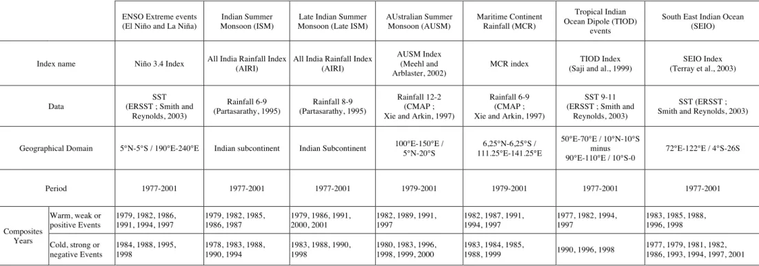
A simple method for characterizing a complex phenomenon such as the monsoon-ENSO system is to reduce it to a small number of indices. As an illustration, Meehl et al. (2003) used the time series of area-averaged precipitation for the ISM as an index for the whole TBO system. Following Webster et al. (2002) and Meehl et al. (2003), the monsoon-ENSO or TBO systems encompass the AUSM, ISM, MCR, ENSO and TIOD events. However, AUSM, ISM, ENSO and TIOD events are not always synchronized (Webster et al., 1998; Behera and Yamagata, 2003, Ashok et al., 2003). Moreover, significant precursors for anomalous AUSMs and ISMs, ENSO and TIOD events may differ considerably. In view of these considerations, major components of the monsoon-ENSO system have been identified by different indices and SST composite fields for all these different indices will be presented in this section. The different indices used in our composite analyses and the selected extreme years of theses indices are presented in Table 1.

The area-averaged SST anomaly in the eastern tropical Pacific Niño3.4 area (5°N-5°S/170°W-120°W) has been used as an ENSO index. The Niño3.4 index has been computed from the ERSST dataset. The criterion for El Niño (La Niña) years is defined by the 5-month running mean averaged Niño3.4 SST anomaly exceeding +0.5°C (-0.5°C) threshold for six

consecutive months. ENSO years determined in this way are in agreement with Trenberth (1997), except that 1997 (1998) has been added as an El Niño (La Niña) event. One purpose of this study is to identify ENSO precursors. Thus, it seems relevant to consider only the onset year of each event in computing the composites. For instance, 1991 is a well-known protracted El Niño event, and Trenberth (1997) distinguishes three onset years for it (1991, 1993 and 1994). Following the recent work of Van Loon et al. (2003), 1993 did not qualify as an El Niño event, but 1994 does. Consequently, 1991 and 1994 are retained as onset years in the present analysis. There are finally six El Niño and four La Niña (onset) years in the 1977-2001 period (Table 1).

TIOD events reach maximum amplitude during September-November (Saji et al., 1999; Saji and Yamagata, 2003). The canonical TIOD SST pattern is characterized by SST anomalies of opposite sign in the western (WTIO: 50°E-70°E/10°N-10°S) and eastern (ETIO: 90°E-110°E/10°S-0) tropical Indian Ocean during boreal fall. The WTIO and ETIO time series have also been computed from the ERSST dataset. Following Saji et al. (1999), we used the difference between WTIO and ETIO SST anomalies as a TIOD index. This time series is related to the anomalous SST gradient across the equatorial Indian Ocean. During boreal fall, the SST mean gradient across the equatorial Indian Ocean is associated with cooler SST in the west and warmer in the east. Thus, a positive TIOD index indicates a weaker or reversed equatorial SST gradient. It is interesting to note that the TIOD index is dominated by the ETIO time series during the peak season of TIOD events because the September-October-November standard deviation of ETIO SST time series (0.41) is twice the standard deviation of the WTIO SST time series (0.21). Positive (negative) TIOD events are defined in terms of September-October-November TIOD index exceeding 1 standard-deviation above (below) the mean. Using this criterion, there are four positive and three negative TIOD events in the 1977-2001 period (Table 1).

As illustrated in Terray et al. (2003a), interannual variability of ISM rainfall and dynamical indices for the traditional summer season (June-September) are strongly influenced by rainfall and circulation anomalies observed during the Late ISM (August-September). In view of these results, we computed both ISM and Late ISM composites with the help of the AIRI. Classification of weak (strong) ISM and Late ISM years are made when the standardized ISM and Late ISM indices are <-1 (>1), respectively. There are five strong and five weak ISM years, and, four strong and five weak Late ISM years during the 1977-2001 period (Table 1).

The AUSM’s relation with El Niño events has been much studied (McBride and Nicholls, 1983; Drosdowsky and Williams, 1991). Moreover, interactions between the AUSM, ISM, TIOD and ENSO have been proven many times (Webster et al., 2002; Meehl et al., 2003, Wang et al., 2003; Ashok et al., 2003). This justifies the inclusion of AUSM SST composites in this study. For this purpose, we used the time series of area-averaged precipitation for the AUSM (December-January-February, 1979-2001, 20°S-5°N, 100°-150°E) defined in previous TBO studies (Meehl and Arblaster, 2002a), and a threshold of one standard deviation. This choice leads to the definition of six strong and four weak AUSM years (Table 1).

Finally, MCR is a key factor for the monsoon-ENSO system (Terray et al., 2003b) and relationships between ENSO or TIOD events and rainfall over Indonesia have been extensively studied (Saji et al., 1999; Hendon, 2003; McBride et al., 2003). Thus, we found it relevant to compute an MCR index as the area-averaged precipitation over the domain 6°S-6°N, 111°-141°E from June to September, as used in Terray et al. (2003b). Extreme years for this MCR index are defined in a similar way as for the ISM or AUSM indices (Table 1).

The transitions of the monsoon-ENSO system in the Pacific basin occur during boreal spring in association with the so-called predictability barrier (Yasunari, 1991; Webster and Yang, 1992; Torrence and Webster, 1998). This is related to the onset time of El Niño events, which is either spring (April or May) or summer (July or August) as shown by Xu and Chan (2001). Thus, we have to examine seasons prior to the end of the austral summer (March) in order to identify common precursors that set the stage for the next phase of the monsoon-ENSO system during the following 1-yr period. In view of this, February-March seems to be a relevant starting point for the SST composite analyses based on the anomalous (Late) ISM, AUSM, MCR, ENSO and TIOD years. ISM onset occurs in May-June and TIOD events peak during boreal fall. Consequently, February-March SST anomalies will provide information on what happens, respectively, three to seven months before anomalous (Late) ISMs and TIOD events. The AUSM index is computed for December-January-February and our February-March SST composite fields for this index will give information on what happened one year before anomalous AUSMs. The February-March standardized SST composite fields over the Indian and Pacific oceans for the anomalous MCR, AUSM, ISM, Late ISM, ENSO and TIOD years are presented in Figures 1, 2 and 3. Gridpoint tests with a 90% confidence level have also been performed on all fields and are shown by shading in Figures 1, 2 and 3.

For February-March prior to El Niño (La Niña) events, there are anomalously cold (warm) SSTs in the equatorial central and eastern Pacific and a residual warm (cold) horseshoe pattern over the west and extra-tropical Pacific Ocean (Figs. 1a,b). These findings verify that February-March season is just before the growth of ENSO events in the Pacific as anticipated above. The merit of using six indices associated with the whole monsoon-ENSO system is to identify the common precursors for the various components of such complex phenomenon without making any a priori assumption about the degree of dependence of these various components. As an illustration, a significant feature is observable on almost all SST composite fields of Figures 1, 2 and 3. Cooler (warmer) SSTs in the southeast Indian Ocean and warmer (cooler) SSTs in the southwest Indian Ocean are significant precursors for weak (strong) ISMs, Late ISMs, AUSMs, MCRs, El Niño (La Niña) and positive (negative) TIOD events. Of course, there is a certain amount of variability in both the location and amplitude of the warm and cool poles for each of the composite analyses, but this SST dipole pattern is reminiscent of the subtropical SST dipole events identified by Drosdowsky (1993) and, Behera and Yamagata (2001). A closer inspection of the composite fields indicates that the pole located in the SEIO off western Australia is by far the most important both in terms of statistical significance and spatial extent. We can delimit a geographical domain 72°-122°E, 4°S-26°S, which shows up on almost all the composite maps. This domain is indicated by a black frame in Figure 3d. Consequently, we computed a February-March SST anomalies time series area-averaged over this domain in order to obtain a SST SEIO index (Fig. 4). It is noteworthy that the wavelet analysis of the SEIO index shows significant spectral peaks at TBO time scale both before and after the 1976-1977 climatic shift. Longer time scales (4-8 years) are also detected in this time series suggesting ENSO variability. Interestingly, the wavelet spectrum also suggests a continuous shortening of the period of this ENSO oscillation from 1965 till the end of the record in a such a way that TBO and ENSO periodicities are virtually indistinguishable during the last decade (Fig. 4). Thus, this wavelet analysis supports the results of the previous composite analyses in suggesting that February-March SEIO SSTs are an integral part of the TBO system.

Figure 2 corroborates the previous work by Terray et al. (2003a), who demonstrated that there are statistical relationships between SEIO SST variability in boreal winter (associated with subtropical SST dipole events) and anomalous (Late) ISMs. However, their results were derived from the 1948-1998 period and they did not discuss the impact of the 1976-1977

climatic shift on the SEIO-ISM relationship. Thus, it is worth mentioning that both ISM and Late ISM indices still have a strong and significant relationship with SEIO SSTs during the 1977-2001 time interval. This remarkable feature demonstrates the sensitivity of the ISM circulation and rainfall over India to SEIO SST anomalies. Furthermore, Terray et al. (2003a) pointed out that the Late ISM is more affected by the anomalous state of ENSO in the previous winter than the ISM as a whole, particularly for the strong monsoons. This seems to be also true for recent decades (Fig. 2).

Surprisingly, no other common SST precursors show up on the (Late) ISM, AUSM, MCR, ENSO and TIOD SST composites. Some areas exhibit more significant anomalies in a particular composite analysis, but they do not occur in all cases. For example, strong anomalies are found in the Bay of Bengal in February-March before strong Late ISMs (Fig. 2d) or negative TIOD events (Fig. 1d), but they do not emerge on La Niña or strong MCRs events (Figs. 1b and 3d). Interestingly, SST anomalies in the Pacific Ocean are much weaker. Figure 1 suggests two other SST dipole anomalies in the north and south subtropical Pacific as precursors of ENSO events. However, these SST dipole anomalies are absent on TIOD or ISM SST composites. Moreover, these SST dipole anomalies are only marginally significant compared to SEIO SST anomalies on both the El Niño and La Niña SST composites. Thus, SEIO is not always the strongest precursor area for each phenomenon taken separately, but is the best one for the whole ENSO-monsoon system.

The obvious question that then arises is the following. Why and how may the whole ENSO-monsoon system be sensitive to SST forcing in the SEIO during boreal winter, in such way that anomalous ISMs, AUSMs, MCRs, TIOD and ENSO events are all preceded by SST variability over the southern Indian Ocean? Additionally, our statistical tests suggest that this SEIO SST forcing is robust and represents the most important precursor of the monsoon-ENSO system in the whole Indo-Pacific SST forcing field, just before the growth of monsoon-ENSO events. Particular attention is focused on this SEIO SST forcing in the next section.

4. Composite analysis of cold and warm SEIO SST years

In this section, we examine the evolution of atmospheric and SST anomaly patterns associated with cold and warm SEIO SSTs during boreal winter. Given that southern Indian Ocean dipole events reach a maximum in February-March and are phase-locked to the annual

cycle (Behera and Yamagata, 2001), we again use a composite analysis for this purpose. The cold and warm extreme values of the February-March SST SEIO index (above or below a 0.5 standard-deviation threshold; full details in Table 1) were used to generate bimonthly SST, wind (850 and 200 hPa), SLP, omega (500 and 300 hPa) and latent heat flux composite fields for the following 1-yr period during the 1977-2001 time interval (Figs. 5-10). The wind composite maps shown in Figures 6, 7 and 10 are masked to exhibit only wind anomalies that exceed the 90% confidence level. Finally, it is worth mentioning that the results of this composite analysis are robust against a strengthening of the threshold or the exclusion of the exceptional 1997 El Niño event from the cold SEIO SST years.

a. Cold SEIO SST years

First focusing on cold SEIO SST composites, we observe in February-March an anomalous subtropical SST gradient (or dipole mode) in the southern Indian Ocean with cool water in the east and warm in the west (Fig. 5a). Cold SST anomalies cover a large area in the eastern Indian Ocean extending southward off Australia (reaching 45°S), northward into the Bay of Bengal and westward in the vicinity of New Guinea and the Maritime Continent. Significant warm anomalies are also found southeast of Madagascar. It is of interest that the response in the southwest Indian Ocean to the cold SEIO SST anomaly is of opposite sign although of smaller amplitude. This provides evidence of the physical nature of the SST dipole pattern in the southern Indian Ocean during austral summer. The February-March surface wind and omega anomalies patterns for the cold SEIO SST years show large and significant anomalies in the central south Indian Ocean (Fig. 6a). These anomalous patterns suggest that the Mascarene high is enhanced during February-March. Moreover, this anticyclonic anomaly is also observed at higher levels (Fig. 7a). Southeast of this anticyclonic anomaly, the total surface wind speed increases as the February-March mean 850 hPa wind is southeasterly off Australia, thereby increasing evaporation and vertical mixing. The anomalous anticyclone also reduces the cloud cover and increases the downward solar radiation to the west. In other words, this suggests that positive SST dipole events arise out of surface wind forcing via changes in latent heat flux, upper ocean mixing and Ekman transport (Behera and Yamagata, 2001). Negative omega anomalies (anomalous ascent) are observed at 500 and 300 hPa over the Philippine Sea and the Pacific Ocean warm pool (Figs. 6a and 7a). Meanwhile, there are positive omega values (anomalous subsidence) over East Asia. The significant anomalous northerlies off the East Asian coast, the significant northwesterly wind

anomalies along the west coast of Sumatra and the westerly wind anomalies in the western equatorial Pacific at 850 hPa (Fig. 6a) are dynamically consistent with this meridional structure, as are the 200 hPa southeasterly wind anomalies linking anomalous ascent over the western Pacific to anomalous sinking over east Asia around 20°N (Fig. 7a). This is a sign of a strengthening of the local meridional circulation between East Asia and the Philippine Sea. Since the surface mean wind off the west coast of Sumatra is northwesterly during this season, the total wind speed increases in February-March of cold SEIO SST years. This may contribute to the observed cooling of SSTs in the eastern equatorial Indian Ocean essentially through enhanced evaporation and vertical mixing since the seasonal winds (northwesterlies) are downwelling favourable during this season. All these features suggest a stronger East Asian winter monsoon. Interestingly, a strong East Asian winter monsoon is one of the precursors of El Niño events identified by Xu and Chan (2001). Over the South Pacific, a cyclonic circulation and anomalous ascent are found off the eastern coast of Australia, where the South Pacific Convergence Zone (SPCZ) is normally located (Fig. 6a). Finally, it is noteworthy that the wind and SST patterns over the central and eastern equatorial Pacific sectors are not significant during February-March of cold SEIO SST years.

SST patterns during boreal spring of the cold SEIO SST years show a decay of the SST dipole pattern (Fig. 5b). However, SEIO SST anomalies tend to persist and move northeastward. This suggests that positive feedbacks between the atmosphere and ocean may allow a persistence of the SST anomaly in the SEIO area. Meanwhile, there are positive omega anomalies and an anticlockwise surface circulation over the SEIO, and negative omega values and an associated clockwise surface circulation between Madagascar and 100°E (Fig. 6b). This pattern is the signature of a delayed westward seasonal movement of the Mascarene high from boreal winter to boreal summer (Terray et al., 2003a). In order to diagnose possible air-sea feedbacks, which may allow the persistence of the cold SEIO SST anomalies during boreal spring, the SLP, latent heat flux and rainfall composites observed in April-May of the cold SEIO SST years are shown in Figure 8. For the latent heat flux composites, positive values indicate heat loss from the ocean (Fig. 8c). First, we observe that a low (high) pressure anomaly develops near the warm (cold) SST anomaly in the southern Indian Ocean by April-May (Fig. 8a). This result is consistent with what might be expected from linear quasi-geostrophic theory (Gill, 1982). That is, a low (high) pressure anomaly is generated over a warm (cool) SST forcing. Moreover, the SLP and rainfall anomaly patterns suggest that the maritime Inter Tropical Convergence Zone (ITCZ) from the North of Madagascar to

northwestern Australia-Indonesia is weakened while positive precipitation anomalies are observed in the southwest Indian Ocean. These results are consistent with the anomalous divergence (convergence) over SEIO (southwest Indian Ocean) areas in spring of positive SST dipole events (Figs. 6b and 7b). This results in an atmospheric sink over the SEIO. Now, the southeasterly wind anomalies between Sumatra and Australia associated with the anomalous subsidence over the SEIO (Fig. 6b) represent an increase in wind speed relative to climatology, as the seasonal wind changes from northwesterly to southeasterly in this region during boreal spring. This implies further cooling of SEIO SSTs via increased upper ocean mixing and evaporation (Fig. 8c). These cold SST anomalies further decrease atmospheric convection, which reinforces the atmospheric heat sink at higher levels (Fig. 7b). The most suppressed convection and negative rainfall anomalies (Fig. 8e) are located eastward of the anomalous anticyclone (Fig. 8a), suggesting that this anomalous anticyclone is partly an atmospheric response to the heat sink through descending Rossby waves to its west (Gill, 1980). This strengthens the anomalous low-level anticyclonic circulation. These processes represent a seasonally positive feedback between the wind, evaporation and SST in the SEIO (Li et al., 2003; Fischer et al. 2003). It may explain both the persistence and the northeastward shift of the cold SST anomalies there. Furthermore, Fischer et al. (2003) found, using a coupled General Circulation Model (GCM), that this positive feedback is particularly active during boreal winter and spring in the SEIO. On the other hand, the cyclonic wind anomalies over the southwestern Indian Ocean imply Ekman divergence and upwelling. These processes add to the reduced solar radiation and enhanced evaporation off the adjacent warm anomaly (associated with its positive rainfall and anomalous ascendance) to reduce the warm SST anomalies southeast of Madagascar. These processes represent a negative feedback, which may damp the warm SST anomalies in the southwest Indian Ocean (Behera and Yamagata, 2001).

By April-May, the cold SST anomalies have also spread eastward between Australia and the Maritime Continent, reaching the vicinity of New Zealand (Fig. 5b). Associated with these anomalous SSTs, positive omega anomalies also develop over eastern Australia, indicative of anomalous subsidence (Fig. 6b). Prominent southerly wind anomalies and negative rainfall anomalies prevail off the east coast of Australia (Figs. 6b and 8e). This suggests an enhancement and a northward shift of the Australian high in late boreal spring associated with an earlier onset of the Australian winter monsoon. Such a feature has already been noted by Xu and Chan (2001) as a key factor in determining the onset of El Niño events. In the equatorial western Pacific, significant 850 hPa westerly wind anomalies of about 1.5 m/s

extend now from 130°E to the date line (Fig. 6b) and significant easterly 200 hPa wind anomalies also extend eastward (Fig. 7b). This suggests that the meridional flow pattern off Australia produces a strong convergence over the western Pacific, enhancing the westerly anomalies. Finally, significant warm SST anomalies develop south of Australia and off the west coast of Chile, in association with an equatorward shift of the mid-latitude westerlies and an expanded trough in the South Pacific (Figs. 6b and 8a). These changes in the South Pacific extratropical circulation may be viewed in terms of the modulations of the western Pacific regional Hadley cell observed during cold SEIO years (Figs. 6b and 7b). Moreover, the anomalous SLP pattern in Fig. 8a represents a weakening of the SLP gradient around the South Pacific subtropical high which is consistent with a reduction of the trade winds in the south Pacific (Fig. 6b). Van Loon et al. (2003) show the importance of this expanded trough in the South Pacific for the El Niño evolution. Finally, the anomalous SLP and wind patterns at this time of the year highlight possible links between this expanded trough and a modulation of the semiannual oscillation in the South Pacific (Van Loon et al., 2003). These aspects of the SEIO SLP and wind composites need further investigations which will be reported in a future study.

In June-July, anomalous cold SSTs first seen in a large part of the Indian Ocean are now limited to the eastern Indian Ocean (Fig. 5c). This area is similar to the Sumatra area defined by Xie et al. (2002); SSTs in this area have been proven in this study to be an important trigger (with ENSO influence) of TIOD events. At the same time, warm anomalies in the southwest Indian Ocean have considerably weakened. This is consistent with the negative feedback discussed above. However, negative omega anomalies (anomalous ascent) in the central Indian Ocean between 15°S and 40°S and positive omega anomalies to the west of the cold SSTs in the eastern Indian are persistent features of the atmospheric circulation over the southern Indian Ocean and remain observable at higher levels (Figs 6c and 7c). The associated clockwise circulation in the western Indian Ocean (south of the Equator) suggests a persistent weakening of the Mascarene high during the early ISM of the cold SEIO SST years. Turning our attention now back to the SEIO, the development of significant southeasterly wind anomalies off Sumatra, collocated with the cold SSTs, are again consistent with the persistence of positive feedbacks between the anomalous anticyclone there and the cold SST anomalies to the east (Li et al., 2003, Fischer et al., 2003). In addition, a wind-thermocline-SST feedback may now reinforce the cold wind-thermocline-SST anomalies in the eastern Indian Ocean. That is, the mean surface flow changes from northwesterly downwelling-favourable winds to

southeasterly upwelling favourable winds along the Sumatra coast in early boreal summer (Fischer et al., 2003). Thus, the low-level anticyclonic anomalous flow southwest of Sumatra in June-July of the cold SEIO SST years accelerates the seasonal southeasterly winds and increases the total wind speed. These anticyclonic surface wind anomalies have an upwelling component along the Sumatra coast and an anomalous easterly component along the equatorial wave guide (Fig. 6c). These factors may contribute to the persistence of the cold SST anomalies off Sumatra as well as the propagation of these anomalies across the equatorial eastern Indian Ocean through upwelling (Fig. 5c). Again, these cold SST anomalies reduce atmospheric convection and rainfall as suggested by the positive omega anomalies (anomalous subsidence) at both 500 and 300 hPa between Australia and Sumatra in Figures 6c and 7c. This further enhances the mean southeasterly flow off Sumatra that, in turn, reinforces the underlying cold SSTs. According to the coupled GCM results of Fischer et al. (2003), the wind-thermocline-SST feedback is more important than the wind-evaporation-SST feedback off the west coast of Sumatra during boreal summer.

In June-July, cold SST anomalies also spread westward into the Pacific Ocean warm pool and southeastward in the south Pacific (Fig. 5c). At the same time, we observe the emergence of significant warm SST anomalies in the central equatorial Pacific. These are connected to the enhanced and persistent warm SST anomalies in the southeast Pacific. Highly significant warm SST anomalies are also found southeast of New Zealand. This Pacific SST anomaly pattern displays evident El Niño features with development of warm SST anomalies in the eastern Pacific and formation of the south branch of the traditional cold horseshoe pattern in the western Pacific (Harrison and Larkin, 1998). In agreement with these SST anomalies, the anomalous wind and omega patterns show anomalous ascent over the central Pacific and a significant weakening of the east-west circulation over the western Pacific (Figs. 6c and 7c). Anomalous subsidence is now found over the Maritime Continent, dynamically consistent with the easterly wind anomalies over the eastern equatorial Indian Ocean and the westerly anomalies over the western Pacific (Fig. 6c). The suppressed convection over the Maritime continent may also reinforce the anomalous SEIO anticyclone via descending Rossby waves to the southwest of this atmospheric heat sink (Wang et al., 2003). The anomalous flow pattern off Australia is similar to April-May with prominent southeasterlies stretching from New Zealand to the Maritime Continent. This may contribute toward the development and eastward propagation of the westerly wind anomalies over the equatorial Pacific.

In August-September, there are positive omega values (anomalous subsidence) over the Indian subcontinent suggesting a weak Late ISM. The SLP composites (not shown) show a

tilted band of high SLP anomalies stretching from northwestern Australia to the North Arabian Sea. The more significant SLP anomalies are located to the southwest of Sumatra, consistent with the positive feedbacks discussed above. The anomalous circulation pattern suggests a significant weakening of the low-level circulation, as indicated by a reduced Somali Jet and the significant clockwise circulation anomalies apparent around Madagascar (Fig. 6d). At 200 hPa, we also observe that both the Tibetan Plateau and Mascarene highs are weakened and shifted eastward during cold SEIO SST years (Fig. 7d). In other words, the whole late ISM circulation is anomalously reduced during cold SEIO SST years. The weaker surface monsoon circulation will influence the Indian Ocean SST variability since wind anomalies are observed in regions where major upwelling occurs (Xie et al., 2002). In the western Indian Ocean, the reduced monsoon flow is accompanied by weaker wind mixing, less evaporation, but also decreasing upwelling along the east Africa coast and south of the Equator (Xie et al., 2002; Webster et al., 2002; Loschnigg et al., 2003). Meanwhile, the weaker ISM induces a stronger interhemispheric gradient in the eastern Indian Ocean with a stronger interhemispheric flow into the Bay of Bengal (Terray et al., 2003a). Even though these wind anomalies are not significant in our composites (Fig. 6d), they do exist (not shown). Thus, the persistent offshore flow near Sumatra will enhance equatorial and coastal upwelling. It may contribute to the northwestward propagation and the amplification of the cold SST anomalies in the eastern Indian Ocean from June-July to August-September (Fig. 5d). In summary, the anomalously weak monsoon winds observed during the late ISM of the cold SEIO SST years will favour warmer water in the western Indian Ocean and colder water in the eastern Indian Ocean. The induced perturbation of the SST gradient across the equatorial Indian Ocean adds to the cold SEIO SSTs, and may then trigger a TIOD event in the following fall (Figs. 5e and 6e) as suggested by Webster et al. (2002).

Significant positive (downward) omega anomalies over the Maritime Continent and negative (upward) omega anomalies in the central Pacific near the date line are observed by August-September (Fig. 6d). The anomalous atmospheric pattern off Australia, characterized by strong southerly wind anomalies, persists. Furthermore, strong northerly wind anomalies now prevail over the Philippine Sea in association with the growth of the west Pacific anomalous anticyclone (Wang et al., 2003). Thus, these two anomalous meridional circulations produce a stronger anomalous convergence over the western equatorial Pacific, which enhances both the westerly anomalies and their eastward propagation over the equatorial Pacific (Fig. 6d). Consistent with this scenario, the 850 and 200 hPa Pacific wind anomaly patterns show the dramatic perturbation of the Walker circulation associated with El

Niño events. This suggests the SEIO area in boreal winter, as a key precursor of the ENSO evolution in the Pacific, since all these features emerge progressively during cold SEIO SST years.

In October-November, the SST composite depicts the appearance of a TIOD event with an anomalous SST gradient and strong easterly wind anomalies across the equatorial Indian Ocean (Figs. 5e and 6e). This pattern resembles the canonical TIOD event described in Saji and Yamagata (2003, their Fig. 2). Cold SST anomalies are observed south of the equator trapped to the west coast of Indonesia, and a tilted band of positive SST anomalies are seen stretching from the North Arabian Sea to the SEIO. Interestingly, the warm SST anomalies in the western equatorial Indian Ocean are not significant, and the most significant warm SST anomalies are located north and south of the equator. This anomalous SST pattern in the Indian Ocean seems related to the changes in the Late ISM wind pattern described above, still present over the southwestern part of the basin in October-November of the cold SEIO SST years (Fig. 6e). Thus, the anomalous SST pattern caused by the anomalous Late ISM flow seems to trigger the coupled ocean-atmosphere instabilities governing the evolution of a TIOD event (Webster et al., 1999). However, it is noteworthy that this canonical TIOD evolution occurs in association with cold SEIO SST anomalies six months before. This confirms earlier work by Drosdowsky (1993), which showed that SEIO SSTs in late boreal winter is a good precursor of TIOD events. Over the Pacific Ocean, the El Niño pattern is now fully developed with a weakened Walker cell (Figs. 6e and 7e). The eastward propagation of the equatorial westerly wind anomalies continues, now reaching 100°W. The whole central and eastern equatorial Pacific Ocean is now covered by significant positive rainfall anomalies (not shown), dynamically consistent with the negative omega anomalies observed in these areas (Fig. 6e). The anomalous flow pattern off the east coast of Australia fades away.

In December-January of the following year, the strong signature of the TIOD event evident in October-November dies away (Fig. 5f). The easterly surface wind anomalies along the equatorial Indian Ocean propagate eastward in association with the southeastward seasonal migration of the convective maximum in Indo-Pacific areas (Fig. 6f; Meehl et al., 2003). This evolution is mainly due to the fact that the above-described positive feedbacks switch their sign after boreal fall. After November, the background flows reverse direction over the eastern Indian Ocean. Thus, both the wind-evaporation-SST and wind-thermocline-SST

feedbacks switch their polarity when the winter monsoon prevails. Anomalously cold SSTs are found south of Madagascar, whereas warm SST anomalies now cover the whole tropical Indian Ocean (Fig. 5f). The anomaly SST pattern observed over the Indian Ocean in December-January is very similar to the one noted in February-March, but with opposite sign and weaker amplitude. This indicates the strong TBO tendency of SEIO SST variability (Fig. 4). The 850 hPa anomalous wind pattern in the southern Indian Ocean is also reversed compared to February-March, and is dynamically consistent with a weaker Mascarene high in austral summer (Fig. 6f). The associated northwesterly wind anomalies off the west coast of Australia may contribute to the reinforcement of the reversed SST dipole pattern for the following year. In the Pacific, the El Niño pattern has now evolved to its mature phase (Fig. 5f). The whole equatorial Pacific is now covered with westerly surface wind anomalies (Fig. 6f). Finally, a remarkable teleconnection Pacific-North American pattern emanating from the central Pacific crosses the North Pacific and extends to North America in the form of a pronounced wave train pattern at both 850 and 200 hPa levels. This result is not a surprise, as the El Niño related SST anomalous pattern in Figure 5f is known to excite the Pacific-North American pattern during boreal winter (Wallace and Gutzler, 1981). However, the fact that this pattern shows up in SEIO SST composites stresses again the significance of SEIO SST anomalies in the phase transitions of the monsoon-ENSO system.

b. Warm SEIO SST years

It is of interest that the response of the monsoon-ENSO system to warm SEIO SST anomalies in February-March is of opposite sign although of smaller amplitude during the following 1-yr period (Figs. 9 and 10). By February-March, we observe the occurrence of a negative dipole event in the southern Indian Ocean and a weakening of the East Asian winter monsoon associated with the west Pacific anomalous anticyclone (Wang et al., 2003). From April-May to August-September, significant northerlies persist off the east coast of Australia. During boreal summer, the Maritime Continent and the eastern Indian Ocean are regions of enhanced convection. The SST and atmospheric composites show a La Niña evolution with the emergence of cold SST anomalies in the central equatorial Pacific and easterly surface wind anomalies over the western Pacific and Maritime Continent in June-July (Figs. 9 and 10). The traditional horseshoe pattern also emerges progressively. The Late ISM is stronger than normal during warm SEIO SST years, with a significant enhancement of the interhemispheric ISM circulation from August-September to October-November (Figs. 10de),

inducing cold SST anomalies in the western Indian Ocean through enhanced evaporation, ocean mixing and upwelling (Fig. 9d). This contributes to the establishment of a negative TIOD event with warm SST anomalies in eastern Equatorial Indian Ocean and cold ones in the west during boreal fall (Fig. 9e). While TIOD variability is evident in warm SEIO SST composites, it has a much lesser significance than in cold composites, with SST anomalies over the equatorial Indian Ocean not significant at the 10% confidence level in October-November of the warm SEIO SST years (Fig. 9e).

Thus, similar patterns with reversed polarity are observable, but of course some discrepancies exist. The most striking one occurs in February-March when warm SST anomalies spread over the whole north Indian Ocean and the China Sea (Fig. 9a). A close inspection of the SST, wind and omega composites in February-March of the warm SEIO SST years shows the signature of a negative dipole event in the southern Indian Ocean as might be expected, but also the decay phase of an El Niño event in the Pacific (Figs. 9a and 10a). This is illustrated by significant warm SSTs in the eastern equatorial Pacific and westerly wind anomalies south of the equator in the central Pacific during February-March. Moreover, the association of warm SSTs in the Pacific with warm SSTs in the tropical Indian Ocean during boreal winter (Fig. 9a) has been well documented in the context of El Niño events. This may contribute to the much larger extent of significant warm anomalies observed over the Indian Ocean during February-March of warm SEIO SST years relative to cold ones in cold SEIO SST years (Fig. 5a). However, this feature is not evident by studying selected years for El Niño and warm SEIO SST events (Table 1): only two El Niño years, 1982 and 1997, are followed by warm SEIO SST years (1983 and 1998). Moreover, two La Niña years (1984 and 1995) are also followed by warm SEIO SST years (1985 and 1996). In other words, the greater spatial extent of the warm SST anomalies are certainly attributable to the exceptional strength of both the 1982 and 1997 El Niño events, but negative SST dipole events in the southern Indian Ocean are not necessarily preceded by an El Niño year. This suggests that others factors than ENSO may be responsible for the occurrence of SST dipole events in the south Indian Ocean during austral summer. In this respect, the possible link between the Mascarene high pulses and the variability of the midlatitude circulation in the southern hemisphere needs further investigation and could be an important contributing factor (Fauchereau et al. 2003).

The SEIO SST anomaly in boreal winter has been identified as a precursor to El Niño or the TIOD, with a lead of several months. In this section, we assess its predictive skill through a correlation analysis. We also compare the results with other well-known ENSO precursors.

In accordance with theoretical and observational studies (Jin, 1997; Meinen and McPhaden, 2000), the upper ocean equatorial heat content in the Pacific is a useful ENSO precursor which successfully predicts through the ENSO spring persistence barrier (Clarke and Van Gorder, 2003). This useful property may be explained by the fact that the upper ocean equatorial heat content takes into account the interannual state of the Pacific Ocean (Wyrtki, 1985; Meinen and McPhaden, 2000). As noted in SEIO SST composites, the zonal wind stress anomaly in the far-western equatorial Pacific is another crucial parameter in ENSO evolution (Barnett, 1983; Gutzler and Harrison, 1987). This feature is also somewhat discernable in ENSO composites (Clarke and Van Gorder, 2001, 2003; Xu and Chan, 2001; Wang and Zhang, 2002). As for the upper ocean equatorial heat content, the far-western Pacific zonal equatorial wind stress anomaly leads ENSO events by several months and can predict through the ENSO spring persistence barrier. Based on the precursor properties of Niño3.4 SST, upper ocean equatorial heat content and far-western Pacific zonal equatorial wind stress anomalies, Clarke and Van Gorder (2003) constructed a linear regression model to predict Niño3.4 SST for various leads and showed that this simple model performs at least as well as other ENSO prediction models. To put the results of our analysis in perspective, we first compare the lead correlations of SEIO SST anomalies and these various ENSO precursors with Niño3.4 SST for various leads up to 12 months.

Following Clarke and Van Gorder (2003), we define the upper ocean equatorial heat content as the monthly mean 20°C thermocline depth anomaly (Z20 hereafter) averaged over the equatorial Pacific (5°S-5°N, 130°E-80°W). This time series is computed from the SODA dataset. We define the western equatorial Pacific zonal wind anomaly (WPAC hereafter) to be the zonal 850 hPa wind anomaly area-average over the region 130-160°E, 5°S-5°N as suggested by Clarke and Van Gorder (2001, 2003). Figure 11 shows the lag-correlations between Niño3.4 and SEIO in each month and Niño3.4, SEIO, Z20 and WPAC in the preceding winter (February-March). We obtain similar results with other SST indices such as Niño3 or Niño4 or if we define WPAC and Z20 from ENSO composites (not shown). In order to facilitate the comparison between the various ENSO precursors, we also plotted the 95% confidence levels assuming 25 degrees of freedom and the opposite values of the correlations between SEIO and Niño3.4 in Figure 11. As an illustration, we have a correlation of +0.45

between SEIO in February-March and Niño3.4 in January, but this correlation is indicated as –0.45 in Figure 11. We first observe that the auto-correlation of Niño3.4 SSTs dies away in July and is near zero after September. This sharp decrease in persistence in the boreal spring of ENSO indices is a result of the phase locking of ENSO to the annual cycle, which tends to cause transitions in ENSO indices to occur during boreal spring (Webster and Yang, 1992; Torrence and Webster, 1998). On the other hand, SEIO persistence remains significantly high until October. This is linked to the fact that these SST anomalies strongly depend on the seasonal evolution of the wind field over the Indian Ocean as described in the previous section. The transition for SEIO SST anomalies occurs in late fall or early boreal winter when the seasonal wind over the eastern Indian Ocean turns from southeasterly to northwesterly. After this reversal of the mean wind, the local air-sea feedbacks in the SEIO change from positive to negative. The easterly wind anomalies do not accelerate but rather decelerate the seasonal wind, which becomes downwelling-favourable along the west coast of Sumatra. This may explain why SEIO auto-correlations decrease rapidly and even change sign from October to December.

Turning now our attention to the prediction of Niño3.4 evolution, we observe that the various ENSO precursors have different relationships with the Niño3.4 monthly time series. Consistent with past studies, the lag-correlation analysis shows that both WPAC and Z20 are significantly related to the occurrence of an El Niño event. WPAC in February-March is positively correlated with Niño3.4 from January to December and the correlation coefficients increase from 0.32 in April to 0.63 in December. The correlations between Z20 and Niño3.4 switch sign in April, then increase rapidly from April to July and slowly from July to December. The highest correlation between Z20 and Niño3.4 is observed in December and is as high as 0.70. Finally, we observe that the correlations between February-March SEIO and monthly Niño3.4 are positive and significant until March, reverse abruptly their sign from April to June as for Z20 and decrease steadily from July to October. From October to December, the correlations between SEIO and Niño3.4 are around -0.70 and -0.75. Moreover, from August to December, the SEIO index gives consistently better results than WPAC or Z20. This period basically concerns the growth and peak of El Niño events (Larkin and Harrison, 2002), thus confirming the significance of SEIO SST anomalies as a precursor to ENSO events. Moreover, the fact that the correlations between SEIO and Niño3.4 evolve from positive and significant in late boreal winter to negative and highly significant in the next boreal winter reinforces the suggestion that Indian Ocean SST anomalies, and

particularly SEIO ones, play a primordial role in the ENSO transitions during recent decades (Yu et al., 2003).

To further compare the predictive skill associated with SEIO SST anomalies and other ENSO precursors, the lag-correlations between Z20, WPAC, and SEIO in each month and Niño3.4 in October-December are shown in Figure 12. We also present in this figure the correlations with a meridional 850 hPa wind time series off the East coast of AUStralia (EAUS hereafter). Inclusion of this wind index is motivated by the results presented in Section 4 and the work of Xu and Chan (2001). This time series is defined as the area-averaged meridional 850 hPa wind anomaly over the region 150-175°E, 15-40°S from ENSO composites (not shown). As in Figure 11, opposite values of correlation between SEIO and Niño3.4 are plotted in Figure 12. Figure 12 suggests that SEIO SST anomalies perform at least as well as other well-established ENSO predictors before boreal spring. Correlation between SEIO SSTs in February and Niño3.4 in October-December is as high as -0.74, and SEIO performs better than other predictors for this time lead. This highlights the importance of SST dipole events, highly phase locked with the seasonal cycle, for the emergence of SEIO SST anomalies. Interestingly, significant correlations between WPAC and Niño3.4 occur abruptly in March-April, which is about one to two months after the emergence of SEIO SST anomalies, while the correlations with Z20 remain stable around these months. During boreal summer and fall, WPAC outperforms other indices with maximum correlations around 0.82 in August-September. This suggests that a persistent wind forcing or a collection of anomalous wind forcing events over the far western equatorial Pacific from boreal spring to late boreal summer associated with the eastward shift of the Pacific Walker cell is an important contributory factor in ENSO evolution.

Since the importance of the various ENSO predictors varies with season and SEIO SSTs are among the best ones before boreal spring, it is interesting to investigate relationships between SEIO SSTs in February-March and other ENSO precursors. However, we restrict this analysis to monthly WPAC time series, as the ocean heat content in the equatorial Pacific is an intrinsic quantity of the ENSO process and is not directly related to SEIO SST anomalies, as suggested above. The lag-correlations of SEIO and WPAC (at both 850 and 200 hPa) in February-March with monthly 850 and 200 hPa WPAC time series are shown in Figure 13. SEIO in February-March is a better predictor of the evolution of the Pacific Walker cell during summer and fall than the WPAC indices themselves. Interestingly, the correlations with the monthly 200 hPa WPAC index are roughly the opposite of those with the monthly 850 hPa WPAC index from May to December. This suggests that the evolution of the Pacific

Walker cell has a close relationship with SEIO SST anomalies during late winter. Obviously, SEIO SST anomalies may play an important role in triggering persistent surface wind anomalies over the Pacific warm pool during the growth of El Niño events, via anomalous subsidence over the Maritime Continent, anomalous ascendance over the west Pacific and anomalous southerlies off the northeast coast of Australia associated with the persistent anomalous SEIO anticyclone.

SEIO has also been identified as a possible precursor for TIOD events in boreal fall. In order to confirm this feature, a similar lag-correlation analysis between SEIO SSTs in February-March and various monthly TIOD indices has been undertaken. In addition to SST ETIO, WTIO and TIOD indices defined in Section 3, we also included in this analysis the zonal 850 hPa wind anomaly over the equatorial Indian Ocean (5°S-5°N, 70°-90°E, Ueq hereafter) in order to clearly identify the coupled air-sea TIOD pattern over the tropical Indian Ocean. The results presented in Figure 14 appear to be consistent with those of Sections 3 and 4. For instance, SEIO SSTs in February-March are significantly and positively correlated with ETIO SSTs from January to November. The correlations increase from August to October, suggesting the existence of a positive feedback during these months, and rapidly fade away afterwards. Similarly, correlations with WTIO SSTs are highly positive during boreal winter, but reverse their sign during boreal summer to become significantly negative in November. In other words, these lag-correlations reproduce the phase lag in the SST anomaly evolution between ETIO and WTIO, which characterizes TIOD events (Saji and Yamagata, 2003). Finally, the correlations with TIOD and Ueq indices are highest and significant during October and November, suggesting that SEIO SST anomalies in February-March may trigger the coupled air-sea instability inherent in TIOD events. Together, these results suggest that subtropical Indian Ocean SST anomalies in February-March are also a significant precursor of TIOD indices during fall, the peak season of TIOD events.

SEIO has also been suggested as a significant precursor for the variability of the various monsoon systems in the Indo-Pacific region. Table 2 lists the correlation coefficients of SEIO SSTs in February-March with rainfall and dynamical indices for the Indian and Australian monsoon systems during the following boreal summer, fall and winter. In addition to the AIRI, MCR, and Australian monsoon indices, we have included the ISM dynamical indices proposed by Wang and Fan (1999) and Wang et al. (2001). Based on empirical relationships between convection and vertical shear anomalies, they proposed that the ISM system may be represented by a Westerly Shear Index (WSI1), a Southerly Shear Index (SSI1) and the

difference of the zonal wind anomalies (DU1) between a southern region and a northern region. The precise definition of these indices is given in the caption of Table 2.

For the Early ISM (June-July), the correlations of the rainfall and dynamical ISM indices with SEIO SSTs in February-March are all negligibly small. However, these correlation coefficients become positive and significant at least at the 99% confidence level for the Late ISM. This corroborates the fact that SEIO SST variability is essentially linked to the Late ISM even though this feature is not well understood (Terray et al., 2003a). Interestingly, the highest correlation is observed for SSI1 (0.66), which is related to the cross-equatorial flow off the African coast and the local Hadley circulation. This is consistent with the existence of positive air-sea feedbacks in the SEIO during late summer (Terray et al., 2003a). It is interesting to observe that warm SEIO SST anomalies in February-March are followed by positive and significant rainfall anomalies over the Maritime Continent and North Australia from early summer to winter (Table 2). Once again, the coefficients are particularly high during August-September. This implies that SEIO SSTs are linked to both the winter and summer Australian monsoons in addition to the Maritime Continent heat source. This is in agreement with the composite analysis of Section 4.

6. Summary and discussion

Because the SST signal in the Pacific Ocean precedes that in the Indian Ocean during boreal fall and winter, the possibility that the Indian Ocean plays a role in ENSO evolution has been largely overlooked in the past. Since the late 1970s, the evolution of ENSO events and the relationships between the ISM and ENSO have significantly changed. The purpose, therefore, of this paper is to statistically re-examine, the relationship between Indian Ocean SSTs and the whole monsoon-ENSO system, noting especially the changes that have taken place after 1976.

a. Observational results

Composite analyses of SST fields with respect to ENSO, (Late) ISM, AUSM, MCR, and TIOD indices reveal that southern Indian Ocean SST dipole events during boreal winter are the unique common SST precursor of these various phenomena before the growth of ENSO events in boreal spring. SEIO SST anomalies induced by such dipole events are highly persistent. This reinforces the idea that Indian Ocean SST anomalies, and particularly those in