HAL Id: hal-00653756
https://hal.inria.fr/hal-00653756v2
Submitted on 20 Dec 2012
HAL is a multi-disciplinary open access
archive for the deposit and dissemination of
sci-entific research documents, whether they are
pub-lished or not. The documents may come from
L’archive ouverte pluridisciplinaire HAL, est
destinée au dépôt et à la diffusion de documents
scientifiques de niveau recherche, publiés ou non,
émanant des établissements d’enseignement et de
Budan Tables of Real Univariate Polynomials
André Galligo
To cite this version:
André Galligo. Budan Tables of Real Univariate Polynomials. Journal of Symbolic Computation,
Elsevier, 2013, 53, pp.64-80. �10.1016/j.jsc.2012.11.004�. �hal-00653756v2�
Budan Tables of Real Univariate Polynomials
Andr´
e Galligo
Laboratoire de Math´ematiques Universit´e de Nice-Sophia Antipolis Parc Valrose, 06108 Nice (France).
Abstract
The Budan table of f collects the signs of the iterated derivatives of f . We revisit the classical Budan-Fourier theorem for a univariate real polynomial f and establish a new connectivity prop-erty of its Budan table. We use this propprop-erty to characterize the virtual roots of f (introduced by Gonzalez-Vega, Lombardi, Mah´e in 1998); they are continuous functions of the coefficients of f. We also consider a property (P) of a polynomial f , which is generically satisfied, it eases the topological-combinatorial description and study of Budan tables. A natural extension of the in-formation collected by the virtual roots provides alternative representations of (P)-polynomials; while an attached tree structure allows a finite stratification of the space of polynomials with fixed degree.
Key words: Budan-Fourier theorem; virtual roots; roots of real univariate polynomial; Budan
table; genericity; representation of univariate polynomials; Hermite-Birkhoff interpolation; B-tree; stratification; incidence relations.
1. Introduction
Counting and localizing roots of univariate polynomials is a basic task in Algebra and Numerical analysis. Many known techniques and interesting historical notes can be found e.g. in the book (24) of Rahman and Schmeisser. Established two centuries ago the Budan-Fourier theorem connects the number of real roots of a polynomial in an interval with the sign variations of a sequence and inspired the invention of Sturm sequences. It also gave rise to efficient and certified subdivision algorithms see (7) and (1).
Subdivision methods exploit the ordered structure of the real numbers, and are widely applied for calculating good approximations of solutions of polynomial equations or in-tersections of surfaces in many applied sciences. The analysis of their complexity and
Email address: [email protected]( Andr´e Galligo).
efficiency relies on the the geometric and algebraic nature of the inputs. The dictionary between invariants readable on equations and features of varieties, in complex algebraic geometry, is ultimately based on the fact that a polynomial of degree n admits n roots. This is not the case for real roots. A natural strategy for studying properties of real alge-braic varieties is to consider simultaneously roots of iterated derivatives of the input. A progress was achieved by Gonzalez-Vega, Lombardi, Mah´e in (11) when they introduced the concept of the n virtual roots of a degree n polynomial f (which depend continu-ously on the coefficients of f ), to provide a good substitute to its n complex roots. Their motivation was an attempt to prove Pierce-Birkhoff conjecture on the representation of C0-polynomial spline functions. Virtual roots were then studied by Coste, Lajous,
Lom-bardi, Roy in (9), and recently by Bemb´e in his PhD thesis (5).
The table containing the signs of all the derivatives of a polynomial f is called, in this paper, Budan table. The table is an infinite rectangle contained in the real plane, formed by positive and negative rectangular blocks, separated by segments corresponding to roots of derivatives. This structure was used by various mathematicians for separating and labeling the different real roots of a polynomial, see (7). However up to now, authors considered properties of either rows or columns of a table, or their sign variations but not the table “itself”. Here, we adopt a 2D point of view, re-interpret known results and present new ones. We analyze the different admissible configurations of successive rows in such a table and deduce the 2D same-sign-connectivity of the positive (resp. negative) blocks components, then characterize the virtual roots using this data.
We define a simple property, we call (P), on the roots of the iterative derivatives of a monic polynomial f , which is generically satisfied. Then, for a (P)-polynomial, i.e. assum-ing (P), we study and characterize the topological and combinatorial properties of the corresponding Budan table and virtual roots. We specialize results of Hermite-Birkhoff interpolation (see e.g. (21)) to our setting, to better analyze the relation between a (P)-polynomial f and its virtual roots. We also introduce a finite discrete invariant, the B-tree of a (P)-polynomial f ; and initiate the study of the attached stratification by semi-algebraic sets of the space of (P)-polynomials. Then we extend most of the results to the general case when (P) is not necessarily satisfied.
The same-sign-connected components of the Budan table can be interpreted as plane surfaces delimited by discretized curves which can be approximated by continuous ones. This point of view was initiated in (6) and in (12) using derivatives with non-integer orders, called fractional derivatives. We plan to develop it further in a future work (13).
The paper is organized as follows. Section 2 provides basic definitions and properties presented with our point of view. Section 3 introduces our generic assumption (P), then presents our results in this generic case and define our new invariant the B-tree; they are illustrated with simple examples; the proofs are collected in Section 4. Section 5 exam-ines admissible configurations for Budan tables and other invariants in the non generic case and establishes continuity results. Section 6 concludes with some extensions and potential applications.
A partial and preliminary version of our approach was presented in the first part of our talk at the ISSAC’2011 conference, (and in the corresponding proceeding paper (6)).
Acknowledgements
We thank D. Bemb´e for his collaboration in the preparation of our joint proceeding paper (6). He has now other interests and did not participate to the elaboration of the present work. We also thank the anonymous referees for their careful reading of a previous version of this paper and their suggestions. The author was partially supported by the European ITN Marie Curie network SAGA.
Notations:
We denote by R the field of real numbers, by R[x] the ring of real univariate polynomial, by R[x]n the corresponding vector space when the degree is at most n; it is equipped
with the L2 norm on the coefficients in the monomial basis. We denote by f a monic
polynomial of degree n, f := xn+Pi=n−1
i=0 aixi, the set of coefficients (ai) belongs to Rn.
The affine space En of monic polynomials of degree n is identified with Rn.
For an integer m, we denote by f(m) the m−th derivative of f , with f(0):= f .
2. Basics on Budan tables
In this section, after the definition of a Budan table, we list classical results around Budan-Fourier theorem, the proofs are elementary and can be found e.g. in (24) chapter 10, section 1. We also recall results of (11; 9).
The simplest observation that we will exploit in our approach is the following elemen-tary lemma.
Lemma 1. Assume that a is a root of f , then in a small enough interval ]a, a + h[, h > 0, f and its derivative f′
have the same sign.
Proof. Express f (x) as a definite integral of f′
(x) on a small interval ]a, a + h[ where f′
keeps the same sign. 2
Definition 2. Let f be a monic univariate polynomial of degree n. The Budan table of f is a subset of the real plane equal to the union of n + 1 infinite rectangles of height one Li:= R × [i − 1/2, i + 1/2[ for i from 0 to n, called rows.
For i from 0 to n, each row Liis the union of a set of open rectangles (infinite on the left
and right sides of the row) having the property that the sign of the (n−i)−th derivative of f is constant on each of them, they are separated by vertical segments, corresponding to roots of this derivative. We color in black the rectangles corresponding to negative values of the (n − i)-th derivative f(n−i) of f , and we color in gray the rectangles corresponding
to positive values of f(n−i).
Remark 3. (1) Since f is assumed monic, every infinite right rectangle of each row is gray.
(2) Since f(n)is a positive constant, the row L
0 is a gray infinite rectangle.
(3) The first (infinite) rectangle of each row Liis alternatively gray or black, depending
(4) We are interested by the connected components of the union of the closures of the gray rectangles; and respectively for the black rectangles.
It is clear that there is a gray connected component containing the infinite right rectangles of all rows. The other connected components (gray or black) are said bounded on the right.
Proposition 4 (multiple roots). Let f be a monic real polynomial of degree n. If b is a root of multiplicity k of f with k ≤ n then for sufficiently small positive h, denoting by s the sign of f(k)(b), the columns of the Budan table of f near b are shown in the left part
of the following figure.
If c is a root of multiplicity k of f(m) with 0 < m < m + k ≤ n then, for sufficiently
small positive h, denoting by s1 the sign of f(m−1)(c), and by s2 the sign of f(m+k)(c),
the columns of the Budan table of f near c are shown in the right part of the following figure. b-h b b+h c-h c c+h sgn(f ) (−1)ks 0 s sgn(f(m−1)) s 1 s1 s1 sgn(f′ ) (−1)k+1s 0 s sgn(f(m)) (−1)ks 2 0 s2 ... ... 0 s ... ... 0 s2 sgn(f(k−1)) −s 0 s sgn(f(m+k−1)) −s 2 0 s2 sgn(f(k)) s s s sgn(f(m+k)) s 2 s2 s2
See (24) for a proof.
A classical ”descriptor” attached to a Budan table is the function Vf(x) of the real
indeterminate x with values in the set of integers N, it counts the number of sign changes in the sequence formed by f and its derivatives evaluated at x.
Definition 5. For a sequence (a0, . . . , an) ∈ (R \ {0})n+1 the number of sign changes
V(a0, . . . , an) is defined inductively in the following way:
V(a0) := 0;
V(a0, . . . , ai) :=
(
V(a0, . . . , ai−1) if ai−1ai> 0,
V(a0, . . . , ai−1) + 1 if ai−1ai< 0.
To determine the number of sign changes of a sequence (a0, . . . , an) ∈ Rn+1, delete the
zeros in (a0, . . . , an) and apply the previous rule. (V of the empty sequence equals 0).
We notice that the function Vf is computed from the Budan table of f , but two
different tables (of two polynomials f and g) may have the same function Vf = Vg.
Therefore the Budan table is a finer invariant than Vf attached to the polynomial f . We
will study other invariants attached to f .
Proposition 6 (Budan-Fourier theorem). Let f ∈ R[X] be monic of degree n. Then, • Vf(−∞) = n, Vf(∞) = 0.
• Near a real root c of multiplicity k of f , which is not a root of another derivative f(l)
of f with l > k, Vf decreases by k when x moves from c − h to c + h, for sufficiently
small positive h .
• Near a real root c of multiplicity k of f(m), which is not a root of another derivative
f(l) of f with l > m + k or l < m, the following happens:
If k is even, Vf decreases by k.
If k is odd, Vf decreases by the even integer k + s1s2, with the notations of Proposition
4.
• Near c, a real root of several non successive derivatives of f , Vf decreases by the sum
of the quantities corresponding to each of them. • Near the other points of R, Vf is constant.
The function Vf is decreasing on R.
• For a, b ∈ R with a < b, the number of real roots of f in the interval ]a, b] counted with multiplicities is at most Vf(a) − Vf(b). Moreover the difference between the number of
roots and this bound is an even integer. See (24) for a proof.
Definition 7. Let f be a monic real polynomial of degree n. We call virtual root of f any real value a where the function Vf(x) jumps, and we call virtual multiplicity at a
the integer value of the jump.
The previous proposition implies that there are n virtual roots of f counted with mul-tiplicity. Each real roots of f is also a virtual root, the others virtual roots are called virtual non real root of f .
Moreover the following result obviously holds.
Proposition 8. Let f ∈ R[X] be monic of degree n. Let y1≤ · · · ≤ ynthe ordered virtual
roots of f , repeated according to their multiplicities, and y0= −∞, yn+1 = ∞. Then we
have for 1 ≤ r ≤ n + 1, with yr−16= yr,
x ∈ [yr−1, yr[⇐⇒
V(f (x), f′
(x), . . . , f(n)(x)) = n + 1 − r (resp. for r = 1 the interval x ∈] − ∞, y1[).
The interest of the concept of virtual root introduced (with an equivalent definition) in (11) comes from the following important result.
Theorem 9 ((11)). The virtual roots of a monic polynomial f depend continuously on the coefficients of f .
See also another equivalent definition in (9).
In the sequel, we will see a geometric interpretation of virtual roots of f in terms of the same-color-connected components of the Budan table of f .
3. A generic case
In this section and the next one, we assume a condition (P), which is generically sat-isfied. We introduce and study several data, continuous or discrete, attached to f and its Budan table.
The proofs of the results are collected in Section 4. 3.1. (P)-polynomials
Definition 10. A polynomial g in R[x] satisfies condition (P) if and only if:
each derivative of g has simple roots, and all these roots are pairwise distinct. A monic polynomial satisfying this condition will be called a (P)-polynomial.
Obviously, the parities of the number of real roots and degree of a (P)-polynomial are equal.
We now see that the property (P) is generically satisfied.
Proposition 11. Let f be a monic real polynomial of degree n. Let 1 and (ai), 0 ≤ i ≤
n − 1 be the ordered set of its coefficients in the monomial basis. For any positive ǫ, there exists g, another monic real polynomial of degree n, such that:
• g satisfies condition (P). • |ai− bi| < ǫ, 0 ≤ i ≤ n − 1,
where 1 and (bi), 0 ≤ i ≤ n form the ordered set of the coefficients of g.
• the number of real roots (counted with multiplicities) of f and g are equal.
Moreover, the set Hn of monic polynomials in En, identified with Rn, satisfying (P) form
a semi-algebraic set of En.
3.2. Generic Budan tables
Now, we determine the features of the Budan table B of a generic monic polynomial f with degree n.
Definition 12. We say that a table B with (n + 1) rows Li, 0 ≤ i ≤ n numbered
bottom-up, formed by rectangles of alternating colors, gray and black, separated by vertical segments, is a B table of degree n if it satisfies the following properties.
• The row L0 is a gray infinite rectangle. The infinite rightmost rectangle of each row
is gray. The first (infinite) rectangle of each row Li is alternatively gray or black,
depending on the parity of i: it is gray if n − i is even.
• If i is even (resp. odd) the number of rectangles on the row Li is odd (resp. even).
• Let (l+1) be the number of rectangles of the top row Ln, then l ≤ n and n−l is an even
number 2p. There are l + p + 1 same-color-connected components of B. Each non first rectangle of Li, i > 0 is connected on the left to a rectangle of the same color of the row
Li−1. The l first rectangles of Ln are in separated same-color-connected components.
There are p other connected components, bounded on the right, and surrounded by connected components of the opposite color. There is also a gray component unbounded on the right.
• The previous item is true, replacing n by any m, 0 < m < n, and B by the table formed by the lower m + 1 rows.
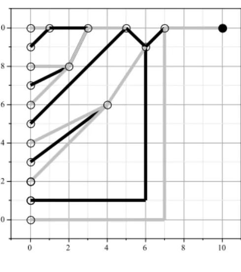
Fig. 1. A GB table of degree 6
Fig. 2. A GB of of degree 10 Moreover we say that a B table is a GB table if all the x-values of the end points of all the rectangles are pairwise distinct.
Theorem 13. Let f be a (P)-polynomial of degree n, and let m ≤ n be the number or real (simple) roots of f . Then m and n have the same parity, n = m + 2p and the Budan table of f is a GB table of degree n.
Example 1. Figures 1 and 2 show two GB tables: one of degree 6 with m = 0, p = 3 and the other of degree 10 with m = 4, p = 3. The first one corresponds to the polynomial f := int(F, x)+200, where ”int” denotes the integral and F := x5−12x4+42x3−53x2−28x−2.
Proposition 14. Let f be a (P)-polynomial of degree n. Consider a gray (resp. black) connected component bounded on the right of the Budan table of f . The x value of the rightmost (i.e top-right) corner of this component is a virtual root of f .
Let m ≤ n be the number or real (simple) roots of f , and let n − m = 2p.
There are p virtual non real roots of f , their virtual multiplicity is two; each of them is a root of some derivative of f of positive order.
We recover that f admits n virtual roots, counted with multiplicities.
Definition 15. We call augmented virtual root of f the pair (y, k) formed by a virtual root of f and n minus the order of the derivative of f which vanishes at y, i.e. f(n−k)(y) =
0. Notice that k is the degree of that derivative.
Remark 16. The augmented virtual roots of f depend only on the Budan table B of f . Virtual roots of a GB table are well defined.
Proposition 17. Let f be a (P)-polynomial of degree n.
By Rolle’s theorem between two successive roots a < b of some derivative f(m) with
0 ≤ m ≤ n − 2, (or in R if f(m) has no root), there is an odd number 2r + 1 of roots
(X2, ...X2r) are virtual non real roots of f .
Similarly if a is the smallest (resp. the largest) root of f(m), in the infinite interval
] − ∞, a[ (resp. ]a, ∞[) there is an even number 2r of roots (X1< ... < X2r) of the next
derivative f(m+1). Then the r roots with an odd index (X
1, ...X2r−1), (resp. the k roots
with an even index (X2, ...X2r)) are virtual non real roots of f .
For each augmented virtual non real root (y, k) of f , we have
f(k−1)(y)f(k+1)(y) > 0.
The following corollary explicits the relation between the virtual roots of f and f′
. Corollary 18. With the same hypothesis and notations.
The Budan table of the derivative f′
of f is obtained by deleting the first row of the Budan table of f .
Denote by (xi); 1 ≤ i ≤ u the ordered set of real roots of f and by (yj); 1 ≤ j ≤ v the
ordered set of virtual roots of f with order 1; call U the ordered union of these 2 sets. Then f′
has u + 2v − 1 real roots: the (yj); 1 ≤ j ≤ v and a set (zr); 1 ≤ r ≤ u + v − 1
of values in each of the u + v − 1 bounded intervals limited by the successive elements of U . The virtual roots of order k of f′
for k > 0 are the virtual roots of order k + 1 of f . Hence, the virtual roots of f and f′
satisfy the “classical” interlacing property. This was already noticed in (9).
3.3. Interpolation
Since it is monic, a (P)-polynomial f of degree n depends on n real coefficients, de-noted by a0, ..., an−1. However it has “only” m real roots and p virtual non real roots,
with n = m + 2p. In order to get the same number of parameters and constraints, we must attach to each of the p virtual non real roots another real value.
We choose to attach to each augmented virtual root (y, k) with k > 0 the value f(n−k−1)(y),
and so define a balanced system S of constraints.
Definition 19. We denote by S(f ) the system of n = m + 2p data formed by the m real roots (xi), 1 ≤ i ≤ m, of f ; the p augmented virtual root (yj, kj), 1 ≤ j ≤ p with kj> 0
and the p corresponding values wj := f(n−kj−1)(yj), 1 ≤ j ≤ p.
Notice that S(f ) defines a system of affine equations in the coefficients of f .
Two natural questions arise:
Is it true that two different (P)-polynomials f and g in Hn, define different systems
S(f ) 6= S(g) ?
Given a system S as above, does there always exists a (P)-polynomial f which satisfies these data ?
We will see that the answer to the first question is ”Yes” while the answer to the second one is in general ”No”.
The first question is a so-called homogeneous Hermite-Birkhoff interpolation problem, Hermite-Birkhoff interpolation, (HB) in short, is an old subject comprehensively reviewed till 1983 in the book (21). In contrast with Lagrange or Hermite interpolation, it does not always have a unique solution. In this theory, an important tool is the incidence matrix. 3.4. Incidence matrix
In HB theory, the list of constraints are written line by line, hence the rows of the incidence matrix correspond to real values where the functions are evaluated, and the columns correspond to degrees (or orders of differentiation). Since in our definition of Budan tables the roles of rows and columns are reversed, we will consider here the trans-posed of the usual HB incidence matrix. Yet the rows of the matrix are indexed (as usual) top-down.
Let h be the difference between two (P)-polynomials f and g having same augmented virtual roots and set of values wj : 1 ≤ j ≤ p, as above. Hence h has degree at most
n − 1, and its coefficients form n unknowns. It should satisfy n = m + 2p linear vanishing conditions: m corresponding to the m real roots of f and 2p corresponding to the p double virtual non real roots of f . We order the m + p distinct virtual roots y1< ... < ym+p of
f .
Definition 20. The incidence matrix E of a (P)-polynomial f only depends on the augmented virtual roots (yi, ki) of f . It is the (n, m + p)−matrix E = (ej,i) such that n
of its entries are 1, and the others are 0 according to the following rule: (1) If n − ki=0 then e1,i= 1.
(2) If n − ki> 0 then en−ki+1,i= 1 and en−ki,i= 1.
(3) Otherwise ej,i= 0.
Example 2. For a (P)-polynomial of degree 5, having one real root y2 and two
aug-mented virtual roots (y1, 2) and (y3, 4), with y1< y2< y3; the matrix E is:
0 1 1 0 0 1 1 0 0 1 0 0 0 0 0
In HB theory the following properties of the incidence matrix are extensively used. Definition 21. E satisfies Polya condition if and only if Mj> j for all j = 1...n; where
Mj denotes the sum of the entries in the first j + 1 rows of the incidence matrix E.
A maximal sequence of 1 in a column of E is called even (resp. odd) if the number of its elements is even (resp. odd).
E is said conservative, if and only if every odd sequence of E is non supported.
A maximal sequence of 1 in a column i of E starting at (j, i) is non supported if at least one of the two following sub-matrices of E (which can be void) does not contain any 1: - The upper left sub-matrix of E formed by the rows 1...j and the columns 1...i − 1 - The upper right sub-matrix of E formed by the rows 1...j and the columns i + 1...m + p.
In (3) it is proved that a homogeneous HB problem whose incidence matrix is both conservative and satisfies Polya condition, has only the trivial solution. See also (20) for simpler proofs.
Proposition 22. The previously defined matrix E (attached to m + p augmented virtual roots) is conservative and satisfies Polya condition.
The corresponding homogeneous HB problem has only the trivial solution. Hence the answer to the first previous question is “Yes”.
Proposition 23. Given a system S formed by pairs of real numbers and integers: (xi, 0)
with 1 ≤ i ≤ m, (yi, ki) with 1 ≤ i ≤ p, ki ≤ n, the set of values wi with 1 ≤ i ≤ p ,
n = m + p; there exist a unique monic polynomial F satisfying the conditions : F (xi) = 0, 1 ≤ j ≤ m+, F(n−ki)(yi) = 0, 1 ≤ j ≤ p , wl:= F(n−ki−1)(yi), 1 ≤ i ≤ p.
Remark 24. • The (yi, ki) with 1 ≤ i ≤ m + p, are not necessarily the augmented
virtual roots of F , as illustrated by the following Example 3.
• The invertible matrix of the linear transformation is a generalization of a Vandermonde matrix, see the following Example 4.
Example 3. Consider the general degree 3 monic polynomial F := x3+ a
2x2+ a1x + a0.
Require that y1 := 0 is a root of F , y2 := 1 is a root of F′, and the extra condition
F (1) = w.
The 3 constraints are: a0= 0, 3 + 2a2+ a1= 0, 1 + a2+ a1= w.
The solution is: a0= 0, a1= 2w + 1, a2= −w − 2.
Then y2 := 1 will be a virtual non real root of F , if and only if f (1)f′′(1) > 0. This
means w(w − 1) < 0, hence 0 < w < 1.
Notice that for w = 0, f admits a double real root at 1 and that for w = 1, f′ admits a
double real root at 1.
Hence the answer to the second question is “No”.
Example 4. The generalized Vandermonde matrix corresponding to Example 2 is a (5, 5)-matrix with entries monomials in (y1, y2, y3). Its determinant D(y1, y2, y3) is a
polynomial of degree 5 which does not vanish if the indeterminate are real and pairwise distinct.
D(y1, y2, y3) = 12(y1− y2)2((y1+ y2− 2y3)2+ 2(y1− y3)2).
Fix a GB table of degree n, through the set of its m + p augmented virtual roots, it defines an incidence matrix E. Hence with a set of values (wl) ∈ Rp, it defines a system
of constraints S.
Proposition 25. The set W of values (wi) ∈ Rp such that the system S represents a
(P)-polynomial, form a semi algebraic set (possibly empty) in Rp. More precisely, if we
fix the signs σ of the (wi) ∈ Rp such that the system S represents a (P)-polynomial, then
3.5. Realizable configurations
A question similar to interpolation is to ask if any GB table B of degree n is realizable, i.e. does there exists a (P)-polynomial f of degree n, which admits B as its Budan table?
The answer is ”No” because there are quantitative inequality between the roots of a polynomial and its derivative; see (23). So we need to weaken the requirements.
V. Kostov, in (18), proved that any sequence of numbers of roots of the derivatives, compatible with Rolle’s theorem, is realizable. Then he investigated in a series of articles, ((15), (16), (19)) arrangements of roots, compatible with Rolle’s theorem. He proved that if we fix an order of derivation k, then all arrangements of roots of f and fk, compatible
with Rolle’s theorem are realizable. But he showed that in degree 4 any arrangement of the roots of all the derivatives, compatible with Rolle’s theorem are not realizable; more precisely only 10 out of 12 are realized. There is also a related work by B. and M. Shapiro (25).
An arrangement of the roots of all the derivatives, compatible with Rolle’s theorem is equivalent to what we will call a qualitative B table.
Definition 26. Given a B table B of degree n as above, we call qualitative version of B the table obtained by ordering the roots of f and all its derivatives, say zi with
1 ≤ i ≤ N ; then replacing zi by i. There are a finite number of such qualitative B tables
with fixed degree.
Since in Figures 1 and 2, we did not mention the values zi, they are indeed examples
of qualitative GB tables.
Hence we need to extract from a qualitative GB table discrete invariants in order to expect, with this weaker requirement, that all configurations are realizable.
A candidate can be the previous incidence matrix but we prefer the B-tree, defined in the next subsection, which keeps some of the information on the same-color-connected components.
3.6. B-tree
in this subsection we define our new invariant the B-tree. With the previous notations it is obtained, from a qualitative Budan table, by contacting the m + p same-color-connected components to obtain a bi-color tree with m + p nodes and n + 1 leaves. Figures 3 and 4 illustrate our construction with the trees corresponding to example 1. Definition 27. The B-tree extracted from a qualitative B table B of degree n is a bi-color tree constructed on a grid [0..m + p + 3, 0..n] as follows.
We position the n + 1 leaves at the points (0, i), 0 ≤ i ≤ n and color them alternatively in gray and black; (0, 0) is gray. The root of the tree is positioned at (m + p + 3, 0). The root of the tree, the nodes and the leaves are connected by colored edges which are the contraction of the the same-color-connected components of B.
K1 0 1 2 3 4 5 6 0 1 2 3 4 5 6
Fig. 3. A B-tree of degree 6
0 2 4 6 8 10 0 2 4 6 8 10
Fig. 4. A B-tree of degree 10 We say that the B-tree is decorated if the coordinates (i, ki), 1 ≤ i ≤ m + p of its nodes
are given.
The obtained tree is rooted on the right of the picture and can be drawn (as usual) with short branches.
From a node (i, n) corresponding to a simple root of f start two branches of different colors. From a node (i, ki) with n − ki> 0 corresponding to a virtual non real root of f ,
start three branches of different colors: the two extremal ones have the same color as the one of its stem and the middle one is of opposite color.
All the degree n strict hyperbolic polynomials (i.e. having n distinct real roots) have the same decorated B-tree. Since they have several qualitative Budan table, we see that the decorated B-tree is a strictly weaker invariant.
So we may ask the two following questions about realizable configurations.
Question 1. Let B be a GB table of degree n, does there exist a (P)-polynomial f of degree n, which admits the same decorated B-tree than B ? respectively the same B-tree as B ?
We conjecture that they are both true. Notice that the first question is stronger than prescribing the numbers of real roots in each row.
Definition 28. Let T (f ) and T (f ) denote the B-tree and the decorated B-tree asso-ciated to a (P)-polynomial f . For a fixed decorated B-tree T , respectively B-tree T , corresponding to a GB table of degree n, we consider the strata ΣT, respectively ΘT, of
Hn formed by all the (P)-polynomials f such that T (f ) = T , T (f ) = T . We denote by
Σ and Θ these two stratification of Hn.
Proposition 29. Each stratum ΣT, respectively ΘT, of Hn is a semi-algebraic set of
Proposition 30. The virtual roots of a the polynomials f in a stratum ΣT of Hndepend
analytically on the coefficients of f .
Question 2. Are the strata ΣT connected in Hn?
4. Proofs
This section provides the proofs of the statements of the previous section. In the proofs of each statement we keep the notations of that statement.
4.0.1. Proposition 11
It is precisely Lemma 10.2.2 of (24), its proof relies on a continuous representation of f by conjugated complex roots and Ostrowski continuity theorem, plus the use of discriminants.
4.0.2. Theorem 13
We consider the different conditions of Definition 12. Items 1 and 2 and the last condition are obvious. Let’s prove item 3.
By Lemma 1, each (non first) rectangle of row Li is connected to a rectangle of the
same color on row Li−1 located on its left. So, by induction, any rectangle is
same-color-connected to one of the (n + 1) first infinite rectangles on the left side of the table. Each black connected component is bounded on its right; so it has a rightmost upper segment (call x its abscissa): if it is on Ln, then x is a real root of f , else if it is on Li,
i < n, it is surrounded below above and on the right by gray rectangles. In this last case, the black component stops at (x, i) and we also consider that the gray component above the segment coming from the left stops at (x, i − 1) since it is in an affluent of the gray component coming from the right which continues upward. Therefore two components (a black one and a gray one) stop at the abscissa x. The same reasoning works for the gray components bounded on the right, exchanging the roles of gray and black.
Let l denote the number of real roots of f and p denote the number of rightmost upper segment of a same-color-connected component bounded on the right. Since the gray component containing L0is unbounded, there are n other tails moving upward from the
left side. Hence n = l + 2p. 4.0.3. Proposition 14
When a same-color-connected component stops, the jump in the Budan-Fourier count is 2 if the component is surrounded below above and on the right by rectangles of opposite color, while it is 1 if it stops on the top row.
4.0.4. Proposition 17
Here is the proof of the first assertion, the second is very similar.
Assume without loss of generality that between a and b, f(m)is positive. Then by Lemma
1, on the left of x1, f(m+1) is also positive and changes sign at each of its successive root,
so f(m+1) is positive at the right of X
2. Between X1 and X2, there are an odd number
2u + 1 of roots of f(m+2), denoted by Y
1, ..., Y2u+1. Then f(m+2)is positive at the right of
Y2u+1. Hence the rectangle ]X1..X2[ on Ln−mis black and we deduce that it is surrounded
4.0.5. Corollary 18 Apply Rolle’s theorem.
4.0.6. Proposition 22
E is conservative because the only columns with one 1, have the 1 situated on the first row; the other columns have two 1.
Polya condition is clearly satisfied for the first two rows, because if a polynomial f has no real root, then its derivative has a at least one real root, hence f has at least a virtual root of order 1.
Let ρjdenote the number of real roots of f(j), j ≥ 0. Then by Proposition 17, the number
λj, j > 0 , of virtual roots of order j of f is: λj =12(ρj−ρj−1+1). Each of them gives rise
to two 1 in E. The count of 1 in the first j + 1 rows of E gives: Mj = j +12(ρj+ ρj−1+ 1).
Hence Mj> j.
4.0.7. Proposition 23
Indeed the corresponding generalized Vandermonde matrix is invertible, by Proposi-tion 22.
4.0.8. Proposition 25
Consider p other extra constraints f(ki+1)(y
i) = zi, at the augmented non real virtual
roots. The new system S′ is solvable if and only if the 2p parameters (z
i, wi) satisfy a
set of affine relations. And we also require for each i, 1 ≤ i ≤ p the non linear inequality zi.wi> 0. The solution is a union of convex polytopes whose vertices depend rationally
on the yi, then we consider its projection on the (wi) space Rp. If we fix the signs σ of the
(wi), hence those of (zi), the solutions correspond to the intersection of an affine space
with an hyper-octant in R2p, that we project on Rp to get an open polytope.
4.0.9. Proposition 29
The proof of Proposition 25 gives semi-algebraicity by elimination of the (wi). ΘT is
a finite union of strata ΣT.
4.0.10. Proposition 30
The complex roots of f as well as the virtual roots of f depend continuously on the coefficients of f . But this dependency is analytic as far as the roots do not collide and create multiple roots. But this event cannot occur when f moves in a stratum ΣT, since
it is formed by (P)-polynomials.
5. Without condition (P)
In this section we consider the case where the condition (P) is not necessarily satisfied. In order to generalize the concepts and results presented in Section 3, we need to slightly adapt the definition of a Budan table.
5.1. Multiplicities and simplified Budan table
Definition 31. We call simplified Budan table of f , the table obtained from the Budan table of f by skipping the segments between any two adjacent rectangles of the same color on a same row. In other words, for any integer k the roots of f(k) with even multiplicity
are no longer indicated.
Theorem 32. Let f be a monic polynomial of degree n, and let m ≤ n be the number or real roots of odd multiplicity of f . Then m and n have the same parity, n = m + 2p and the simplified Budan table of f is a B table of degree n with m + p same-color-connected components.
Proof. Lemma 1 also applies when f or one of its derivatives admits multiple roots, and since we suppressed the segments corresponding to roots with even multiplicity, the endpoints of the rectangles only correspond to roots of f(i), 0 ≤ i ≤ n − 1 with odd
multiplicities. So we can repeat the argument of the proof of Theorem 13 replacing the word ”root” by the expression ”root with odd multiplicity”. 2
Proposition 33. Let f be a monic real polynomial of degree n. The x value of the rightmost upper segment of a connected component (either gray or black) of the simplified Budan table of f is a virtual root of f . The virtual multiplicities are counted as follows: • the multiplicities of events appearing along a same x−value are added,
• the multiplicity of a simple root of f counts 1,
• the multiplicity of a simple virtual non real root (i.e. it is not a multiple root of a derivative of f ) counts 2,
• the multiplicity of a multiple root of f of order k counts k,
• the multiplicity of a multiple virtual non real root which is a multiple root of order k of a derivative of f counts k if k is even, and otherwise k + s1s2 with the notations of
the second table of Proposition 4.
Definition 34. We call augmented virtual root of f a pair (y, k) formed by a virtual root of f and an integer 0 ≤ k ≤ n − 1 which form the coordinates of the rightmost upper segment of a connected component (either gray or black) of the simplified Budan table of f . So there are m augmented virtual roots of type (y, n), and p augmented virtual roots of type (y, k), with k < n, such that n = m + 2p.
Different augmented virtual roots of f can correspond to the same virtual root of f . 5.2. Incidence matrix and B-tree
The definitions of B-tree, decorated B-tree, qualitative version of a Budan table, and of the stratifications given in Section 3, apply verbatim for the simplified Budan table of a monic polynomial f , even if it (or one of its derivatives) admits a multiple root. Similarly we have:
Definition 35. To a simplified Budan table B of degree n of a monic polynomial f corresponds an incidence matrix E = (ei,j). Let m be the number of real roots of odd
multiplicity of f and m + p be the number of augmented virtual roots, such that n = m + 2p. Then E is a (n, m + p) matrix with n entries equal to 1 and the others to 0,
Fig. 5. Budan table of example 5 according to the following rule.
Let (i, ki) be a node of the decorated B-tree then:
If n − ki = 0 then e1,i= 1. If n − ki > 0 then en−ki,i= 1 and en−ki+1,i= 1. Otherwise
ei,j= 0.
Again we have, with the same arguments:
Proposition 36. The matrix E is conservative and satisfies Polya condition. The corresponding homogeneous HB problem has only the trivial solution.
Example 5. We consider the monic polynomial f := (x − 1)4g/20 of degree 7 such that
g := 20x3+ 10x2+ 4x + 1 chosen such that we have at x = 0: f (0) > 0, f′(0) = 0,
f(2)(0) = 0, f(3)(0) = 0, f(4)(0) > 0. The polynomial f also has a real root of order 4 at
x = 1 and another simple real negative root.
The simplified Budan table of f is shown in Figures 5.
5.3. Deformations
Conjecture 1. Let f ∈ R[X] be monic of degree n and T be its decorated B-tree. Then, there exists a P-polynomial g of degree n with the same B-tree.
To prove that we need to control the deformations of f at the multiple roots of f and of its derivatives. The requirement is to deform f into F such that if x0is a root of f(k)
of multiplicity r it gives rise near-by x0 to no root of F(k) if r is even and to only one
root of F (k) if r is odd.
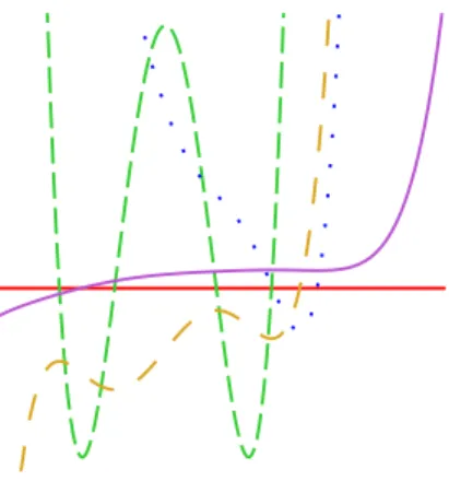
Example 6. For f as in example 5, the deformation F := x7+10.5x6+46.2x5+110.x4+
154.x3+126.x2+55.6x+10.4 of f gives the desired result. We constructed it by a sequence
of deformations and integrations starting from the third derivative of f . Figures 6 and 7 show the two families of graphs up to the third derivative.
Fig. 6. Graphs of the derivatives of example 5
Fig. 7. Graphs corresponding to the deformation
The stratifications Σ and Θ of Hn extends to En. The study of incidence relations
among the strata of Θ (or Σ) is an interesting question, but out of the scope of the present paper. A first task could be to answer the following question.
Question 3. Are the strata ΘT connected in En?
6. Conclusion 6.1. Extensions
In this paper, we have studied the same-sign-connected components of the Budan table of a univariate polynomial f , and extracted two types of information: the virtual roots which depend continuously on the coefficients of f and its Budan tree which is a finite discrete invariant attached to f . We related this construction to realizable configurations studied by V. Kostov and to Hermite-Birkhoff interpolation, which has received recently a renewed interest in Computer algebra, see (4). Then we defined a stratification of the space of polynomials and started its study. We left open several questions on the properties of the strata and their incidence relations. They provide directions for further investigations and experimentation.
There are other possibilities of extensions of the previous approach. 6.1.1. Algorithms for virtual roots isolation
In (14), we exploited the intersection of Budan tables with grids to develop algorithms for virtual roots isolation, and consequently a new method for real roots isolation of a univariate polynomial.
6.1.2. Fewnomials
In (9), the Budan-Fourier theorem and the continuity property of the virtual roots, were generalized to the case of Fewnomials, with a modified set of differentiations de-pending on a sequence of functions f .
More precisely, with our notations, our Lemma 2.1 and Proposition 2.4 are valid in that setting. Therefore our constructions can also be extended to that setting. In a joint paper
with Mariemi Alonso Garcia (2),for Issac 2012, we applied the method presented in this article to develop real roots isolation algorithms for sparse polynomials.
6.1.3. “Circular” differentiation
Another extension could be to replace the input polynomial f (x) of degree n by its homogenization F (X, Y ) in degree n, and then set X = cos(t), Y = sin(t) to get a trigonometric polynomial G(t) depending on n coefficients, hence G is periodic and takes bounded values in R. In that case, the derivative G′(t) of G(t) with respect to t can be
obtained similarly from another homogeneous polynomial.
Then we can define a periodic generalization of the Budan table, bounded on the columns and unbounded on the rows, but we can truncate it. There is again a generic case and one can study the corresponding “virtual roots” and B-trees.
6.2. Two more directions of research
• Study the relationship between virtual roots in an interval and pairs of conjugate complex roots, which lie in a sector close to this interval as initiated in Obreschkoff’s theorem, see (24), chapter 10.
• Investigate what happens if the coefficients of the input polynomials follow Gaussian random distributions. See (13).
References
[1] Akritas Alkiviadis G.: Reflections on an pair of theorems by Budan and Fourier, Mathematics Magazine, Vol. 55, No. 5, 292-298, (1982).
[2] Alonso-Garcia, M and Galligo, A : Real roots isolation for sparse polynomials. Proceedings ISSAC’2012, ACM; 35-42, (2012).
[3] Atkinson, K and Sharma, A: A partial characterization of poised Hermite-Birkhoff interpolation problems. SIAM J. Numer. Anal. vol 6 pp 230-236, (1969).
[4] Butcher, J.C and Corless, R.M and Gonzlez-Vega, L and Shakoori, A: Polynomial algebra for Birkhoff interpolants. Numerical Algorithms 56(3): 319-347 (2011). [5] Bemb´e, D: Algebraic certificates for Budan’s theorem. PhD thesis (2011).
[6] Bemb´e, D and Galligo, A: Virtual Roots of Real Polynomials and Fractional Deriva-tives. Proceedings of ISSAC’2011, ACM (2011).
[7] Bochnack, J. and Coste, M. and Roy, M-F.: Real Algebraic Geometry. Springer (1998).
[8] Budan de Boislaurent: Nouvelle m´ethode pour la r´esolution des ´equations num´eriques d’un degr´e quelconque. Paris (1822). Contains in the appendix a proof of Budan’s theorem presented at the Acad´emie des Sciences (1811).
[9] Coste, M and Lajous, T and Lombardi, H and Roy, M-F : Generalized Budan-Fourier theorem and virtual roots. Journal of Complexity, 21, 478-486 (2005).
[10] Dyn, N., Lorentz, G.G., Riemenschneider, S.D.: Continuity of the Birkhoff interpo-lation. SIAM J. Numer. Anal. 19(3), 507-509 (1982).
[11] Gonzalez-Vega, L and Lombardi, H and Mah´e, L : Virtual roots of real polynomials. J. Pure Appl. Algebra,124, pp 147-166, (1998).
[12] Galligo, A: Roots of the Derivatives of some Random Polynomials. Proceedings SNC’2011, ACM (2011).
[13] Galligo, A: Deformation of Roots of Polynomials via Fractional Derivatives. Ac-cepted for publication in JSC, 2012.
[14] Galligo, A: Improved Budan-Fourier Count for Root Finding. Preprint (2011). [15] Kostov, V.P.: Root arrangements of hyperbolic polynomial-like functions. Rev. Mat.
Complut. 19 (2006) no. 1, 197-225.
[16] Kostov, V.P.: On root arrangements of polynomial-like functions and their deriva-tives. Serdica Math. J. 31 (2005) no. 3, 201-216.
[17] Kostov, V.P.: On root arrangements for hyperbolic polynomial-like functions and their derivatives. Bull. Sci. Math. 131 (2007), no. 5, 477-492.
[18] Kostov, V.P.: A realization theorem about D-sequences. Comptes Rendus de l’Academie Bulgare Des Sciences, 60:12 (2007).
[19] Kostov, V.P.: On hyperbolic polynomial-like functions and their derivatives. proc. Roy. Soc. Edimburugh, Sect. A 137 819-8452 (2007).
[20] Lorentz, G.G., Zeller, K.: Birkhoff interpolation. SIAM J. Numer. Anal.vol8, 1, pp43-48, (1971).
[21] Lorentz, G.G., Jetter, K., Riemenschneider, S.D.: Birkhoff Interpolation, vol. 19. Addison-Wesley, Reading, MA; Don Mills, ON (1983).
[22] Muhlbach, G.: An algorithmic approach to Hermite-Birkhoff interpolation. Numer. Math. 37, 339-347 (1981).
[23] Peyser, G: On the Roots of the Derivative of a Polynomial with Real Roots. The American Mathematical Monthly , Vol. 74, No. 9 (Nov., 1967), pp. 1102-1104. [24] Rahman, Q.I and Schmeisser, G: Analytic theory of polynomials, Oxford Univ.
press (2002).
[25] Shapiro,B and Shapiro, M.: This strange and mysterious Rolle’s theorem. submitted to Amer. math. Monthly, arXiv: math CA/0302215.
[26] Vincent M,: Sur la r´esolution des ´equations num´eriques, Journal de math´ematiques pures et appliqu´ees 44 (1836) 235–372.