HAL Id: hal-00274017
https://hal.archives-ouvertes.fr/hal-00274017
Submitted on 17 Apr 2008HAL is a multi-disciplinary open access archive for the deposit and dissemination of sci-entific research documents, whether they are pub-lished or not. The documents may come from teaching and research institutions in France or abroad, or from public or private research centers.
L’archive ouverte pluridisciplinaire HAL, est destinée au dépôt et à la diffusion de documents scientifiques de niveau recherche, publiés ou non, émanant des établissements d’enseignement et de recherche français ou étrangers, des laboratoires publics ou privés.
Multigrid preconditioning of steam generator two-phase
mixture balance equations in the Genepi software
Michel Belliard
To cite this version:
Michel Belliard. Multigrid preconditioning of steam generator two-phase mixture balance equations in the Genepi software. Progress in Computational Fluid Dynamics, Inderscience, 2006, 6 (8), pp.459-474. �hal-00274017�
Copyright © 200x Inderscience Enterprises Ltd.
Multigrid preconditioning of Steam Generator
two-phase mixture balance equations in the
Genepi software
Michel Belliard
DEN/DTP/STH, CEA-Cadarache,
Bt 219, F-13108 ST Paul-lez-Durance, France E-mail: [email protected]
Abstract: Within the framework of averaged two-phase mixture flow simulations of PWR Steam Generators (SG), this paper provides a geometric version of a pseudo-FMG FAS preconditioning of the balance equations used in the CEA Genepi code. The 3D steady-state flow is reached by a transient computation using a fractional step algorithm and a projection method. Our application is based on the PVM package. The difficulties of applying geometric FAS multigrid methods to the balance equations solver are addressed. The effects on the convergence behaviour of the numerical parameters are investigated. An original parallel red-black pseudo-FMG FAS multigrid algorithm is also presented. The use of dynamic multigrid cycles leads to perceptible improvements in the computation convergences. Numerical tests (academic and industrial simulations) underline a noticeable computation speed-up, essentially for a large number of freedom degrees: the speed-up reached for 2 or 3 grids ranges between 2 and 3.
Keywords: two-phase flows; mixture; Steam Generator (SG); nuclear PWR; FAS; multigrid; finite element method.
Reference to this paper should be made as follows: Belliard, M. (xxxx) ‘Multigrid preconditioning of Steam Generator two-phase mixture balance equations in the Genepi software’, Progress in Computational Fluid Dynamics, Vol. x, No. x, pp.xxx–xxx.
Biographical notes: After obtaining his PhD in Theoretical Physics, M. Belliard joined the Genepi code team belonging to the Steam Generator (SG) Studies Department of the French Atomic Energy Commission (CEA). He is currently working on the multi scale/domain decomposition methods, such as multigrid algorithms, AMR methods, ADN methods and parallel solvers to achieve SG simulations equivalent to several million degrees of freedom.
1 Introduction
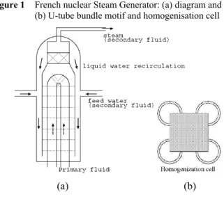
This paper provides an overview of a multigrid technique implemented in the CEA Genepi software (Grandotto and Obry, 1996; Obry et al., 1990). This software is dedicated to performing 3D simulations of steady two-phase flows in the riser of the PWR Steam Generator (SG), see Figure 1(a).
Figure 1 French nuclear Steam Generator: (a) diagram and (b) U-tube bundle motif and homogenisation cell
(a) (b)
Typically, a SG riser is a 10 m high and 3 m diameter cylinder, whereas the primary tube cell can be described as a 2 cm square, filled with 1 cm diameter primary tubes. Owing to this scale dispersion, a homogenisation technique is preferred to the complete fluid simulation between the obstacles, see Figure 1(b). Hence, the Genepi code solves the balance equations of an equivalent two-phase mixture in a porous-like media. A current challenge involves performing high space discretisation computations. Typically, we need several millions of elements to reach the primary tube cell dimension. An answer can be found in the Domain Decomposition Methods (DDM) (Belliard and Grandotto, 2002; Belliard, 2003). The implementation of DDM is built on the CEA coupling tool Isas (de Gramont and Toumi, 1996; Gulden et al., 1997) and the PVM library (kn:) with a master (Isas) – slave (Genepi) formalism. By implementing DDM, it is possible to carry out simulations involving a million cells with 20–30 processors, with each processor computing a 1,00,000 cells by sub-domain (about the maximum number of cells involved in a standard computation using one processor). In this context, new acceleration techniques are needed. Multigrid techniques can be a possible way to accelerate these computations
(Fedorenko, 1961; Bakhvalov, 1966; Brandt, 1977). For applications to the Navier-stokes equations, see for instance (Désidéri, 1998; Drikakis et al., 1998, 2000; Liu and Jameson, 1993). Roughly, a multigrid technique can be described as a solution method for (initially linear) systems, based on the restriction and interpolation of residuals, errors and approximations between a series of nested grids. As the equations to solve are strongly non-linear, the multigrid method specially dedicated to the non-linear equations is taken into account: the Full Approximation Storage (FAS) method (Brandt, 1977). This type of method has already obtained good results in the incompressible fluid dynamic framework (Désidéri, 1998).
This paper is organised into six sections. A two-phase flow model is detailed in Section 2. Section 3 reviews the multigrid architecture for the meshes and presents the FAS method. Section 4 is devoted to analysing some specific points of the FAS correction implementation for the mixture balance equations. Strictly speaking, the implementation of a geometric pseudo-Full Multigrid (FMG) version of the FAS method in Genepi is the object of Section 5. Finally, several numerical test cases are presented in Section 6, followed by some concluding remarks.
2 Two-phase flow modelling
The PDE set to be solved is the usual Navier-Stokes equation set for CFD with thermal exchanges and variable density (dilatable flow) (Obry et al., 1990; Grandotto and Obry, 1996; Aubry et al., 1989; Clerc, 2000): two-phase mixture mass, energy and momentum balance equations, see Equations (1)–(3). In our application, the stationary flow regime is reached by means of a pseudo-time marching (or similarly by the outer iterations of a relaxed Picard iterative method (Ferziger and Peric, 1996)). However, no time marching is applied to the mixture mass balance equation (the void waves are not taken into account). Hence, this approach leads to producing a solver that is very similar to those used in the incompressible fluid dynamic framework.
(βρv) 0
∇. = . (1)
In particular, at each pseudo-time step, a Chorin-like scheme (Gresho and Chan, 1990) (velocity prediction and projection steps) allows the simultaneous computation of the mixture mass flux and mixture pressure.
• Enthalpy balance equation
( . ) ( (1 ) ) ( ). t R T H v H div x x Lv Q div H βρ βρ β ρ β βχ ∂ + ∇ + − = + ∇ (2)
• Momentum balance equation
* ( * . ) * ( (1 ) ) * * ( ( * *)). t R R t T v v v div x x v v g v P div v v βρ βρ β ρ βρ β ρ β βµ ∂ + ∇ + − ⊗ = − Λ − ∇ + ∇ + ∇ (3) • Pressure equation 2 * P v t β δ ⎛δ βρ ⎞ ∇. ∇ = ∇.⎜⎝ ⎟⎠. (4)
The unknown are H, P and v v. * is the predicted velocity given the estimated pressure P* (Gresho and Chan, 1990). At each pseudo-time step δt, the balance equations are successively solved: energy (Eq. 2), predicted momentum (Eq. 3) and projection (Eq. 4) equations. The velocity and pressure are then updated:
2 * t v v δ δP ρ / = − , (5) * P=P +δP. (6)
Water thermodynamic tables are provided in order to compute ρ, x and L as a function of H and P. The µT, χT, Λ,
R
v terms are obtained using of a large set of semi-empirical closure relations (Obry et al., 1990). The most common relations are the Schlichting model for µT (µT = | |a G L where a is a
dimensionless constant, L is a typical vortex length, (Schlichting, 1968)) and the drift-flux Lellouche-Zolotar model (Lellouche and Zolotar, 1982) for vR, that is based
on the Zuber-Findlay approach (Zuber and Findlay, 1965). The heat source Q in the enthalpy equation is linked to the resolution of an energy balance equation for the primary flow (solved at the beginning of each pseudo-time step). To evaluate this term, other correlations on the heat exchange coefficient and the wall temperature are included.
Space discretisation is done by means of a Galerkine FEM (tri-linear Q1: H, v , β, G ; constant Q0: P) leading to a weighted integral version of the above-mentioned equations (weak formulation) in which the mechanical stress term and the energy diffusion term are integrated by part. Other physical quantities (i.e., ρ, x, µT, Λ …, ) are
included in Q0. The time discretisation is carried out using a Crank-Nicholson scheme. Diffusive terms are implicit, as is the frictional term (momentum). Generally speaking, the advective and drift terms are explicited. Like Gresho et al. we also included a Balancing Tensor Diffusivity (BTD) correction to increase the stability of the central difference advection scheme (Gresho et al., 1984). At each pseudo-time step, the arising linear systems are partially solved (5–20 iterations) by the preconditioned Conjugate Gradient method (CG, advective terms are explicit) or by the preconditioned Conjugate Gradient Square method (CGS, advective terms are implicit). However, the linear elliptic equation giving the mixture pressure is solved by LU decomposition.
According to the hyperbolic type of the flow equations, Dirichlet Boundary Conditions (BC) are used at the inlets of the domain (mass flux and enthalpy) and Neumann BC at the outlets (pressure). It is to be pointed out that the mass
flux (ρ is fixed because the user specifies the total mass v)
flow rate that has meaning from an engineering viewpoint. The other boundaries of the domain are impermeable walls. These boundaries are generally considered adiabatic with no shear stress (the strong pressure drop induced by the tube bundle leads us to disregard the wall shear stress).
This parabolic two-phase flow solver will be the smoother of our FAS algorithm. Hence, during a multigrid cycle m, a given number of pseudo-time steps n was performed.
The mixture qualifier for the flow will be omitted in the rest of the paper.
3 The FAS method
Within the framework of the weighted residual method, a typical problem is finding s (s ∈ V, V is a Hilbert space) which is the solution of:
( ) ( ) ( ) d 0
i i i
r s :=
∫
T sφ x v= ∀ ∈φ V (7)where {φi} is a basis of V, T(s) represents a non-linear
residual function of the solution s and ri(s) is the weighted
integral of the residual. If u is an approximation of the solution s, error is defined by e := s – u. Roughly speaking, a multigrid technique is an iterative method designed to solve this equation for a given grid Ω0 (here, called the finest grid; { }φ nodal base of Ω0), based on a series of 0i
successive estimations of the error on a hierarchy of nested coarser grids Ωl, 0 < l ≤ lmax where lmax represents the index
of the coarsest grid. In this section, the meaning of embedded meshes in a multigrid architecture will be recalled and the FAS method will be explained. Details will also be given on the restriction and prolongation operators used to transfer FE fields between the meshes.
3.1 The FE multigrid architecture
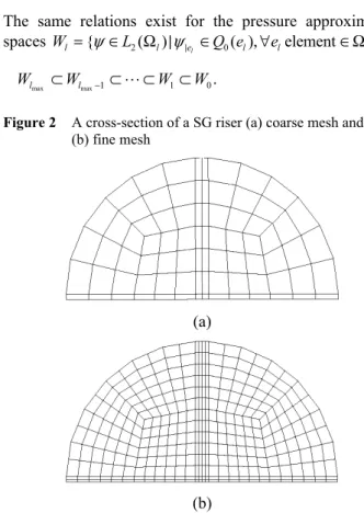
The embedded FE meshes are built as follows. Let there be a coarse Q1 FE mesh of a given computational domain, ΩH = {EH}, see Figure 2(a). Let it be that each coarse mesh
element is divided by r (e.g., 2) in each direction. Therefore, each hexahedral element is divided into r3 (e.g., 8) smaller ones and a finer FE mesh of the computational domain, Ωh = {Eh} is obtained, see Figure 2(b), with
H = 2h.
Using this process, all the coarse mesh nodes belong to the node set of the finest mesh and all the coarse mesh nodal functions i , H φ 1 1 { ( ) H ( ) } i H VH H H E Q EH EH H φ ∈ = φ∈ Ω |φ| ∈ ,∀ ∈Ω (8)
can be described by the nodal functions of the finest mesh , i h φ 1 1 { ( ) h ( ) } i h Vh H h E Q Eh Eh h φ ∈ = φ∈ Ω |φ| ∈ ,∀ ∈Ω . (9)
In other words, the FE function sets were embedded:
VH ⊂ Vh. Performing this refinement process recursively
drives to a embedded mesh set:
max max 1 1 0
l l
V ⊂V − ⊂ ⊂ ⊂ . (10) V V
The same relations exist for the pressure approximation spaces Wl ={ψ∈L2(Ω |l)ψ|el ∈Q e0( )l ,∀elelement∈Ω : l}
max max 1 1 0
l l
W ⊂W − ⊂ ⊂W ⊂W. (11)
Figure 2 A cross-section of a SG riser (a) coarse mesh and (b) fine mesh
(a)
(b) 3.2 The FAS method
A multigrid method (Brandt, 1977; Désidéri, 1998) – a Correction Scheme (CS) method for linear systems or a FAS method for non-linear systems – is based on a nested sequence of two-grid methods. In a two-grid method, discretised equations are smoothed on the fine grid Ω0 using a linear or non-linear iterative method. Fine-grid residual
r0(s) (and approximation u0 for FAS) are restricted 0 1
(R ) on the coarse grid Ω1 in order to compute error. This error is then prolongated 1
0
( )P on the fine grid to correct the fine-grid approximation. The two-grid algorithm stands as follows: we focus on our non-linear steady state equations to be solved, similar to Equation (7), the time terms are not taken into account. On the fine mesh Ω0, the discretised equation is: 0 0 0 0 0 0 ( ) ( ) di 0 i T s φ x x= ∀ ∈ +φ V BC
∫
(12)where V0 is defined by Equation (9), T0 is a non-linear discretised operator and s0 represents the sought solution on Ω0. We start the two-grid cycle with an approximation on Ω0: (u0)m, with m representing the cycle counter,
1 Only perform some passes of a smoother (cp0 iterations) for the fine mesh equation. We obtain the approximation 0
0
cp
u and the (non-linear, stationary)
residual 0 0 0 0 0 0 (rcp )T = −( ,…
∫
T u( cp ) ( ) d , ).φi x x… 2 Restrict 0 0 cp r and 0 0 cpu (FAS only) on the coarse mesh Ω1: 0 0 1 ˆ10 cp r r =R (13) 0 0 1 R u1 0cp u = . (14)
The two restriction operators are not the same (see below).
3 Solve (ideal method, black boxes in Figure 3 or smooth (non-ideal method, black circles) a corrected balance equation on the coarse mesh Ω1. The corrected equation is –V1 defined by Equation (8): 1( ) ( )1 1 1 1 1 I I I T u φ x dx S= ∀ ∈φ V
∫
(15) 1 1 1I 1( ) ( )1I I S =∫
T u φ x dx+r (16)Hence, a coarse mesh correction e1 is obtained and defined using the coarse mesh solution u e1: 1= −u1 u1
in the FAS case.
4 Prolong (interpolate) the coarse mesh correction on the fine mesh and correct the fine mesh approximation (α is a relaxation coefficient): 1 0 0 1 e =P e (17) 0 1 0 0 0 ( )u m+ =ucp +αe. (18)
5 Test the convergence. If this is not satisfactory, then a new multigrid cycle is to be used.
Figure 3 Multigrid cycles
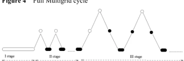
The multigrid algorithm consists in replacing the coarse-grid solver (Step 3) of the two-grid algorithm by calling a nested sequence of two-grid methods involving coarser grids. Several multigrid cycles can be defined (e.g., see Figure 3). In the FMG cycle version, instead of starting the multigrid cycle from the finest grid Ω0, the process begins with the coarsest grid (see Figure 4). Several coarsest
grid Ωlmax iterations are performed to reach a prescribed
error level. The prolonged approximation is then used as initial data to begin a two-grid algorithm on the finer grid
max 1
l −
Ω . After reaching a prescribed error level on this grid, the prolonged approximation is used once again as initial data to start a three-grid algorithm on the grid Ωlmax−2 and so
forth. This method provides a very good approximation on the finest grid in order to start the multigrid cycle. During a multigrid cycle, on each level, the error value to be reached by the smoother is not necessary a fixed constant and may depend of the current grid level (Désidéri, 1998; Drikakis et al., 2000; Saulnier, 1997).
Figure 4 Full Multigrid cycle
There are two ways to construct coarse-grid operators T1(). The first way is to build a coarse-grid operator from the discretisations of the balance equations on the coarse grid Ω1 itself (geometric multigrid version). Thus, the coarse grid geometry is involved in the computation of the T1() operator. Discrepancies between the grids can arise in the case of space-length-dependant terms (i.e., geometric modelisation of obstacles). The second way is based on the fine-grid (Ω0) equation discretisation only, according to the definition (arithmetic multigrid version):
0 1
1( ) ( ) d :1 1i 1 0( 0 1) ( ) d .1i
T u φ x x = R T P u φ x x
∫
∫
(19)Only the geometric multigrid version is taken into consideration in this paper. The arithmetic version leads to a high coherence between the coarse-grid and fine-grid discretisations, but is more costly to implement it with a code-coupling tool involving many communications between the tasks (for each computation of T1u1).
The FAS method is essentially a sequential one. Parallel versions can be found in the BPX preconditioning method of Bramble et al. (1990). In the BPX method, restrictions of the finest grid approximation are first transferred to allthe grids. All the corrections are computed on the grids in a parallel manner. In other words, each length scale is corrected separately from the others. All the corrections then are prolonged on the finest grid to correct the finest approximation.
4 A pseudo-FMG FAS algorithm
Here, analysis concerning the specific aspects of the geometric FAS preconditioning of the balance equations (Eqns. 2–4) is carried out for our numerical scheme. Here, the u1 term of Equation (14) represents the enthalpy, the primary fluid temperature, the mass flux and the pressure.
Similarly, the r1 term represents the energy balance residual
and the momentum balance residual. It is to be pointed out that it was chosen to restrict the mass flux instead of the velocity in order to be compatible with the free divergence mass flux constraint. Similarly, the errors concerning the specific enthalpy, the primary fluid temperature, the mass flux and the pressure must be computed and prolonged on the fine grid.
After having provided the expressions of the correcting terms, restrictions and prolongation operators, it was decided to focus on the strong variations of the forcing terms following the space discretisation scale and the use of the FEM and the Chorin’s projection algorithm. Moreover, the specific treatment of the BC and the primary flow energy balance equation was also emphasised.
Except for the mass flux, the locations and values of the BC are the same for all grids. Concerning the mass flux at inflow (Dirichlet BC), it is important to maintain the fine-grid nodal mass flux values G across the embedded coarse grids. Because the inlet porosities may be different from these coarse grids, similar user-specified mass flow rates
inlet
( in )
S
Q =
∫
βGdS for all the grids lead to different inlet mass flux values. To avoid BC discrepancies between the grids, the fine-grid inlet mass fluxes and enthalpy values are restricted on the coarse-grid inlet nodes. By doing this, priority is given to obtaining identical inlet mass fluxes for nodes shared by different grids.The FAS method is not implemented for the primary fluid energy balance equation. This equation is very easily and quickly solved on the primary curvilinear grid. However, as it is implied in the RHS source term of the mixture energy balance equation, the fine-grid correction of the primary fluid temperature is useful to enhance the specific enthalpy convergence. Hence, a coarse-grid restriction and a coarse-grid error of the primary fluid temperature are computed. The curvilinear fine-grid temperatures are transferred on the fine grid-elements and sent to the coarse-grid task. The coarse-grid temperature errors are computed as element fields and sent to the fine-grid task. A fine-grid correction is then performed. However, as no FAS correction is used for the coarse-grid primary fluid energy balance equation, the fine-grid temperature convergence cannot be expected. Therefore, if this temperature correction is not stopped, the enhanced convergence benefit will be lost in terms of the enthalpy. The stoppingtime is chosen to be equivalent to twice the time need to flow along the primary tubes.
4.1 Coarse-grid correction terms We have to compute the i
l
S term of Equation (16) for the energy, momentum and mass balance equations. These terms are formed by two parts. The first term
( ) ( ) di l l l
T u φ x v
∫
is built using the restricted variables u . The second term is the restricted nodal residual and is completely defined by the chosen restriction, in this case,the nodal weighted average restriction. It is important to remember that the mass balance equation restricted residual is equal to zero because this equation is solved up to the computer precision on the finer grid. The fine-grid mass flow βl−1Gl−1 is always divergence-free, but generally this
is not true for the coarse-grid restricted flow.
The first parts of the correction terms are the coarse-grid residuals of the fully non-linear steady-state flow balance equations, built with the restrictions of the specific enthalpy Hl, the primary temperature Tpl, the mass flux
øverrightarrow Gl and the pressure Pl . The values of the
coefficients implied in these coarse-grid correction terms (denoted restricted coefficients) are evaluated using these restricted variables. For instance, the restricted density is defined by ρl( H P )l, l .
• Energy balance equation
( ) ( ) d d ( )[ ( ) div( (1 ) )] d ( ) ( )( ) i i l l l l l l l l l l R l l l i i l l l l l l T T u x v v x G H x x L v v x Q dv x H φ φ β β ρ φ β φ β χ ≡ .∇ + − − + ∇ ∇
∫
∫
∫
∫
(20) • Momentum balance equation( ) ( ) d d ( )[ ( ) ] d ( )[ ( (1 ) )] d ( )[ ( )] d ( ) ( ) . i i l l l l l l l l i l l l l l l l Rl Rl i t l l l l l T l i l l l l l T u x v v x v v v x div x x v v v v x P v v v x g BC φ φ β ρ φ β ρ β ρ φ β β µ φ β ρ ≡ .∇ + − ⊗ − ∇ − ∇ + ∇ Λ − − +
∫
∫
∫
∫
∫
(21) • Pressure equation ( ) E( ) d d E( ) ( ). l l l l l lG T u ψ x v≡ vψ x∇.β∫
∫
(22)Equation (22) is not solved directly, but the free-divergence projection of the gap mass flux is reinforced: (Gl−Gl).
Concerning the non-linear features, the weakness lies in the use of the coarse-grid pseudo-time step value in the computation of the BTD correction.
4.2 The restriction and prolongation operators Specific restriction operators l 1
l
R− are defined following the restricted quantities. The nodal variables (e.g., 1 1
i i l l
u− ≡G− )
are transferred by canonical restrictions:
1
i I l ul
u = −. (23)
Here, the fine-grid node i and coarse-grid node I are the same nodes. The nodal-function weighted integrals (e.g., weighted residuals rli−1) are restricted by weighted
1 ( ) 1 I i I l i l i x r r =
∑
φ −. (24)The variables by element e (e.g., pressure ulE−1≡Ple−1) are
transferred by means of volume weighted restrictions (here,
1
e l
V− are fine element volumes):
1 1 E E e e l l l l e E V u u V− − ∈ =
∑
. (25)The prolongation operator Pll−1 used is the tri-linear
interpolation. It is to be pointed out that the weighted mean restriction is the transposed operator of the prolongation operator. This operator couple verifies the rule to obtain a mesh-size independent rate of convergence, see Albers (2000) and references within:
2
P R
m +m > m (26)
where mP and mR are defined as the orders of the
interpolation plus one order used for prolongation and restriction (here, 2 + 1) and 2m is the order of the partial differential equation to be solved (here, 2).
4.3 Pressure computation
The pressure evolution in the Chorin-Gresho algorithm (Gresho and Chan, 1990) is based on successive updates of an initial coherent pressure distribution. This initial pressure
P0 is obtained by a Consistent Pressure Poison Equation (CPPE) solver (Gresho, 1991) using an initial mass flux G0.
The latter is built from a user guess mass flux (see below). Next, a pressure update is performed at each free divergence space projection. The mass flux based on the solution v* of
the discrete version of the linearised predicted momentum balance equation (Eq. 3) can be expressed as
* ( n n) *.
G =ρ H P v, Solving the discrete version of the pressure equation (ref pressure equation), the pressure and mass flux updates read:
1 ,* ( ) d 2 d e i i n i e i P v G G t v δ βφ δ βφ , + ∇ = − /
∑ ∫
∫
(27) and , 1 , e n e n e P + =P −δP (28)with n representing the pseudo-time step counter. It is important to remark that there is a minus sign in Equation (28) owing to the integration by part of the stress term. Moreover, at the beginning of the computation, the free divergence constraint must be satisfied for the initial mass flux G0. Based on a given mass flux Guser and using a Lagrange multiplier technique (Gresho et al., 1984), a free divergence mass flux G0 can be found, as near as possible to Guser. In fact, the correction to be applied is similar to Equation (27) correction substituting Gn+1 (respect. G*) by
0
G (respect. Guser).
This initialisation procedure is used as a guideline to design a mass flux and pressure update step after the FAS correction steps on coarse and fine grids.
On the fine grid, two error terms can be potentially prolonged from the coarse grid: the mass flux error and/or the pressure error. Simultaneously applying these two error corrections breaks the coherence between the velocity and the pressure. The mass flux error correction is applied and then a new fine-grid pressure field solving the CPPE is computed, before running the Picard iterations.
On the coarse grid, after the fine-grid restriction at the beginning of the new multigrid cycle (m + 1), the
initial state of the fluid has to be defined seeing that
the reference divergence has changed: ∇.βGm+1, see Equation (22). A projection of the mass flux in the prescribed divergence space must be done in first, follow by a CPPE solve. More precisely, at the end of the previous multigrid cycle m (pseudo-time step n), we have (strong formulation): 1 m n n G G G β β − β ∇. = ∇. = ∇. , (29) 1 n n n n G G P O t β β δ − − = − ∇ + , (30)
where On stands for all the other momentum balance
equation terms not mentioned. Hence, the following is obtained: n n P O β ∇. ∇ = ∇ . (31)
( *, *)G P shall represent the mass flux/pressure couple after the change in the reference divergence (beginning of the multigrid cycle m + 1 and the pseudo-time step n + 1). Without changing the reference divergence, this initial couple would be equivalent to (G Pn, n). With change, this new couple should satisfy:
1 * m G G β β + ∇. = ∇. , (32) 1 * * * n G G P O t β β δ − − = − ∇ + (33)
with *O computed based on ( *, *).G P To enforce the new divergence constraint, the Lagrange multiplier technique (Gresho et al., 1984), produces:
1 m m G G β λ β β + ∇. ∇ = ∇. − ∇. , (34) * n . G =G − ∇ (35) λ
Let δP = P* – Pn. If we approximate *O by On (negligible
changes in viscous, convection and gravity terms), it can be deduced that:
1
( P t) Gm Gm
β δ δ β β +
It can be observed that Equation (36) is similar to Equation (34) with λ replaced by δPδt. Hence, the new pressure can be deduced directly from enforcing the new reference divergence field:
* n P P t λ δ = + . (37)
Remark: This algorithm can be understood as a standard
pseudo-time step computation to obtain the couple (G Pn, n) from the (Gn−1,Pn−1) couple, followed by a rapid start step
computation to obtain (G P*, *). The latter is described by
an acceleration arbitrary large for a very short time,
see (Gresho, 1991), using a similar hypothesis: viscous and
non-linear terms to be negligible:
* n G G P t β β δ δ − = − ∇ . (38)
Hence, Equation (33), may be written as follows (using the same δt for the two steps):
1 * n n n n n G G G G P P O t t β β β δ β δ δ − − + − ≈ − ∇ − ∇ + . (39)
4.4 Porosity and forcing terms
In our geometric version of the FAS multigrid method, the porosity and spread obstacles fields are independently computed on each grid. A unique inner technological device description is used (U-tube bundle, U-tube support plates, … described by a mesh) with several computation domain meshes: one by grid Ωl. On each grid, intersections
between the computation domain cells and the U-tube bundle/U-tube support plates are carried out, leading to the computation of the porosity and obstacle fields. Consequently, these fields are different in discontinuity regions (e.g., boundaries of the U-tube bundle) following the considered grid or equivalently the geometrical scale addressed. Hence, the forcing terms may differ strongly. For example, friction forces (induced by the U-tube bundle or the support plates included in the cell) may be applied to a
coarse-grid node, but not to the equivalent fine-grid node, see Figure 5.
Figure 5 Forcing terms
Moreover, the geometric approach to determine the coarse-grid forcing terms limits the total number of grids involved in the multigrid computation. For instance, three grids is the maximum for a 250,000-cell computation. As a matter of fact, with hexahedral elements in 3-D geometry, the coarsening ratio between two consecutive grids is 8 and, for a four level multigrid algorithm, the cell number ratio between the finest and the coarsest grid is 84 = 4096. Hence, the coarsest grid for this computation should only contain about 60 cells. The quality of the simulation would be very poor. In this case, it limits the multigrid algorithm to only three grids.
4.5 Dynamic multigrid cycle
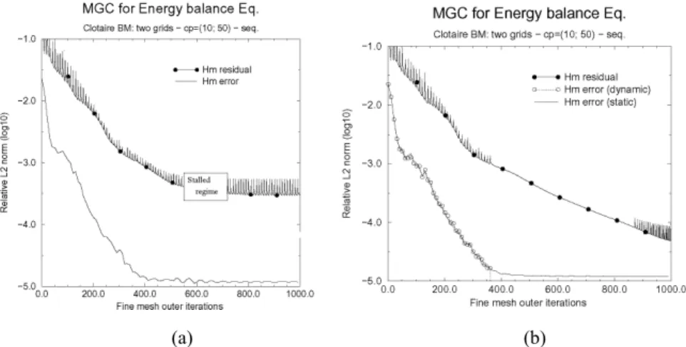
Because the coherence of the several formulations between the grids is not generally assumed, the error reduction associated with the high efficiency of the multigrid solver is drastically reduced after some cycles. It leads to the stalled regime illustrated in Figure 6(a). It shows the typical evolution of the relative error of the fine mesh enthalpy and of the energy balance equation residual during a static cycle FAS two-grid computation. After 400 pseudo-time step iterations (≡ 40 two-grid cycles),the magnitude of the error reaches 10–5 and no longer decreases. However, as mentioned in the numerical result section, about 60% pseudo-time steps of a Genepi standard computation were saved to reach this residual magnitude.
Figure 6 Pseudo-FMG FAS two-grid cycles: evolution of the energy residual and enthalpy error. Clotaire mock-up simulation; 22,400 cells (a) static cycle and (b) dynamic cycle
To overcome this drawback, the decrease in the error needed to be tested and the multigrid cycles required being dynamically managed. The goal is to go back to the standard Genepi algorithm, without FAS corrections of the fine-grid variables, as soon as the stalled regime is detected. The following coarse-grid indicator set indl (Ωl, l = 1, … lmax) is recommended: 1 2 2 2 (| | | | ) ( ) | | m m l l L L l l ref l L abs e e ind e e − − = (40)
where el represents the coarse-grid error (enthalpy or mass
flux), m is the multigrid cycle counter, ||L2 denotes the
discrete L2-norm, ref 2
l L
e
| | is a reference L2-norm (here,
1 2
l L
e
| | ) and abs(...) represents the absolute value function. The fine-grid Ωl–1 correction is monitored by the stalled
regime detection of the coarse-grid Ωl computed error. For
each coarse-grid task, dynamic multigrid cut-off criteria
MG l
ε can be set. The default value (user managed) for an industrial SG simulation is 5 × 10⁻³ for the specific enthalpy error criterion, whereas the mass flux criterion is based on the latter multiplied by a given factor (one by default). When a coarse-grid Ωl error verifies:
( ) MG l l l
ind e <ε , (41)
a FAS correction is no longer applied for the fine-grid Ωl–1
balance equation concerned by this variable. And when, this condition is reached both for the specific enthalpy and the mass flux, the coarse-grid Ωl task is halted. Figure 6(b)
shows the convergence of the fine mesh enthalpy error in the same test case as in Figure 6(a). After 37 two-grid cycles, the above criterion is satisfied for the enthalpy and a FAS correction is no longer applied to the fine-grid energy balance equation.
4.6 Computer implementation
The computer implementation of the pseudo-FMG FAS algorithm is based on a CEA code-linker tool denoted Isas (de Gramont and Toumi, 1996). In a master-slave context, the user defines several coupled boundaries for each Genepi slave (one task by grid). In the case of the FAS method, the
coupled boundaries involve all the nodes of the
computational domains, except the nodes associated with a Dirichlet BC. The master Isas collects such information and sends the corresponding external requests to the slaves. At each coupling iteration, the slaves simultaneously send the requested data, following the boundary condition nature of the external requests. These requests are balance equation corrections (coarse grid) or error corrections (fine grid). Next, each slave receives its own data to refresh the values of their coupled boundaries. After that, all the tasks perform some pseudo-time steps (not necessary the same amount cpl, l = 0, …, lmax) during the smoother step.
A sequential two-grid pseudo-FMG FAS computation begins by a coarse-grid solving without FAS correction during the first 0
1
cp pseudo-time steps (user managed).
If this number is big enough (of the same magnitude that the pseudo-time step number required to solve the coarse-grid problem alone), a true FMG method is obtained. If it is only equal to the current number of pseudo-time steps cp1, then a pseudo-FMG method is obtained. After that, the non-ideal FAS two-grid slash-cycles begin.
5 A parallel pseudo-FMG FAS algorithm
The two-grid pseudo-FMG FAS method presented above is essentially a sequential method. An easily implemented parallel version (in comparison of the BPX method) of our multigrid algorithm is found in a red-black colouring method. Several meshes named Ω0 (finest), …, Ω lmax (coarsest) were considered. Hereafter, the symbols ul,
l = 0, …, lmax, denote the variables (specific enthalpy and mass flux), wl the associated variables (primary fluid
temperature and pressure) and rl the steady-state non-linear
balance equation residual on the grids Ωl. Let us notice that
m multigrid cycles (denoted by (.)m+1) are equivalent to m
cpl pseudo-time steps (denoted by .(m+1)cpl).
A parallel algorithm – with simultaneous message exchanges between the tasks – is not compatible with an efficient multigrid correction. For instance, considering the previously described two-grid cycle (beginning with grid Ω1), the variable u0 at the end of the multigrid cycle m + 1 can be expressed as:
0 0 0 ( 1) 1 0 0 0 0 ( )m m cp ( m cp ) cp u + ≡u + ←It u +e (42) with * 1 ( * 1) 0 ( ) 1 0 0 0( 1 1 0 ) m cp m cp e =P u −R u − (43) * 1 * 1 1 ( ) ( 1) 1 ( 1 m cp m cp cp u =It u − ; * 0 * 0 * 0 ( 1) ( 1) ( 1) 0 1( 0m cp 0m cp 0m cp ) R u − ,w − ,r − (44)
where Itcp0( )... (resp. Itcp1(...,xxx)) denotes the action of
cp0 (resp. cp1) iterations of an iterative solver using the initial estimation ‘…’ (and involving a correction term build with ‘xxx’). We have m* = m + 1 for the sequential algorithm and m* = m for the parallel one. Essentially, replacing the index m* = m + 1 by m* = m in the error expression leads to an asynchronous corrections of the fine-grid approximation 0
0m cp
u at the beginning of multigrid cycle m + 1 (see Eq. 42):
0 1 0 ( 1) 0 1 1 0 0 1 0 0 1 (umcp −P R um− cp )+P umcp instead of 0 ( 1) 1 1 0 1 0 0 1 0 0 1 (I −P R u) mcp +P um+ cp
(sequential), with I0 representing the identity operator on the fine mesh vector space. In the latter expression, the fine-grid approximation low frequencies are corrected by the best available data. In the former expression, there is a multigrid
cycle shift between the fine-grid low frequencies and the coarse-grid correction.
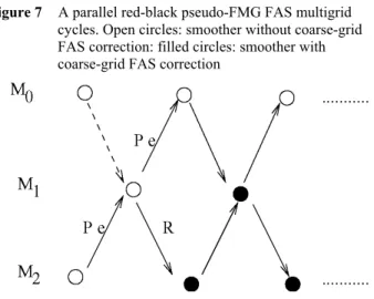
In order to retain the CPU time reduction benefit of a parallel coupling algorithm and the multigrid preconditioning acceleration, this naive new approach was developed, named the red-black pseudo-FMG FAS three-grid method, see Figure 7. As in a red-black Jacobi method, two groups of grids are set-up (e.g., {Ω0, Ω2} and {Ω1} with three grids). The two groups work sequentially and all the tasks of the same group work in parallel. The groups are set up in a way that two consecutive grids do not belong to the same group (odd and even numbers). Following this rule, a sequential non-ideal two-grid method is applied to each couple of consecutive grids.
Figure 7 A parallel red-black pseudo-FMG FAS multigrid cycles. Open circles: smoother without coarse-grid FAS correction: filled circles: smoother with coarse-grid FAS correction
A task related to an intermediate grid (e.g., Ω1) holds two
coupled boundaries associated with a coarse and a fine-grid
FAS boundary condition. The group holding the coarsest grid begins to work first. No coarse-grid correction is performed at the balance equations during the first multigrid cycle. At the end of the first cycle, the estimation of the approximation on the intermediate grid Ω1 results from a two-grid nested iteration computation. Similarly, with three grids, at the end of the second cycle, the estimation of the approximation on the finest grid Ω0 results from a three-grid nested iteration computation.
Hence, at the end of multigrid cycle m + 1, m > 0, the following can be expressed
0 0 1 0 0 ( 1) 1 1 0 0 0 0 0 1 1 0 ( )m m cp ( mcp ( mcp mcp )) cp u + =u + ←It u +P u −R u (45) with 1 1 2 1 1 0 0 0 ( 1) 2 1 ( 1) 1 1 1 2 2 1 0 1 0 0 0 ( ( ) ( )) mcp m cp mcp m cp cp mcp mcp mcp u It u P u R u R u w r − − = + − ; , , (46) and 2 2 1 1 1 2 ( 1) 1 ( 1) ( 1) ( 1) 2mcp cp ( 2m cp 2( 1m cp 1m cp 1m cp)) u =It u − ;R u − ,w − ,r − . (47)
The following remarks can be made: • The low frequency corrections of the
approximations are synchronised with the coarser grid values ( ) 1
1 l , 0 max 1: m cp l u ′ + l … l + = , , − 1 ( ) 1 1 1 1 ( l l ) mcpl l m cpl . l l l l l l I P R+ u P u+ ′ + + +
− + The index m′ is equals to m or m + 1 following the grid index l. Hence the fine-grid error correction spends between the sequential one (m′ = m + 1) and the parallel one (m′ = m).
• Concerning the intermediate grids, e.g., Ω1, the balance equation correction and the error correction terms are simultaneously applied. See Equation (46), leading to a loss of efficiency seeing that just after the correction of the Ω1 approximation, the RHS of the balance equation is modified.
As for the previously described pseudo-FMG FAS two-grid method, static or dynamic cycles can be addressed. In case of dynamic cycles, the relative variations of the errors defined on the coarse grids are monitored (Ωl with
max
1 l ).
l= , ,… Ω
6 Numerical tests
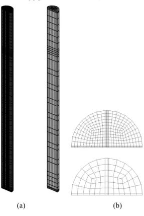
To test the implementation of the FAS method on SG two-phase fluid simulations, it was decided to present several sequential two-grid and parallel red-black three-grid computations belonging to the CEA Clotaire mock-up (Campan and Bouchter, 1988). Concerning this mock-up, the riser part forms a half cylinder of 0.62 m in diameter and 9.16 m in height. The inside is filled with a U-shaped tube bundle, 7.2 m in height, into which the hot primary flow enters. One flow distribution baffle, nine tube support plates and one anti-vibration bar are fixed respectively in the bottom, upright and curved part of the bundle. Figure 8 shows meshes of the inner technological devices used to compute the porosity filed: the plates and the U-tube bundle. The simulation fluid is Freon r114. The averaged mass flux is about 550 kg m–2 s–1 and the hydraulic diameter in the U-tube bundle is about 2 × 10⁻² m. Using this space step to mesh the riser leads to about 150,000 cells.
Except when specified, the BC and the physical and numerical parameters are identical for all computations (obtained from a Benchmark test case (Campan and Bouchter, 1988)). At the inlet the secondary total flow is split in cold leg and ıt hot leg parts with different specific enthalpies (resp. 1.185 × 10⁵ J kg–1 and 1.193 × 10⁵ J kg–1) and mass flow rates (resp. 28.3 kg s–1 and 37.55 kg s–1). These flows are mixed in the riser. The pressure is imposed at outflow (8.8 × 10⁵ Pa). The primary inlet mass flow rate is 60.05 kg s–1 at 361.8 K. The computation is stopped when each flow variable u (specific enthalpy, mass flux, pressure, primary fluid temperature) has verified the following steady-state flow criterion crit:
Figure 8 Clotaire inner technological devices (meshes) 1 2 2 | | | | n n L n L u u crit u δt + − ≤ (48)
with crit = 10–3 s–1 or 10–4 s–1. This latter ratio (multiplied by δt) is also used to describe the convergence of the flow variables in L2-norm. Standard numerical parameters for SG’s FAS computations are the following:
• cp0 = 15, cp1 = 60 and cp2 = 120 • pre conditioned Picard/CG smoother • α = 0.7, 3 1 10 MG ε = − and 3 2 10 . MG ε = −
Each fine grid is built by subdividing the coarser grid: each coarse-grid cell edge is cut into two parts, leading to eight times as many cells. Two fine grids are considered involving 22,400 cells and 88,704 cells. Numerical tests are performed on a heterogeneous PC cluster available in the laboratory and on the CEA supercomputer (Dec-Alpha ES40 stations with four EV68 processors). Typically, 20,000-cell computations are easily run on a PIV Intel processor (roughly one hour CPU time and 100 Mb) contrary to 100,000-cell computations roughly needing ten hours CPU time and 700 Mb on one EV68 processor.
Results are compared in terms of the total pseudo-time step number and total CPU and/or total elapsed time. The term
total refers to the sum of all tasks running in a sequential
manner. Both the CPU time overhead spent to initialise the coupling between tasks and the BC coupling phase (preparing data, sending, receiving and using new data) are also addressed.
6.1 A mixing pipe simulation
To begin with, our geometric version of the FAS multigrid scheme is tested in the best possible industrial configuration: i.e., without porosity and forcing terms discrepancies between the several grids. Hence, the simulation of a mixing flow in a pipe is addressed as a model problem. It is a simulation of a virtual ‘Clotaire’ mock-up, without any inner device, describing the mixing of
cold and hot flows in a vertical pipe of 9.16 m in height.
The set of balance equations is (1), (3) and (2) with β = 1, 0
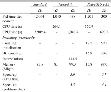
Λ = and Q = 0. Fine and coarse grids are shown in Figure 9(a) and (b) (real mock-up meshes). In Table 1, results from a standard computation (without FAS), a two-grid pseudo-FMG FAS computation and a two-grid nested iteration method one (coarse grid then fine grid computation, (Désidéri, 1998)) are compared.
Figure 9 Fine (22,400 cells) and coarse grids (2,800 cells) for the two-grid pseudo-FMG FAS computation of the mixing pipe: (a) 3D view and (b) cross-section view
Table 1 Mixing pipe simulations (steady-state: 10–3 s–1);
Pseudo-FMG FAS method: cp0 = 15, cp1 = 60,
α = 0.7, 4
1MG 10 ,
ε = − Picard/CG smoother;
crit = 10–3 s–1; 22,400 cells. One Ω
0 pseudo-time step
equals about 7.3 Ω1 pseudo-time steps
Standard Nested it. Psd-FMG FAS
Ω0 Ω1 Ω0 Ω1 Ω0 Psd-time step counter 2,064 1,040 488 1,201 300 CPU time (s) – 264.1 – 350.9 – CPU time (s) 3,909.4 – 1,046.6 – 693.2 Including (overhead): Coupling initialisation – – – 17.5 59.2 BC coupling – – – 16.9 30.6 Interpolations – – 114.5 – – Memory (Mbyte) 95.5 8.1 99.3 15.8 98.0 Speed-up (CPU time) – – 3.0 – 3.7 Speed-up (psd-time step) – – 3.3 – 4.4
Globally, as shown in Figure 10, the pseudo-FMG FAS method drastically reduces the amount of fine-grid pseudo-time steps needed to reach the steady-state. The speed-up value is equivalent to about 7. Of course, in terms of CPU time or total pseudo-time step number inferior, speed-up values are obtained (owing to the extra coarse-grid computation): 3.7 and 4.4 respectively. The CPU time overhead is about 10% of total CPU time owing to the data exchanges. The two-grid pseudo-FMG FAS method is clearly more efficient than the two-grid nested iteration method, even if coarse-grid computational work is slightly more demanding for the FAS method. For the two cases, obtaining the steady-state flow on the coarse grid requires about 1,000 pseudo-time steps (time for the physical propagation of the inlet information on the coarse grid).
Figure 10 Mixing pipe simulations: comparison of the
convergence histories of the fine-grid variables for the FAS method and the standard solver in L2 norm.
Pseudo-FMG FAS method: cp0 = 15, cp1 = 60,
4 1MG 10
ε = − , α = 0.7; Picard/CG smoother
The dynamic multigrid cycle cut-off criterion on the coarse grid is only reached at the end of the computation. Figure 11 shows the variations in the corrections of the fine-grid variables u, in the relative discrete L2 norm ((|unew – uold|
L2)/|uold|L2). This ratio can be as small as 10–4 or
10–6. Hence, it appears that no stalled regime is reached for the corrections of the variables. In the same figure, the discrete L2 norm of the fine-grid steady-state non-linearbalance equation residuals are shown. Several strong decreases in the energy balance equation residual can be observed each time the specific enthalpy correction is applied.
Figure 11 Mixing pipe simulations: convergence histories of the fine-grid variable corrections 1
0 1
(αP e) and non-linear residuals in L2 norm. Pseudo-FMG FAS method: cp0 = 15, cp1 = 60, ε1MG=10−4, α = 0.7; Picard/CG
smoother
Extra computations were carried out leading to the following remarks.
• In case of the Picard/CGS smoother (implicit convection term), the CPU time speed-up value is bigger due to the higher cost of the linear system solver: 4.1 instead of 3.7.
• The fine-grid error relaxation technique here is not a crucial point but slightly increases the method convergence: 3.7 instead of 3.5 (α = 1.0) for the CPU time speed-up.
• The FMG FAS method (defined by an initial run of 1,000 coarse-grid pseudo-time steps) is the best two-grid solver as expected and leads to the smallest number of fine-grid pseudo-time steps. Nevertheless, the work overhead on the coarse grid decreases the CPU time speed-up: 3.3 instead of 3.7 (pseudo-FMG). Hence, the pseudo-FMG approach is preferred. 6.2 A Clotaire mock-up simulation
Next, the simulation of the real Clotaire mock-up was examined. The porosity and the forcing terms present some discrepancies between the grids. Computations are performed with the sequential two-grid or parallel red-black
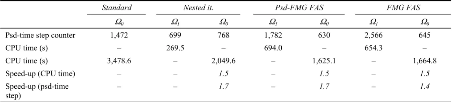
three-grid pseudo-FMG FAS methods. Table 2 displays results for the standard computation and two-grid methods: the nested iteration method, the pseudo-FMG FAS method
and the FMG FAS method. Figure 12 shows the convergence histories of the fine-grid flow variables with the pseudo-FMG FAS method.
Table 2 Clotaire mock-up simulations (steady-state: 10–3 s–1); sequential two-grid FAS method: 22,400 cells, cp
0 = 15, cp1 = 60
(first cp1 = 900; FMG FAS) α = 0.7, ε1MG=10 ,−3 Picard/CG smoother. One Ω0 pseudo-time step equals about 7.3 Ω1
pseudo-time steps
Standard Nested it. Psd-FMG FAS FMG FAS
Ω0 Ω1 Ω0 Ω1 Ω0 Ω1 Ω0
Psd-time step counter 1,472 699 768 1,782 630 2,566 645
CPU time (s) – 269.5 – 694.0 – 654.3 –
CPU time (s) 3,478.6 – 2,049.6 – 1,625.1 – 1,664.8
Speed-up (CPU time) – – 1.5 – 1.5 – 1.5
Speed-up (psd-time step)
– – 1.7 – 1.7 – 1.4
Figure 12 Clotaire mock-up simulations: comparison of the convergence histories of the fine-grid flow variables for the two-grid pseudo-FMG FAS method and the standard solver in L2 norm. Pseudo-FMG FAS method:
22,400 cells, cp0 = 15, cp1 = 60, 1 103 MG
ε = − , α = 0.7;
Picard/CG smoother
As shown in the table, the overall performances of the nested iteration method and the pseudo-FMG FAS method are similar for this test case. It is to be pointed out however that the number of fine-grid pseudo-time steps is smaller for the FAS method, which highlights better convergence properties. However, the pseudo-FMG FAS algorithm needs twice the coarse grid pseudo-time steps than the nested iteration method, leading to the same speed-up. The CPU time speed-up is lower than in the case of the mixing pipe simulation: 1.5 instead of 3.7. As a matter of fact, the dynamic multigrid cycles are stopped before obtaining the 10–3 s–1 steady-state criterion and after this point, the standard method is run. This can be seen in Figure 13. It shows the variations in the corrections of the fine-grid flow variable
Figure 13 Clotaire mock-up simulations: convergence histories of the fine-grid flow variable corrections 1
0 1
((αP e)) and non-linear residuals in L2 norm. Two-grid pseudo-FMG
FAS method: 22,400 cells, cp0 = 15, cp1 = 60,
3 1 10 , MG ε = − α = 0.7; Picard/CG smoother 2 new old old u u u L −
and of the non-linear balance equation residuals in the relative discrete L2 norm. Consequently, the choice of a lower value for the steady-state criterion leads to a decrease in the FAS acceleration performances considering that the method is run: the CPU speed-up is equivalent to about 1.4 for the value 10–4 s–1.
Again, the true application of the FMG algorithm does not increase the CPU time speed-up: the number of fine-grid pseudo-time steps is roughly the same as for the pseudo-FMG FAS computation, with the first 900 coarse-grid pseudo-time steps leading to a CPU time overhead without compensation.
An important feature is the fine-grid correction of the primary flow temperature. It provides a substantial increase in the enthalpy convergence. Without correction, the specific enthalpy convergence is not as fast, owing to the coupling of the energy balance equation with the primary fluid equation and the physical time needed to propagate the primary flow information.
As a whole, the coarse-grid solution does not greatly accelerate the fine-grid computation in comparison to the mixing pipe test case with the same mesh; about 57% instead of 85% of the standard computation fine-grid pseudo-time steps are saved. This can be explained by the discrepancies between the grids concerning the porosity, the friction and the thermal source terms. They limit the decrease in the coarse-grid error: 0
1 1 0.
u −R u The minimum value and, thus, the dynamic multigrid cycle cut-off criteria are reached more rapidly, leading to a greater fine-grid computational effort seeing that the balance equations are solved by the standard method. As shown in Table 1, as soon as the coarse-grid computation is converged, the fine-grid also converges. This is no longer the case for the Clotaire’s simulation, see Table 2.
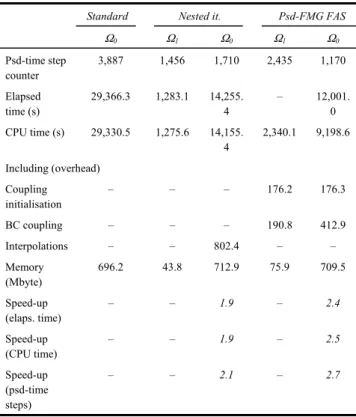
Tables 3 and 4 present the sequential two-grid and parallel red-black three-grid pseudo-FMG FAS results for the 88,704-cell test case. Computations are performed using the CEA supercomputer (one node by Genepi task). With the 88,704-cell mesh, the Ω0/Ω1 CPU time ratio is slightly larger than for the 22,400-cell mesh, which provides the MG methods with a greater advantage.
Table 3 Clotaire mock-up simulations (steady-state: 10–3 s–1);
sequential two-grid pseudo-FMG FAS method: 88,704 cells, cp0 = 15, cp1 = 60, α = 0.7, 1 10 ,3
MG
ε = −
Picard/CG smoother. One Ω0 pseudo-time step equals
about 8.4 Ω1 pseudo-time steps
Standard Nested it. Psd-FMG FAS
Ω0 Ω1 Ω0 Ω1 Ω0 Psd-time step counter 3,887 1,456 1,710 2,435 1,170 Elapsed time (s) 29,366.3 1,283.1 14,255. 4 – 12,001. 0 CPU time (s) 29,330.5 1,275.6 14,155. 4 2,340.1 9,198.6 Including (overhead) Coupling initialisation – – – 176.2 176.3 BC coupling – – – 190.8 412.9 Interpolations – – 802.4 – – Memory (Mbyte) 696.2 43.8 712.9 75.9 709.5 Speed-up (elaps. time) – – 1.9 – 2.4 Speed-up (CPU time) – – 1.9 – 2.5 Speed-up (psd-time steps) – – 2.1 – 2.7
Table 4 Clotaire mock-up simulation (steady-state: 10–3 s–1);
parallel red-black three-grid pseudo-FMG FAS method: 88,704 cells, cp0 = 15, cp1 = 60 cp2 = 120,
α = 0.7, 3 3
1MG 10 , 2MG 10 ,
ε = − ε = − Picard/CG
smoother. One Ω0 pseudo-time step equals about
8.4 Ω1 pseudo-time steps and 41.2 Ω2 pseudo-time
steps. Coarsest and finest grids run first
Standard Psd-FMG FAS
Ω0 Ω2 Ω1 Ω0
Psd-time step counter 3,887 2,202 1,773 1,005 Elapsed time (s) 29,366.3 – – 9,714.5 CPU time (s) 2,9330.5 510.3 1,752.0 7,800.3 Including Coupling initialisation – 3.6 179 175.8 BC coupling – 111.8 185.6 346.8 Memory (Mbyte) 696.2 10.1 76.2 709.5 Speed-up (Elaps. time) – – – 3.0
Speed-up (CPU time) – – – 3.1
Speed-up (psd-time steps)
– – – 3.1
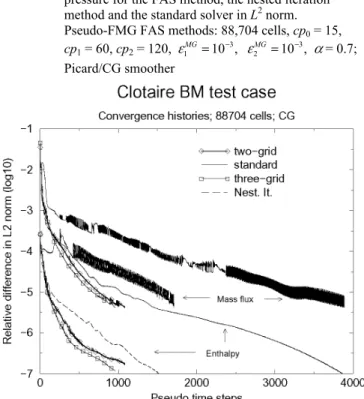
Figure 14 shows the convergences of the fine-grid flow variables. For this high space resolution computation, the performance of the pseudo-FAS method is higher than for the nested iteration method. More specifically, the saved fine-grid pseudo-time step number is noticeably higher, which counterbalances the bigger coarse-grid pseudo-time step number. The CPU speed-up is even greater than in the case of the 22,400-cell mesh: 2.5 (two grids) or 3.5 (three grids) instead of 1.5.
This can be explained by the already mentioned cheaper coarse-grid pseudo-time step cost and a lower efficiency of the standard method in terms of convergence (3,887 psd-time steps required to reach the steady-state criteria instead of 1,472). These points are related to the large number of degrees of freedom owing to the high space resolution. Using the parallel red-black three-grid pseudo-FMG FAS algorithm, the fine-grid (resp. intermediate-grid) pseudo-time step number is reduced once again in comparison with the sequential two-grid results: 1,005 instead of 1,170 (resp. 1,773 instead of 2,435). Moreover, taking advantage of a parallel run (Ω0 in parallel with Ω2), the three-grid computation elapsed time speed-up, the CPU speed-up and the pseudo-time step speed-up are all very similar. This supports the relevance of the parallel red-black pseudo-FMG FAS method for a large number of freedom degrees.
As with the 22,400-cell mesh, the dynamic multigrid cycle cut-off criterion is reached before the end of the fine-grid computation. The slope changes in the convergence curves, displayed in Figure 14, are related to the solver change (standard Genepi solver). Comparing three-grid and two-grid runs, the dynamic multigrid cycle cut-off criterion is verified about the same time for the mass flux: 25 multigrid cycles or 375 fine-grid pseudo-time steps.
However, the specific enthalpy criterion is verified at the same time for the three-grid run, instead of 35 multigrid cycles (525 fine-grid pseudo-time steps) for the two-grid run.
Figure 14 Clotaire mock-up simulations: comparison of the convergence histories of the fine-grid mass flux and pressure for the FAS method, the nested iteration method and the standard solver in L2 norm.
Pseudo-FMG FAS methods: 88,704 cells, cp0 = 15, cp1 = 60, cp2 = 120, ε1MG=10 ,−3 ε2MG=10 ,−3 α = 0.7;
Picard/CG smoother
Other computations using lower values of ε1MG lead to the
reduction in the fine-grid pseudo-time step number. However, this is counter-balanced by the increase in the intermediate grid pseudo-time steps …
6.3 Pseudo-FMG FAS method scalability
Scalability can be defined as follows. Let there be a problem involving nd degrees of freedom solved by a multigrid method using nt pseudo-time steps and a given number of 3D grids. If nd is multiplied by height and an additional grid is used, then the number of pseudo-time steps should be nt again.
Figure 15 shows the comparison of fine-grid mass flux convergences for the 88,704-cell three-grid, 22,400-cell two-grid and 2,800-cell one-grid computations. The figure also shows the convergences related to the 88,704-cell, 22,400-cell and 11,088-cell one-grid standard Genepi method computations. During the first 500 pseudo-time steps (active multigrid solver), it indicates a fairly good scalability of the pseudo-FMG FAS method. The following remarks can be made.
• Standard method computations show similar mass flux convergence behaviours for 22,400-cell and 11,088-cell test cases (about the same space discretisation
following the mean flow direction). This points to roughly similar convergences for the 11,088-cell and 22,400-cell two-grid pseudo-FMG FAS method.
• Subdividing a grid by two in each direction results in the doubling of the number of cells in the mean flow direction. As the CFL number is kept constant and the advection time needed to propagate information in the SG remains the same, convergence is two times slower for the standard solver when a grid is divided by 8.
• The 22,400-cell two-grid computation shows better convergence than the 2,800-cell one-grid standard solver computation. As the cp1/cp0 ratio is 4 and the pseudo-time step ratio is 2 (constant CFL number), 8 fine-grid pseudo-time steps onthe coarse grid are run for 1 on the fine grid, provoking an increase in the convergence. In fact, in the case of equal coupling periods (cpl = 20), the mass flux convergences are
closer, see Figure 17.
Figure 15 Clotaire mock-up simulations: comparison of the convergence histories of the fine-grid mass flux (L2 norm). Pseudo-FMG FAS method: cp
0 = 15, cp1 = 60, cp2 = 120, α = 0.7, 1 103 MG ε = − , 3 2 lonMG=10− ;
Picard/CG smoother. Scalability test
6.4 Relaxation of the FAS correction on the variables
Relaxation is a crucial point for the Clotaire mock-up simulation with the FAS method. Figure 16 shows the influence of choosing the relaxation parameter α for 22,400-cell two-grid computations. It is important to consider the mass flux convergence because it is generally the variable that demonstrates the slowest convergence. Clearly, choosing α in the range [0.4; 0.9] leads to similar mass flux convergence histories (even if [0.7; 0.9] seems the best interval). However, using a value of 0.95 deeply slows this convergence and a value of 1 (i.e., no relaxation) induces the divergence of the method. As the relaxation parameter value is not crucial for the mixing pipe test case, the grid discrepancies (porosity, …) may be pointed out.
Figure 16 Clotaire mock-up simulations: comparison of the convergence histories of the fine-grid mass flux (L2
norm) function of the relaxation parameter α. Pseudo-FMG FAS method: 22,400 cells, cp0 = 15, cp1 = 60, 1 10 ;3
MG
ε = − Picard/CG smoother
6.5 Choice of the coupling periods
An important question is choosing the coupling periods cpl.
Figure 17 illustrates this point for 22,400-cell two-grid computations. The dynamic multigrid cycle cut-off criterion is fixed at 10–5, allowing to catch all the convergence behaviours induced by the multigrid corrections. For the same reasons mentioned above, the scope is restricted to the mass flux convergence. It is to be remembered that the stalled regime is reached after about 1,000 fine-grid pseudo-time steps (except for the (cp0 = 15; cp1 = 60) computation) and, after this point, a standard method is run.
Figure 17 Clotaire mock-up simulations: comparison of the convergence histories of the fine-grid mass flux (L2 norm) function of the coupling periods cp
l.
Pseudo-FMG FAS method: 22,400 cells, 5
1 10 , MG
ε = −
α = 0.7; Picard/CG smoother
As a whole, all the convergence histories are spread near the coarse-grid standard solver convergence history and far away from that of the fine-grid. However, specific choices of the coupling periods can produce the best convergences. This is the case of the couple (15; 60). Moreover, some similarities in the convergence histories can be found. For instance, (15; 30) and (30; 60) lead to the same convergence. For these two couples, the coarse-grid/ fine-grid ratio is the same. Similar convergence properties can also be found for the couples (15; 60) and (15; 120). This last point underlines the fact that 60 coarse-grid pseudo-time steps are enough to solve the coarse-grid problem. In contrast, if the two coupling periods are too close each other, such as (20; 20) or (15; 30), the coarse-grid problem is not solved with enough accuracy, leading to a slower convergence on the fine grid.
Extra numerical tests have been performed on three-grid pseudo-FMG FAS computations. Results confirm the two-grid results and the 3-uplet (15; 60; 120) has been flagged as the best one.
6.6 Richardson as a smoother
A multigrid algorithm involves a smoother action on the fine meshes. It is necessary that this smoother both strongly dampen the high frequency component of the fine mesh approximations u0 and be economical. In the Genepi code, the smoother is provided by several relaxed Picard iterations (pseudo-time iterations) typically with 5 diagonal Preconditioned Conjugated Gradient (PCG) iterations. Richardson is a classical cheaper linear system smoother:
1
0 0 0( )0
j j j
u+ =u −αr u (49)
with r0(.) representing the fine-grid residual and j representing the Richardson iteration counter. However, the α parameter requires knowledge of the eigen values of the matrix. Because their estimations are not easily obtained and CPU time consuming, they are computed with the first CG step and kept constant during the Richardson sweep. Running a pseudo-FMG FAS two-grid computation using a relaxed Picard/diagonal preconditioned Richardson smoother (five Richardson iterations per fine-grid Picard iteration) produces similar results in comparison with the Picard/PCG results. Although an improvement of the smother action can be observed at the beginning of the pseudo-transien, no extra CPU time is really gained. Owing to the small contribution of the linear solver in a pseudo-time step, the mean-saved CPU time per fine-grid pseudo-time iteration is only equivalent to about 3%.
7 Concluding remarks
The FAS multigrid method has been successfully implemented and tested in the two-phase flow CFD Genepi code; showing better convergence than that obtained with a more intuitive method such as the nested method. Moreover, the greater the number of grid cells (here, one hundred