HAL Id: hal-01519969
https://hal.archives-ouvertes.fr/hal-01519969
Submitted on 9 May 2017HAL is a multi-disciplinary open access
archive for the deposit and dissemination of sci-entific research documents, whether they are pub-lished or not. The documents may come from teaching and research institutions in France or
L’archive ouverte pluridisciplinaire HAL, est destinée au dépôt et à la diffusion de documents scientifiques de niveau recherche, publiés ou non, émanant des établissements d’enseignement et de recherche français ou étrangers, des laboratoires
Void fraction in vertical gas-liquid slug flow: Influence of
liquid slug content
Sébastien Guet, Sandrine Decarre, Veronique Henriot, Alain Liné
To cite this version:
Sébastien Guet, Sandrine Decarre, Veronique Henriot, Alain Liné. Void fraction in vertical gas-liquid slug flow: Influence of liquid slug content. Chemical Engineering Science, Elsevier, 2006, 61 (22), pp.7336-7350. �10.1016/j.ces.2006.08.029�. �hal-01519969�
Void fraction in vertical gas-liquid slug flow:
influence of liquid slug content
S. Guet
1, S. Decarre
1,∗, V. Henriot
1and A. Lin´e
21 Institut Fran¸cais du P´etrole, D´epartement M´ecanique des Fluides,
1 et 4 avenue de Bois-Pr´eau, 92852 Rueil-Malmaison cedex, France.
2 Laboratoire d’Ing´enierie des Proc´ed´es de l’Environnement, D.G.P.E., I.N.S.A.,
135, Avenue de Rangueil, 31077 Toulouse cedex 04, France.
∗ Corresponding author. E-mail address: sandrine.decarre@ifp.fr
Abstract
In this study we develop a model for computing the mean void fraction and the liquid slug void fraction in vertical upward gas-liquid intermittent flow. A new model for the rate of gas entrained from the Taylor bubble to the liquid slug is formulated. It uses the work done by the pressure force at the rear of the Taylor bubble. Then an iterative approach is employed for equating the gas entrainment flux and the gas flux obtained via conservation equations. Model predictions are compared with experimental data. The developed iterative method is found to provide reasonable quantitative predictions of the entrainment flux and of the void fraction at low and moderate liquid slug void fraction conditions. With an increased liquid slug void fraction, experimental data indicate that the flow in the liquid slug transits to churn-heterogeneous bubbly flow thus gas entrainment flux tends to zero. Considering this effect in the iterative model significantly improved the predictions for large liquid slug void fraction conditions.
Key words: Gas-liquid, slug flow, slug aeration, gas entrainment, churn-bubbly, void fraction.
1 Introduction
In the oil industry, two-phase gas-liquid flow in pipes often leads to intermittent (or slug) flow, for which a large gas-pocket is, intermittently, followed by a liquid slug. Above critical values of the superficial gas and liquid velocities, the liquid slug contains dispersed gas bubbles. In vertical gas-liquid intermittent flow the pressure gradient can be expressed by: ∂P ∂z = β " ∂P ∂z # P + (1 − β) " ∂P ∂z # B , (1) in which β = LP
LP+LB is the Taylor bubble length fraction (LP is the length of the
Taylor bubble region and LB is the length of the bubbly liquid slug region). In the
Taylor bubble section the pressure is nearly constant thush∂P
∂z
i
P ≈ 0. In the liquid slug
section the pressure is essentially connected to the gravitational pressure (acceleration and friction contributions are small with respect to gravity). Provided the gas density is low with respect to the liquid density, the pressure gradient can be evaluated by
∂P
∂z ≈ (1 − β)²LBρLg, (2)
in which ²LB is the liquid fraction in the slug, ρL is the liquid density and g is the
acceleration of gravity.
Generally the liquid content in the Taylor bubble region is low in vertical gas-liquid
flows (the liquid film thickness is small), therefore ²LP
²LB << 1. Since the mean liquid
fraction is given by ²L = β²LP + (1 − β)²LB, (1 − β)²LB ≈ ²L and the (gravitational)
pressure gradient can be approximated by using the mean liquid fraction: ∂P
∂z ≈ ²LρLg. (3)
Therefore, using an empirical correlation for the mean void fraction in equation (3) can permit to successfully obtain a direct estimate of the pressure gradient in gas-liquid intermittent flow, without any required detailed parameter for the liquid slug. However equation (2) is in principle more accurate than (3) since no assumption on the liquid film thickness in the Taylor bubble region is needed. Furthermore in intermittent flow if the mean void fraction is to be modeled with a physically based approach, models for the flow in the Taylor bubble and in the liquid slug section should be used.
The aim of the present study is to develop a simplified physically based model for
predicting the mean void fraction in the liquid slug ²GB (= 1 − ²LB) and the mean void
fraction ²G (= 1 − ²L) in vertical co-current upward flow. Ultimately this model will
Slug aeration is essentially a function of the mixture velocity and of the tube diameter in horizontal flows and is correctly represented by the physically-based model of Andreussi and Bendiksen (1989) (Paglianti et al., 1991; Manolis et al., 1998; Orell, 2005). However inclination angle has a significant impact on slug aeration. For given flow conditions and fluid properties, liquid slug aeration increases significantly when increasing the inclination angle (Nydal, 1991; Nuland et al., 1997; Felizola and Shoham, 1995; Gomez et al., 2000; Zhang et al., 2003). As reported by Andreussi and Bendiksen (1989), their model for slug aeration is only valid for horizontal and slightly inclined flows, and does not take into account the significant increase of liquid slug void fraction with pipe inclination observed in the experiments.
To take into account the effect of pipe inclination on slug aeration, numerous semi-empirical models have been suggested in the literature. Felizola and Shoham (1995) suggested various coefficients in a set of fitting laws to take into account the inclination effects. Tengesdal et al. (1999) used a model fitting approach to obtain the slug aeration as a function of inclination angle and of the phases superficial velocities. Gomez et al. (2000) proposed an exponential power law to describe the effects of inclination. Zhang et al. (2003) proposed a model for slug aeration based on the hypothesis that the entrainment and break-up of bubbles at the rear of the Taylor bubble was due to the additional pressure gradient associated with momentum exchange between the slug body and the film zone. This model provided promising results, however the slug length fraction was used as an input parameter. In this perspective, it is of interest to develop a physically-based model for slug aeration which does not use the slug length as an entry parameter.
Also physically-based models using the conservation of gas and liquid fluxes have been developed (Fernandes et al., 1983; Lin´e, 1983; Nydal, 1991; Brauner and Ullmann, 2004). In these models the aeration of the liquid slug is obtained by modeling the en-trained gas flux at the rear of the Taylor bubble. A complete description of different regions of the flow and of the gas entrainment flux are needed in these models. The conservation of gas and liquid fluxes permits to close the model and to obtain pre-dictions for the mean void fraction. In this study we want to develop and test such a physically based model for the prediction of liquid slug aeration and mean void fraction in vertically oriented upward intermittent flow. Improved models will be developed for describing the flow in the liquid slug and for the entrained gas flux, and experimen-tal data will be used to check the validity of our models. The conceptual approach of Brauner and Ullmann (2004) based on an equilibrium of surface energy flux will be applied to model the gas entrainment flux at the rear of the Taylor bubble. Two mechanisms of gas entrainment will be considered: the turbulent ’jet’ present at the rear of the Taylor bubble (Brauner and Ullmann, 2004), and the work done by the pressure jump at the rear of the Taylor bubble.
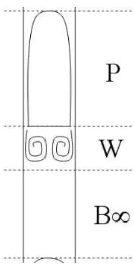
We consider that the flow can be separated in three parts (Brauner and Ullmann, 2004). These three parts are: the Taylor bubble region (P ), the Taylor bubble wake region (W ) and the developed liquid slug region B∞ (figure 1).
We assume that the flow is fully developed and at an equilibrium state, therefore the mean fluxes of gas and of liquid are equivalent at each boundaries:
ψG= ψGP = ψGW = ψGB∞, (4)
in which the gas fluxes are defined as:
ψG = ²G(VP − VG), ψGP = ²GP(VP − VGP), ψGW = ²GW(VP − VGW), ψGB∞ = ²GB∞(VP − VGB∞). (5)
These fluxes are given in a frame of reference moving at the Taylor bubble nose velocity
VP. ²G, ²GP, ²GW and ²GB∞are the mean void fraction in the whole section, in the Taylor
bubble region, in the wake region and in the developed liquid slug region. VG, VGP, VGW
and VGB∞ are the corresponding mean gas velocities.
In developed flow, also the liquid fluxes are equivalent, therefore
ψL= ψLP = ψLW = ψLB∞, (6) in which: ψL= ²L(VP − VL), ψLP = ²LP(VP − VLP), ψLW = ²LW(VP − VLW), ψLB∞ = ²LB∞(VP − VLB∞). (7)
²L, ²LP, ²LW and ²LB∞ are the mean liquid fraction in the whole section, in the Taylor
bubble region, in the wake region and in the developed liquid slug region. VL, VLP, VLW
and VLB∞ are the corresponding mean liquid velocities.
In the work of Brauner and Ullmann (2004), drift-flux relations with constant drift-flux parameters were used to model the gas and liquid velocity in the wake of the Taylor bubble and in the liquid slug. A model for the entrained gas flux at the rear of the Taylor bubble was suggested. The model of Brauner and Ullmann (2004) was shown to provide a reasonable description of slug aeration changes in inclined flows. Thus, such a model based on the conservation of gas and of liquid fluxes is expected to provide a robust approach for modeling the physics of slug flow hydrodynamics. However, as suggested by Brauner and Ullmann (2004), further research effort is required to establish the effect of the slug void fraction and tube inclination on appropriate values of the distribution parameter in aerated slug flow. The bubble entrainment phenomena at the rear of the Taylor bubble was attributed to the effects of the turbulent jet present at the rear of the Taylor bubble. Thus the turbulent kinetic energy of the jet present at the rear of
the Taylor bubble was used to express the gas entrainment-flux (Brauner and Ullmann, 2004). It might however be expected that gas entrainment can be described by another mechanism: the pressure jump present at the rear of the Taylor bubble (Nydal, 1991), necessary to accelerate the liquid from the film flow around the Taylor bubble to the developed liquid slug.
In the present study we will develop improved closure models for the flow in the liquid slug and these models will be included in an iterative approach based on the conser-vation of phase fluxes. Experimental data will be analysed to infer appropriate models for the mean velocities in the Taylor bubble wake and in the liquid slug for vertical upward flow conditions, and physical considerations will be developed to obtain upper and lower limit values for the mean void fraction and for the gas entrainment flux. An alternative physical mechanism for gas entrainment will also be studied: the work done by the pressure force present at the rear of the Taylor bubble (Nydal, 1991). As will be shown, an advantage of this gas entrainment model compared to the jet model, is that the liquid velocity in the wake is not needed. Our developments will be included in an iterative approach, and the predictions will be compared with experimental data from Nydal (1991), Koeck (1980), Ferschneider (1982) and Fr´echou (1986).
This manuscript is organised as follows: first, the experimental data used here will be presented. Upper and lower limit values for the void fraction and for the entrained gas flux will be derived and validated by experimental data. Also information about the mean gas velocity in the liquid slug and the entrained gas flux will be obtained from experimental data in section (2). This will enable us for conditioning our model and for developing appropriate gas velocity and flux models. In section (3) the basic principle of our model is described and the closure relations used in this study are explained. Possible gas entrainment mechanisms are discussed in section (4). Also criteria for the onset of gas entrainment will be discussed and formulated in this section. Then, we will make comparisons between experimental data and model predictions in section (5). Additional criteria for large void fraction conditions and large viscosity fluids will be suggested and compared with experiments in section (6).
2 Experimental data bank and simplistic modeling
2.1 Experimental data
The experimental data points used in the present study are the one of Nydal (1991), Koeck (1980), Ferschneider (1982) and Fr´echou (1986). The data of Nydal (1991) and Koeck (1980) are in particular interesting for studying the effect of liquid input, sur-face tension properties and pipe diameter on liquid slug aeration. Since these data are concerned with air-water experiments, additional data are needed to study the effect of viscosity. The data of Ferschneider (1982) are used for this purpose. Also the
ex-periments of Fr´echou (1986) are interesting for viscosity and surface tension effects: although most of the experiments of Fr´echou (1986) are conducted with a three phase flow of oil, water and gas, a few detailed experiments were reported for two phase flows of air and oil and of air and water. The same pipe was used in the two sets of experimental data.
Another interesting aspect of the data, is the way the experiments were achieved. In the experiments of Nydal (1991) and of Koeck (1980), the liquid input was kept constant and the gas input was increased progressively. Various liquid input conditions were studied using this approach (table 1). These particular conditions give us the opportunity of studying independently the effects of gas and liquid superficial velocities.
2.2 Simplistic modeling
2.2.1 Void fraction upper and lower limits
In vertical upward gas-liquid flows, the relative velocity between the gas and the liquid is positive (upward) in both the liquid slug part and in the gas-pocket, therefore the res-idence time of the gas-bubbles is smaller than the resres-idence time of the liquid. In these conditions, the mean void fraction associated with no slip homogeneous flow conditions (noted with the subscript nos) constitutes an upper limit for the void fraction:
²G,M ax = ²G,nos =
Usg
Um
. (8)
The gas flux in the frame of the moving Taylor bubble (at a velocity VP), is given by
ψG= ²G(VP− VG) = ²GVP− Usg. When there is no entrained bubble at the back of the
Taylor bubble, the gas flux is zero (these conditions are noted with the subscript nof ). At zero entrained gas-flux the mean void fraction reaches a minimum value, given by:
²G,min = ²G,nof =
Usg
VP
. (9)
It should however be noticed, that a zero gas entrainment rate does not neccesarly mean that the liquid slug is unaerated. Indeed, if the gas bubbles are convected at the
same velocity as the Taylor bubble, VP = VGB and ψGB = ²GB(VP − VGB) = 0 without
any required condition for ²GB.
In these relations, the Taylor bubble nose velocity is determined with the relation suggested by Nicklin et al. (1962):
VP = C0PUm+ 0.35 Ã (ρL− ρG)gD ρL !12 , (10)
in which C0P depends on the flow conditions (Fabre and Lin´e, 1992): C0P = 2.29 · 1 −Eo20(1 − e−0.0125Eo ) ¸ (11)
for laminar flow, and
C0P = logRem+ 0.309 logRem− 0.743 · 1 −Eo2 (3 − e−0.025Eo logRem) ¸ (12)
for turbulent flow. Here Rem = UνmLD and Eo = ρLgD
2
σ . Typicaly, in turbulent flow with
Rem > 8000 (ie. for air water flows at moderate and large mixture velocities), C0P
tends to 1.2.
2.2.2 Upper and lower limit estimates: validation
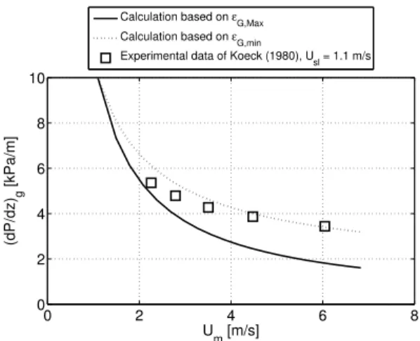
Following the formulation of the upper and lower limits for the mean void fraction, the upper and lower bounds are given by equations 8 and 9. As illustrated by figure 2 these expectations are validated by experimental data. In figure 3 the corresponding gravitational pressure gradient, calculated by using the lower and upper limits for the void fraction in equation 3, are presented. Although the pressure gradient can be approximated with this approach a more detailed model would be needed to gain accuracy in the pressure gradient estimates.
In figure 4 upper and lower limit estimates are compared with experimental data for the case of a viscous gasoil flowing through a pipe of diameter D = 7.37cm (Ferschneider, 1982). Also in this case the upper and lower limit estimates are in accordance with experimental data. In this case the data points are generally well described by the upper limit, which corresponds to the no gas entrainment flux assumption. This is actually in agreement with observations reported for such large viscosity fluids, for which generally no aeration of the liquid slug is reported (Fr´echou, 1986). In such case the liquid film flow in the Taylor bubble region is often laminar and the wake effects at the rear of the Taylor bubble are reduced (Campos et al., 1988; Pinheiro et al., 2000). These observations indicate that the gas entrainment flux tends to zero in such flow conditions.
2.3 Mean gas velocity in the liquid slug
In the liquid slug, the dispersed gas bubble velocity can be modeled by using the drift flux model (Zuber and Findlay, 1965):
In this relation the distribution parameter correctly describing the gas velocity is un-known for such conditions. Therefore, experimental data are used to infer appropriate drift-flux parameter models. Assuming no re-coalescence of bubbles, the gas-flux con-servation equation leads to:
²VP − Usg = ²GB(VP − VGB). (14)
We could not find any literature reporting direct measurements of the mean gas velocity in the liquid slug. However, using equation 14 the mean gas velocity in the liquid slug can be obtained :
VGB = VP −
²GVP − Usg
²GB
. (15)
This relation permits to study the best-descriptive law for the mean gas velocity in the liquid slug, by using experimental data reporting simultaneous measurements of the mean void fraction and of the liquid slug void fraction. The experimental data of Koeck (1980) are used for this purpose.
As noted initially by Zuber and Findlay (1965) in their conclusion, ”Plots in the velocity-flux plane which show abrupt change of slope and of intercept can be inter-preted as indicating a change of flow regime”. In heterogeneous bubbly flow conditions (or, similarly, in the ”churn bubbly” regime), Zuber and Findlay (1965) suggested the
use of the value C0B,Churn = 1.18. Hibiki and Ishii (2003) proposed a similar value for
the churn-bubbly flow, given by C0B,Churn = 1.2 −
qρ
G
ρL. This value is also comparable
to the value of C0P used in the Taylor bubble nose velocity (relation 10), therefore it
can be expected that when operating in the churn bubbly regime, the mean gas velocity in the liquid slug will be comparable to the Taylor bubble nose velocity. For homoge-neous bubbly flow, a value of order 1 was inferred by Zuber and Findlay (1965). For small bubbles and in the non-agitated bubbly flow, it was shown recently by Guet et al. (2003) and Guet and Ooms (2006) that at conditions where the radial distribution of void fraction is wall peaking the distribution parameter reaches a below unity value,
of typically C0B = 0.95.
In figure 5 the mean velocity in the slug bubble, calculated with equation 15, is shown
as a function of the mixture velocity for the experiments of Koeck (1980) at Usl =
0.7m.s−1
. Also predictions using C0B = 0.95 and C0B = 1.2 are shown. As can be seen
from figure 5 at increased mixture velocity the distribution parameter rises to a value of order 1.2. This result clearly indicates that the flow pattern in the liquid slug gradually evolves from a wall peaking, small bubble flow, to a core peaking churn-heterogeneous bubbly flow.
Another interesting aspect of this result, is that since the liquid slug gas velocity tends
to the gas-pocket nose velocity, the gas flux given by ψGB = ²GB(VP − VGB) tends to
void fraction (ψG = ²GVP − Usg) is plotted as a function of the mixture velocity. Also
the gas flux estimated by assuming an homogeneous wall peaking bubbly flow in the
liquid slug (C0B = 0.95) is represented. In the bubbly flow regime the entrained gas flux
increases with increased mixture velocity, and is well represented by using C0B ≈ 1.
However when the liquid slug is in the churn flow regime (ie. at Um > 2m.s−1 for the
experiments of figure 6), the gas flux is nearly constant and even gradually decreases with an increased mixture velocity. This observation on the maximum gas entrainment flux is also supported by the results for the mean liquid fraction (figure 2). At large mixture velocity the mean liquid fraction tends to the zero gas flux assumption result
(²L ≈ 1 − ²G,nof).
3 Model formulation: vertical intermittent flow
As explained in the introduction, an approach based on the conservation of phase fluxes is used. The approach suggested by Brauner and Ullmann (2004) is applied to separate the flow in three parts (figure 1): the Taylor bubble gas pocket (P ), the near wake zone in the liquid slug (W ), and the far wake zone (B∞). In this section we formulate models for the flow in these different regions.
3.1 Taylor bubble region (P )
We assume that the liquid film is free of gas and the liquid film flow is developed. The contribution of the nose region to the mean void fraction in the Taylor bubble section is neglected. The liquid film thickness is considered as small with respect to the pipe radius in vertical flow. Following these assumptions, the hydrodynamics of the liquid film can be described by a 2D falling film model. In addition the film flow is considered as fully developed and stationary. The force balance on a falling lump of fluid is then given by:
τw = ρLgδ, (16)
with δ the liquid film thickness and τw the shear stress at the wall. The wall shear
stress is given by τw = 12ρLflVLP2. For a laminar pipe flow fl = 16/Ref and for a
turbulent film flow we use Blasius relation, fl = 0.079Ref
−1
4. Here Ref = VLPDh
νl is the
film Reynolds number, based on the film hydraulic diameter (Dh = 4ASf
f = 4δ, with
Sf the wetted perimeter and Af the liquid cross sectional area). νl is the kinematic
Neglecting the contribution of the Taylor bubble nose the mean void fraction in the Taylor bubble section is given by:
²GP = Ã D − 2δ D !2 . (17)
Equation 16 and 17 are used to write a relation for the liquid film velocity VLP, valid
for a given liquid flux ψL. For a turbulent liquid film (Ref > 1000),
gD54 1 − s 1 −V ψL P − VLP 5 4 = Kturbνl 1 4VLP 7 4, (18)
with Kturb = 0.066. For a laminar liquid film (Ref < 1000),
gD2 1 − s 1 − ψL VP − VLP 2 = 8νlVLP. (19)
3.2 Developed liquid slug (B∞)
In the developed liquid slug, drift-flux relations are applied to compute the void fraction and phase velocities:
VGB∞= C0B∞Um+ U∞²LB∞
N. (20)
In the developed liquid slug (B∞), we assume the flow to be fully developed. It is first assumed that the liquid input conditions are such that turbulent break-up is determining the maximum bubble size in the developed liquid slug. Therefore, it might be assumed that at conditions where the liquid slug is aerated the corresponding bubble size is small and the radial distribution of void fraction in the liquid slug is wall peaking. As a result, we will first assume that the distribution parameter is constant and equal
to C0B∞ = 0.95.
The second term in the RHS of equation 20 is the weighted mean drift velocity and permits to take into account the effect of bubble drift velocity. In the present study
this term is taken as Vdrif t,B∞ = U∞²LB∞
N with N = 2.5 as suggested by Zuber and
Findlay (1965). The terminal velocity of a single bubble in an infinite medium, U∞, is
given by (Harmathy, 1960): U∞ = 1.53 ³σg(ρ L−ρG) ρL2 ´14 .
3.3 Wake region (W )
In the Taylor bubble wake region, the entering liquid jet leads to a negative liquid velocity in the near wall area. On the contrary, in the central zone of the liquid wake liquid recirculation due to the large vortex will result in an increased liquid velocity. This assumption is supported by experiments: in the central part of the near wake region, the liquid velocity is oriented upward, while in the near wall region the liquid velocity is negative (van Hout et al., 2002). The typical length of this wake region is one to five pipe diameters (Pinheiro et al., 2000; van Hout et al., 2002; Sotiriadis and Thorpe, 2005).
Following this observation, we assume that in the wake region and at the pipe centerline, the liquid velocity is equal to the gas-bubble rise velocity. At r = R−δ (δ is the thickness of the liquid film in the Taylor bubble region), it is assumed that the liquid velocity is zero. The minimum (negative) liquid velocity is taken as the (negative) liquid velocity of the liquid film. We also assume that the radial distribution of liquid velocity in the wake can be described by two parabolic functions. This assumption is consistent with available liquid velocity measurements in the wake of Taylor bubbles (van Hout et al., 1992, 2002; Nogueira, 2006), bubble column measurements (Mudde, 2005), as well as VOF-CFD calculations (Thorpe et al., 2001; Sotiriadis and Thorpe, 2005; Taha and Cui, 2006).
The radial distribution of liquid velocity is then given by:
vlw = vlw,1 = VP · 1 −³ r R−δ ´2¸ if r < R − δ; vlw,2 = VLP − 4VδLP2 h r −³R − δ 2 ´i2 if r > R − δ. (21)
Based on this formulation, the mean liquid velocity is obtained:
using VLW = A1 RAvlwdA, VLW = 1 2²GPVP + VLP²LP − 8VLP R2 δ2 · 1 4− 1 4²GP 2 − 2 3r˜min(1 − ²GP 3 2) + 1 2²LPr˜ 2 min ¸ ,(22)
in which ˜rmin = 1 − 2Rδ is the (dimensionless) radial position of the minimum liquid
velocity in the wake region.
This expression is found to provide reasonable estimates of the liquid velocity profile in the wake region. The shape of the functions (here parabolas) was not of primary importance for the mean liquid velocity determination: tests performed with flat profiles provided similar quantitative results for the mean liquid velocity in the wake. The most important aspect of this model is to consider the (negative) contribution of the liquid film velocity in the near wall region, on a layer of thickness δ. As will be illustrated in
section 5.1, this model is not equivalent to the use of a drift-flux model with a constant distribution parameter in the Taylor bubble wake zone.
3.4 Closure formulation
In the present approach, the model consists of 13 (independent) relations: • 1 relation for the Taylor bubble nose rise velocity (equation 10),
• 3 relations for the gas flux conservation (equation 4), • 3 relations for the liquid flux conservation (equation 6),
• for each of the 3 regions, hydrodynamics or drift flux models (equation 18 or 19, 20 and 22) (3 relations),
• 3 relations for linking the mean gas and the mean liquid fraction in each region
(²Gi+ ²Li = 1).
The unknowns of the system are: the Taylor bubble rise velocity, the mean void fraction in each of the three regions (3 unknowns), the mean liquid fractions (3 unknowns), the mean gas velocities (3 unknowns) and the mean liquid velocities (3 unknowns). Also the mean void fraction should be determined. Thus, there are 14 independent unknowns to determine and one additional relation is necessary for closing the model. This additional relation is introduced via a model for the rate of gas entrained at the rear of the Taylor bubble.
4 Gas entrainment flux modeling
4.1 Principle
In the present work it is assumed that the flux of surface energy is proportional to an energy supply, as suggested by Brauner and Ullmann (2004):
E = 6σ
d32
ψGe, (23)
in which ψGe is the volumetric flux of entrained gas. At equilibrium and assuming no
re-coalescence of bubbles into the Taylor bubble, the entrained gas flux ψGe is equal
to: ψGe = ψG.
We will further assume that the maximum stable bubble size dM ax, given by a critical
Bond number Boc = (ρL
−ρG)gd2
M ax
σ = 0.4 (Brauner, 2001), is equal to the Sauter bubble
diameter d32. Similar relations are applied in the gas entrainment model of Brauner
Various energy sources are possible. In particular, it is possible that this energy supply E is related to the turbulent ’jet’ present at the rear of the Taylor bubble (Brauner and Ullmann, 2004), or to the work done by the pressure forces. These two possibilities are studied here. The associated flux of energy supply is formulated and the model is used with these two approaches to inspect the validity of the associated entrainment mechanisms.
4.2 Entrainment flux due to turbulent jet (Brauner and Ullmann, 2004)
At the back of the Taylor bubble, the liquid flow forms a jet, which can be characterised by a net (relative) jet velocity. In the model of Brauner and Ullmann (2004) the energy source is attributed to the turbulent jet:
1 2ρL X ˙u2ψL = 6σ dM ax ψGe (24)
Here ˙u is the liquid velocity fluctuation, which is assumed to be related to the mean
jet velocity: P
˙u2 = 0.03(V
LW − VLP)2.
It is also expected that entrainment will only occur if the turbulent Weber number
W et =
ρLdM axP˙u2
3σ is above a critical value, taken as W ecrit =
2
3 by Brauner and
Ullmann (2004).
The model based on the turbulent jet assumption is then given by (Brauner and Ull-mann, 2004): ψGe= 1 400CJ dM ax D (W e − W ecrit)ψL, (25)
with a Weber number defined as W e = ρLD(VLW−VLP)2
σ . More details about the turbulent
jet entrainment model are given in the article of Brauner and Ullmann (2004).
4.3 Entrainment due to pressure jump at the rear of the Taylor bubble
We assume here that the pressure jump at the back of the Taylor bubble is responsible for gas entrainment. Thus, the gas entrainment flux results from a balance between the work done by pressure forces necessary to accelerate the liquid and the surface energy flux due to surface tension.
4.3.1 Pressure jump energy source
Only the acceleration pressure drop at the rear of the Taylor bubble is considered. The pressure drop necessary to accelerate the liquid from the gas-pocket section to the (developed) liquid slug is given by (Nydal, 1991):
∆P = ρL h ²LP(VLP − VP)2− ²LB∞(VLB∞ − VP)2 i , (26) which is re-written as ∆P = ρLψL(VLB∞− VLP). (27)
4.3.2 Critical conditions for entrainment
Since we consider in this section, that the pressure jump at the rear of the gas bubble is responsible for gas entrainment, liquid slug aeration is governed by a competition between pressure forces and surface tension forces. Therefore, the onset of entrainment should be described by a critical number:
·∆P τσ ¸ c = " ∆P dM ax σ # c = dM ax D [Eu.W e]c, (28)
in which the Euler number Eu is given by Eu = ρ ∆P
L(VLW−VLP)2.
We consider that only the excess of energy present above a certain limit, ie. Eu.W e >
[Eu.W e]c, results in gas entrainment. The critical value [Eu.W e]c should then verify the
following condition: if there is no gas, ie. Usg is zero, the liquid slug is not aerated thus
[Eu.W e] < [Eu.W e]c and ψGe = 0. For each experimental data point a corresponding
critical value [Eu.W e]cis found by first calculating Eu.W e for Usl= Um, ie. for Usg = 0.
4.3.3 Entrainment rate due to pressure jump
It is assumed that a proportion K∆P of the work done by the pressure force is used for
gas entrainment, and will then be available for surface energy transfer. Based on this assumption,
K∆PρL(VLB∞− VLP)ψL2 = CJ
6σ
dM ax
ψGe. (29)
The entrained gas flux is then given by:
ψGe= K∆PρL
dM ax
6σCJ
By including the critical conditions for entrainment (equation 28), the entrained gas flux is given by ψGe= K∆P 6CJ dM ax D (Eu.W e − [Eu.W e]c)ψL. (31)
4.4 comparison of the two gas entrainment approaches
Comparing the turbulent jet and the pressure jump assumptions, the two formulations can be related by:
ψGe,∆P = 67K∆PEuψGe,J et. (32)
Thus the Euler number gives a direct proportionality between ψGe,∆P and ψGe,J et. A
more detailed analysis of typical values taken by the Euler number showed that with our model and for the experiments considered in this study Eu ≈ 0.2, and Eu does not
significantly vary. Thus, it can be expected that provided K∆P and CJ are correctly
evaluated equation 25 and 31 will provide sensibly similar results. However, advantages of the method based on the pressure jump assumption are: the simplicity of the critical conditions for gas entrainment, and the use of the liquid velocity in the developed liquid slug. Indeed, the mean liquid velocity in the wake region is not necessary in the pressure jump model (equation 31).
4.5 Maximum gas entrainment
In vertical upward intermittent flow, the Taylor bubble is having a net positive upward rise velocity. Therefore, the mean void fraction is always less than the mean void
fraction given by an homogeneous no slip assumption: ² < ²nos =
Usg
Um. Since in the flow
conditions studied here VG and ² are by definition positive,
²G,nosVG> ²GVG= Usg > 0. (33)
Then the gas flux should verify
ψG= ²G(VP − VG) < ²G,nos(VP − VG) < ²G,nosVP − Usg. (34)
Therefore, the gas flux has a maximum value:
In our gas entrainment model, these additional criterion are applied by using:
ψG,entrainment= min(ψG,M ax1, ψGe). (36)
In section 6 we will also consider a maximum packing value for the void fraction in the
liquid slug, of ²GB,M ax = 0.55. This leads to a maximum value of the entrainment flux:
ψG,M ax2 = ²GB,M ax(VP − VGB). (37)
4.6 Model implementation
As listed in section 3.4, our approach consists in 14 unknown with 14 equations. It should be noticed, however, that when the pressure jump assumption is used to calcu-late the entrainment flux, the 4 flow properties of the wake region and its associated 4 equations are not necessary for computing the liquid slug void fraction and the mean void fraction. In this case the system of equation can therefore be reduced to 10 equa-tions with 10 unknowns, and the wake flow parameters are obtained once the system of equations is solved.
Our model is implemented in an iterative loop. The objective of this iterative model is to reach the equality:
ψG= ψG,entrainment, (38)
in which the entrained gas-flux is calculated with the models explained above.
First the starting gas flux values are calculated by using a starting guess for the mean
void fraction ²G = ²G,start. This starting value is taken as a mean value between the no
gas-flux assumption (²G,nof = UVsgP ), and the no-slip assumption (²G,nos = UUsgm):
²G,start = 1 2 µU sg VP + Usg Um ¶ . (39)
Then, iterations are carried out on the gas-flux by using the model consisting of the relations discussed in section 3.4 and of the gas entrainment model. At each iteration a new gas flux is calculated, which is a weighted average value of the previously calcu-lated value and of the entrained gas flux model result. Using this relaxation procedure permits to obtain a converged gas flux and prevents oscillations. Convergence criteria are applied to the model, based on a maximum relative deviation of the gas fluxes of
∆ψG
ψG and of the associated void fraction in the liquid slug
∆²GB
²GB of 0.001. With these
5 Results
In the present section we will discuss results obtained with the two gas entrainment models. The liquid slug content and mean liquid fraction are computed and compared with experimental data. The model used in this section is called the initial model.
5.1 Equivalent distribution parameter in the wake region
It is interesting to compare the results obtained with our model for the flow in the Taylor bubble wake with observations made in bubble column flows, where the liquid velocity is also reported to have negative values in the near-wall region. Hibiki and Ishii (2003) and Guet et al. (2004) report larger values of the distribution parameter in bubble column and low liquid input pipe flows compared to convected upward bubbly pipe flow. This is due to the presence of a returning flow in the near wall region. By using our method, we can calculate the equivalent distribution parameter in the wake by using the relation:
C0W =
VGW − U∞²LW
N
Um
. (40)
Such a result for the distribution parameter in the wake zone is presented in figure 7 for an air-water flow in a pipe of diameter D = 10cm. Indeed, with our profiles for the liquid velocity in the wake, the equivalent distribution parameter reaches large values
(C0W ≈ 1.4 at low input velocities). When the velocities are increased, the liquid down
flow is eventually suppressed, resulting in a decreased distribution parameter.
5.2 Void fraction
5.3 Void fraction in the liquid slug
In figure 8, predictions are compared with the experimental data of Koeck (1980) and in figure 9 similar comparisons are reported for the experimental data of Nydal (1991).
For the jet model equation 25 is applied with CJ = 1 (Brauner and Ullmann, 2004).
For the pressure jump model relation 31 is used and the coefficient K∆P was calibrated
to the experimental data. All the data points were used for this purpose. The value
K∆P = 10−2 was found to correctly describe the experiments and will be used in all
cases. As mentioned before the critical conditions for entrainment are computed by
As illustrated by figures 8 and 9, the comparisons between experimental data and itera-tive code predictions are reasonable. Generally the pressure jump hypothesis (equation 31) provides slightly better results than the jet model formulation (equation 25). These
slight differences are attributed to the use of a calibrated constant K∆P and an
im-proved model for the onset of entrainment. With adapted coefficients CJ and W ec and
improved models for the flow in the wake, it is expected that the two methods would provide more similar results, in view of equation 32.
5.4 Mean liquid fraction
Typical comparisons between developed liquid slug void fraction predictions and ex-periments were presented in figures 8 and 9. The comparisons were reasonable by using
K∆P = 10−2. However the results are not as satisfying with respect to the mean
liq-uid fraction. As illustrated by figure 10, at large mixture velocities the predictions are generally underestimating the mean liquid fraction by typically −50% when the void fraction in the liquid slug is correctly predicted (the measurements of Koeck (1980) at
Usl = 0.7m/s are also presented in figure 10, as in figure 8).
These simultaneous comparisons of mean void fraction and of liquid slug void fraction suggest additional effects to influence the void fraction at large mixture velocities. Pos-sible additional effects, which should be taken into account for proper comparisons with experimental data, are: the flow properties in the liquid slug, and the characteristics of the film flow. This will be the subject of the next section.
6 Additional considerations
In this section additional considerations are addressed. Essentially, these considerations concern the properties of the flow in the liquid slug and the character of the flow in the annular liquid film:
• the flow regime in the liquid slug seems to be best described by a ”churn agitated bubbly flow” model at large mixture velocity (section 2.3);
• with viscous liquids, the film flow properties might affect the gas entrainment value. This will be analysed with experimental data.
6.1 Homogeneous-bubbly to churn-bubbly flow transition
6.1.1 Experimental data information
As discussed previously in section 2.3, at some conditions the gas velocity in the liquid slug is best described by a ”churn-agitated” model (figure 5) and the entrainment flux decreases with an increased gas input (figure 6). A change from homogeneous to heterogeneous flow regime is observed at increased void fraction, similarly to bubble column flow conditions (L´eon-Becerril and Lin´e, 2001; Mudde, 2005). It is expected that the change from an homogeneous to an heterogeneous flow is, therefore, associated with an increased mean void fraction in the liquid slug. Since as discussed in section 2.3 these regimes are associated with different drift-flux parameter values, it is possible to detect this effect by estimating the equivalent distribution parameter for the flow in the liquid slug:
C0B =
VGB − Vdrif t
Um
, (41)
in which the mean velocity in the liquid slug is obtained from the experimental data,
using equation 15 with the measured values of ²GB and of ²G.
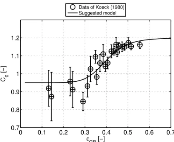
In figure 11 the results for the equivalent distribution parameter in the liquid slug are
presented. In this plot it was assumed that Vdrif t = 0.35√gD (Zuber and Findlay,
1965). The errorbars were calculated by assuming Vdrif t = 0. It is clear from this
picture, that the flow evolves from an homogeneous, wall peaking radial distribution of
void fraction with C0B ≈ 0.95, to an heterogeneous churn flow regime with C0B ≈ 1.15
at a typical critical value of the liquid slug void fraction of ²GB = 0.35. This result also
supports the consideration that the void fraction in the liquid slug is the most important parameter for determining the flow regime (experiments carried out at various liquid input conditions are reported on this plot).
6.1.2 Bubbly to churn-bubbly regime transition model
A model for the distribution parameter changes with liquid slug void fraction is sug-gested here. We consider that the transition takes place at a critical value of the liquid
slug void fraction given by ²GB,crit = 0.35. To take into account the gradual changes
from an homogeneous wall peaking bubbly flow to a churn agitated bubbly flow, we propose the use of the following relation:
C0B = C0B,wp 1 +³ ²GB ²GB,crit ´N + C0B,churn 1 +³²GB,crit ²GB ´N. (42)
In this relation, C0B,wp is the distribution parameter associated with wall peaking
homogeneous bubbly flow and C0B,churn is the distribution parameter associated with
churn-heterogeneous bubbly flow. As illustrated by figure 11, the changes of equivalent distribution parameter could be reasonably described by using this model. Here we used
N = 7, C0B,churn= 1.2 and C0B,wp= 0.95. Comparisons between associated predictions
for the mean gas velocity and experiments of Koeck (1980) at Usl = 0.7m.s
−1
are presented in figure 12. The model provides a reasonable description of the changes of mean gas velocity in the liquid slug.
In our iterative model, this bubbly to churn flow transition consideration is
imple-mented as follows: the drift-flux model value C0B = 0.95 used for describing an
homo-geneous model is replaced by equation 42. In this relation the value of the void fraction
in the liquid slug ²GB,churn is taken from the previous iteration. Then, relation 13 is
applied to compute the mean gas-velocity in the liquid slug. The associated gas-flux is calculated by using:
ψGB,churn= ²GB,churn(VP − VGB,churn). (43)
Using a larger value for C0B results in an increased gas velocity in the liquid slug.
With our model for the gas entrainment, this resulted in an increased void fraction in the liquid slug at large mixture velocity. The maximum packing condition (equation 37) was employed to limit the value of the liquid slug void fraction at large mixture velocity.
6.1.3 Results with the bubbly to churn-bubbly flow transition model
In figure 13 the gas entrainment calculated with and without this churn flow
consid-eration, is compared with the experimental data of Koeck (1980) at Usl = 0.7m.s
−1
. Taking into account this additional condition clearly improves the gas entrainment es-timates at large mixture velocity. It also permits to better predict the associated mean liquid fraction (figure 14).
In figure 15, we report comparisons of model predictions with all the measurements of the mean liquid fraction in air water systems (Fr´echou, 1986; Koeck, 1980). Both the initial model (without churn flow considerations) and the improved model predictions are displayed. It is clear from this result, that our model provides improved predictions of the mean liquid fraction, particularly at low liquid fraction conditions, where the void fraction in the liquid slug is large and the liquid slug operates in the churn-bubbly regime.
Only when the liquid viscosity was increased (eg. for the experiments of Ferschneider (1982) and of Fr´echou (1986) with oil), our model is found to underpredict the liquid fraction. Additional considerations on the properties of the flow in the falling liquid film and in the bulk liquid slug are addressed in the next section.
6.2 Influence of film flow properties: viscosity effects
Depending on the character of the liquid film flow, it can be expected that gas en-trainment will be observed or not. As was illustrated by figure 4, indeed for a number of experimental point the mean liquid fraction with the viscous fluid experiments of Ferschneider (1982) is well described by a no gas-flux assumption. To study this effect, experimental data associated with large viscosity liquids are analysed separately in this section. Model predictions with the initial model are compared with an improved model. In this improved model, we will assume that if either the liquid film or the bulk flow is laminar, gas entrainment is absent.
6.2.1 Viscous effects: model implementation
The conditions used for determining the laminar-turbulent transitions are the following:
• The film flow is turbulent for Ref > 1000 (Kockx, 2005).
• We consider that the bulk flow is turbulent provided Rem > 1200.
If the flow in the film or in the liquid slug bulk is laminar, we will consider that the entrained gas flux is zero.
6.2.2 Viscous effects: results
The experimental data of Fr´echou (1986) with viscous oil are used to study the effects of liquid viscosity. These data are interesting for this purpose, since typical values
associated with these experiments are Ref ilm = 250 − 500. Also, in these conditions
no churn flow in the liquid slug is expected since ²G< 0.4. It is thus possible to study
In figure 16 a comparison is made between the experimental data points and model predictions. The results obtained with the initial model are compared with results obtained by neglecting gas entrainment. Indeed, neglecting gas entrainment provides better predictions than the initial model. In this view, it is also interesting to notice that in numerous experiments with viscous fluids in moderate diameter pipes, the film
Reynolds number takes values in the range Ref = 200 to 1500, therefore the film flow is
in the transition region. Detailed measurements in these conditions would be of support to study the changes of gas entrainment rate during film flow transition.
7 Conclusions
A new physically based model was developed for predicting the hydrodynamics of gas-liquid cocurrent vertical upward intermittent flow. This new model employs the framework of the Taylor bubble wake model suggested by Brauner and Ullmann (2004). It includes an explicit formulation for the liquid velocity in the Taylor bubble wake region, a drift-flux formulation for the developed liquid slug part, and an hydrodynamic film model for the Taylor bubble region. Additional considerations are addressed with respect to lower and upper limits of the mean void fraction. Experimental data were used to study the existing flow regime in the liquid slug. It is found that the flow transits from wall peaking homogeneous flow to churn agitated bubbly flow when the gas fraction in the liquid slug is increased.
The existence of gas entrainment for laminar conditions in the film zone is also consid-ered, and our (iterative) model is used to test the validity of two assumptions for the mechanism of gas entrainment. These gas entrainment mechanism assumptions are: (1) gas entrainment is due to the inertial effects of the turbulent ’jet’ present at the rear of the Taylor bubble (Brauner and Ullmann, 2004), or (2) gas entrainment is to be associated with the work done by the pressure force necessary to accelerate the liquid from the Taylor bubble film region to the developed liquid slug. From the results, it is found that these two approaches provide similar results, since they are proportional
to similar quantities, ie. [VLW − VLP]2 and [VLB∞− VLP]2 . However the model based
on the pressure jump hypothesis provided sensibly better results. An advantage of this new gas entrainment formulation is that the wake region model is not needed to obtain mean void fraction information. The developed formulation for gas entrainment also included a model for the onset of gas entrainment. It is based on the simple considera-tion that gas entrainment can only exist when the gas input is different from zero, and provided a good description of the experiments.
At low and moderate values of the void fraction, as suggested by Brauner and Ullmann (2004) the mean void fraction in the liquid slug is essentially the result of a competition between the above mentioned gas-entrainment mechanism and surface tension. Indeed, in these conditions the liquid down flow in the film is large enough to guarantee small bubbles and the flow in the liquid slug is best described by an homogeneous model
based on the assumption of a wall peaking radial distribution of void fraction. When increasing the void fraction in the liquid slug, the bubble size increases and the flow is the liquid slug progressively transits to churn-agitated turbulent bubbly flow regime. The mean gas velocity is then best described by a churn flow model. At these large mixture velocity conditions, models for the mean gas velocity in churn flow are having a
formulation similar to the rise velocity of the Taylor bubble, therefore ψGB = ²GB(VP−
VGB) tends to zero. Also, in these conditions the void fraction in the liquid slug reaches
values of the order of the maximum packing value. Taking into account these effects is found to be crucial for proper mean void fraction predictions at large liquid slug aeration. A new model for the changes in the drift-flux distribution parameter in the liquid slug was suggested and tested on the experimental data. It clearly improved the accuracy of the predictions. Also the characteristics of the flow in the liquid film and in the bulk of the liquid slug are found to affect the aeration rate of the liquid slug. When the film flow or the bulk of the liquid slug is laminar, no liquid slug aeration is observed. This was taken into account in our model.
Finally, we should like to address an additional consideration concerning the length of the wake region. When operating at large mixture velocity the wake length might become, in some conditions, non negligible in comparison with the liquid slug length (Campos et al., 1988; Pinheiro et al., 2000). Thus the mean void fraction in the wake might contribute to the void fraction in the liquid slug. In experiments, it can be ex-pected that depending on the experimental techniques used, the wake contribution is included or not in the liquid slug content measurement results. More detailed measure-ments in the wake zone when operating in the churn agitated liquid slug regime would be of support to understand these effects.
Acknowledgments
S. Guet is grateful to F. Brucy, E. Heintz´e, E. Duret, M. Gainville and Y. Peysson for their interest and their support during this study.
References
Andreussi, P., Bendiksen, K. 1989. An investigation of void fraction in liquid slugs for horizontal and inclined gas-liquid pipe flows. International Journal of Multiphase Flow, 15, pp 937-946.
Brauner, N. 2001. The prediction of dispersed flows boundaries in liquid-liquid and gas-liquid systems. International Journal of Multiphase flow, 27, pp 885-910.
Brauner, N, Ullmann, A. 2004. Modelling of gas entrainment from Taylor bubbles. Part A: slug flow. International Journal of Multiphase flow, 30, pp 239-272.
Campos, J.B.L.M., Guedes de Carvalho, J.R.F. 1988. An experimental study of the wake of gas slugs rising in liquids. Journal of Fluid Mechanics, 196, pp 27-37. Fabre J, Lin´e, A. 1992. Modeling of two-phase slug flow. Annual Review of Fluid
Me-chanics, 24, pp 2146.
Felizola, H., Shoham, O. 1995. A unified model for slug flow in upward inclined pipes. Journal of energy resources and technology, 117, pp 7-12.
Fernandes, R.C., Semiat, R., Dukler, A.E. 1983. Hydrodynamic model for gas-liquid slug flow in vertical tubes. AIChE Journal, 29, pp 981-989.
Ferschneider, G. 1982. Ecoulement gaz-liquide `a poches et `a bouchons dans les con-duites de section circulaire. PhD thesis, Institut National Polytechnique de Toulouse, France.
Fr´echou, D. 1986. Ecoulement triphasique huile-eau air. PhD thesis, Institut National Polytechnique de Toulouse, France.
Guet, S., Ooms, G., Oliemans, R.V.A., Mudde, R.F. 2003. Bubble injector effect on the gas-lift efficiency. AIChE Journal, 49, pp 2242-2252.
Guet, S., Ooms, G., Oliemans, R.V.A., Mudde, R.F. 2004. Bubble size effect on low liquid input drift flux parameters. Chemical Engineering Science, 59, pp 3315-3329. Guet, S., Ooms, G. 2006. Fluid mechanical aspects of the gas-lift technique. Annual
Review of Fluid Mechanics, 38, pp 225-249.
Gomez, L.E., Shoham, O., Taitel, Y. 2000. Prediction of slug liquid holdup: horizontal to upward vertical flow. International Journal of Multiphase Flow, 26, pp 517-521. Harmathy, T.Z. 1960. Velocity of large drops and bubbles in media of infinite or
re-stricted extent. AIChE Journal, 6, pp 281-288.
Hibiki, T., Ishii, M. 2002. Distribution parameter and drift velocity of drift-flux model in bubbly flow. Int. Journal of Heat and Mass Transfer, 45, pp 707-721.
Hibiki, T., Ishii, M. 2003. One dimensional drift-flux model for two-phase flow in a large diameter pipe. Int. Journal of Heat and Mass Transfer, 46, pp 1773-1790. Hout, R. van, Shemer, L., Barnea, D. 1992. Spatial distribution of void fraction within
a liquid slug and some other related slug flow parameters. International Journal of Multiphase Flow, 18, pp 831-845.
Hout, R. van, Gulitski, A., Barnea, D., Shemer, L. 2002. Experimental investigation of the velocity field induced by a Taylor bubble rising in stagnant water. International Journal of Multiphase Flow 28, pp 579-596.
Kockx, J.P. 2005. Gas entrainment by a liquid film falling around a stationary Taylor bubble in a vertical tube. International Journal of Multiphase Flow, 31, pp 1-24. Koeck, C. 1980. Etude du frottement pari´etal dans un ´ecoulement diphasique vertical
ascendant. PhD thesis, Universit´e Paris 6, France.
L´eon-Becerril, E. and Lin´e, A. 2001. Stability analysis of a bubble column. Chemical Engineering Science, 56, pp 6135-6141.
Lin´e, A. 1983. ´Ecoulement intermittent de gaz et de liquide en conduite verticale. PhD
thesis, Institut National Polytechnique de Toulouse, France.
Manolis, I.G., Mendes-Tatsis, M.A., Hewitt, G.F. 1998. Average liquid volumetric con-tent of slug region, film region and slug unit in high pressure gas-liquid slug flow. Proc. of the International Conference on Multiphase Flow, Lyon, France.
Mudde, R.F. 2005. Gravity-driven bubbly flows. Annual Review of Fluid Mechanics, 37, pp 393-423.
Nicklin, D.J., Wilkes, J.O., Davidson, J.F. 1962. Two phase flow in vertical tubes. Trans. Inst. Chem. Engs., 40, pp 61-68.
Nogueira, S., Riethmuler, M.L., Campos, J.B.L.M., Pinto, A.M.F.R. 2006. Flow in the nose region and annular film around a Taylor bubble rising through vertical columns of stagnant and flowing Newtonian liquids. Chemical Engineering Science, 61, pp 845-857.
Nuland, S., Malvick, IM., Valle, A., Hedne, P. 1997. Gas fractions in slugs in dense gas two-phase flow from horizontal to 60 degrees of inclination. ASME Fluids Engineering Division Summer.
Nydal, O.J. 1991. An experimental investigation of slug flow. PhD thesis, University of Oslo, Department of Mathematics, Norway.
Orell, A. 2005. Experimental validation of a simple model for gas-liquid slug flow in horizontal pipes. Chemical Engineering Science, 60, pp 1371-1381.
Paglianti, A., Trotta, G., Andreussi, P., Nydal, O.J. 1991. The effect of fluid properties and geometry on void distribution in slug flow. BhR group meeting.
Pinheiro, M.N.C., Pinto, A.M.F.R., Campos, J.B.L.M. 2000. Gas hold-up in aerated slugging columns. Transaction of the Institute of Chemical Engineers, 78, part A, pp 1139-1146.
Sotiriadis, A.A., Thorpe, R.B. 2005. Liquid re-circulation in turbulent vertical pipe flow behind a cylindrical bluff body and a ventilated cavity attached to a sparger. Chemical Engineering Science, 60, pp 981994.
Taha, T. Cui, Z.F. 2006. CFD modelling of slug flow in vertical tubes. Chemical Engi-neering Science, 61, pp 676 687.
Tengesdal, J.O., Sarica, C., Kaya, A.S. 1999. Flow-pattern transition and hydrody-namic modeling of churn flow. SPE Journal, 4(4), pp 342-348.
Thorpe, R.B., Evans, G.M., Zhang, K., Machnievsky, P.M. 2001. Liquid recirculation and bubble breakup beneath ventilated gas cavities in downward pipe flow. Chemical Engineering Science, 56, pp. 6399-6409.
Zhang, H.Q., Wang, Q., Sarica, C., Brill, J.P. 2003. A unified mechanistic model for slug liquid holdup and transition between slug and dispersed bubble flows. International Journal of Multiphase Flow, 29, pp 97-107.
Zuber, N., Findlay, JA. 1965. Average volumetric concentration in two-phase flow sys-tems. J. Heat Transfer Trans. ASME Ser., 87, pp 453-468.
Fig. 1. Schematic principle of the model (Brauner and Ullmann, 2004). Three flow regions are considered: the Taylor bubble gas pocket (P ), the near wake zone in the liquid slug (W ) and the developed liquid slug region (B∞).
Table 1
Experimental data used in the present study.
Author σ(mN/m) νL(mP a.s) ρL(Kg/m3) DP(cm) Npoints Specific conditions
Ferschneider (1982) Air-oil 34 10 to 35 887 7.37 24 P = 10Bars Fr´echou (1986) Air-water 46 1 1000 5.36 7 Usl< 1m.s−1 Air-oil 29 30 800 5.36 7 Usl< 1m.s− 1 Koeck (1980) Air-water 57 1 1016 4.4 25 Usl= 0.4; 0.7; 1.1; 1.6m.s− 1 Nydal (1991) Air-water 72 1 1000 3.1 9 Usl= 1.2m.s− 1 0 2 4 6 8 0 0.2 0.4 0.6 0.8 1 Um [m/s] ε L [−]
Minimum liquid fraction, εL,min = 1 − εG,nos
Maximum liquid void fraction , εL,Max = 1 − εG,nof
Experimental data of Koeck (1980), Usl = 1.1 m/s.
Fig. 2. Upper and lower limits for the liquid fraction and experimental data of Koeck (1980). In these experiments, Usl= 1.1m/s.
0 2 4 6 8 0 2 4 6 8 10 Um [m/s] (dP/dz) g [kPa/m]
Calculation based on εG,Max
Calculation based on εG,min
Experimental data of Koeck (1980), Usl = 1.1 m/s
Fig. 3. Upper and lower limits for the gravitational pressure gradient by combining equation 3 with the upper and lower limit estimates for the void fraction. Also the experimental data of Koeck (1980) for Usl= 1.1m/s are displayed, as in figure 2.
0 0.2 0.4 0.6 0.8 1 0 0.2 0.4 0.6 0.8 1 εL, exp [−] εL [−] εL, exp (Ferschneider, 1982) εL,nos = 1 − Usg/Um εL,nof = 1 − Usg/VP
Fig. 4. Upper and lower limits for the liquid fraction for the experiments of Ferschneider (1982) with gasoil. Here the liquid viscosity is νL= 10 to 35 mPa.s.
0 2 4 6 8 0 2 4 6 8 10 Um [m/s] VGB [m/s]
VGB, exp experiments of Koeck (1980), Usl = 0.7 m/s VGB, bubbly = 0.95 Um + U∞RLBN
VGB, churn = 1.2 Um + U∞RLBN
Fig. 5. Evaluated gas bubble mean velocity in the liquid slug, by using the experimental data of Koeck (1980) at Usl = 0.7m.s−1. The results are compared with the wall-peaking
homogeneous bubbly flow assumption (C0B = 0.95) and a churn-bubbly heterogeneous flow
model (C0B = 1.2). 0 2 4 6 8 0 0.2 0.4 0.6 0.8 1 Um [m/s] ψ G [m/s]
ψG, exp, experiments of Koeck (1980), Usl = 0.7 m/s
ψGB∞, exp, with assumption: VGB∞ = 0.95 Um + U∞RLB,expN
Fig. 6. Evaluated gas flux, by using the experimental data of Koeck (1980) at Usl= 0.7m.s−1.
The correct gas flux ψG,exp = ²GVP − Usg (triangles) is compared with an estimate
ob-tained via measurements of ²GB and a wall-peaking drift-flux model assumption for VGB:
0 2 4 6 8 10 12 0.9 1 1.1 1.2 1.3 1.4 Um [m/s] C 0 [−] C0W (calculated)
Fig. 7. Equivalent distribution parameter in the wake region, as a function of the mixture velocity. Here the conditions are: D = 10cm, Usl = 2m/s with an air-water flow. The jet
model of Brauner and Ullmann (2004) is applied for the gas entrainment rate.
0 2 4 6 8 0 0.2 0.4 0.6 0.8 1 Um [m/s] εGB ∞ [−]
εGB∞, turbulent jet hypothesis
εGB∞, pressure jump hypothesis
Experimental data of Koeck (1980), Usl = 0.7m/s
Fig. 8. Void fraction in the liquid slug as a function of the mixture velocity. Comparison with the experimental data of Koeck (1980) for Usl= 0.7m/s.
0 2 4 6 8 0 0.2 0.4 0.6 0.8 1 Um [m/s] εGB ∞ [−]
εGB∞, turbulent jet hypothesis
εGB∞, pressure jump hypothesis
Experimental data of Nydal (1991), Usl = 1.2m/s
Fig. 9. Void fraction in the liquid slug as a function of the mixture velocity. Comparison with the experimental data of Nydal (1991) for Usl = 1.2m/s.
0 2 4 6 8 0 0.2 0.4 0.6 0.8 1 Um [m/s] ε L [−]
εL, turbulent jet hypothesis
εL, pressure jump hypothesis
Experimental data of Koeck (1980), Usl = 0.7m/s
Fig. 10. Mean liquid fraction as a function of the mixture velocity. Comparison with the ex-perimental data of Koeck (1980) for Usl= 0.7m/s (same conditions as in figure 8). The liquid
slug void fraction was correctly predicted, however the mean liquid fraction is underestimated at large mixture velocity conditions.
0 0.1 0.2 0.3 0.4 0.5 0.6 0.7 0.7 0.8 0.9 1 1.1 1.2 εGB [−] C 0 [−] Data of Koeck (1980) Suggested model
Fig. 11. Estimates of the equivalent distribution parameter in the liquid slug, as a function of the (measured) liquid slug mean void fraction. All the experimental data of Koeck (1980) are represented (ie. experiments for Usl= 0.4; 0.7; 1.1 and 1.6 m.s−1). Also our suggested model
is displayed (equation 42). 0 2 4 6 8 0 2 4 6 8 10 Um [m/s] VGB [m/s]
VGB, exp, experiments of Koeck (1980), Usl = 0.7 m/s Suggested model for bubbly and churn−bubbly flows
Fig. 12. Comparison between the mean gas velocity predicted by using our suggested model (relation 42) and the experimental data of Koeck (1980) at Usl= 0.7m.s−1.
0 2 4 6 8 0 0.2 0.4 0.6 0.8 1 Um [m/s] ψ G [m/s]
Initial model for ψG (C0B = 0.95)
Model for ψG with churn flow consideration
Experimental data of Koeck (1980), Usl = 0.7m/s
Fig. 13. Entrained gas flux obtained with the experimental data of Koeck (1980) at Usl = 0.7m.s−1 (triangles). Comparison with the gas entrained flux estimated with the
ini-tial homogeneous model and with the churn turbulent bubbly flow model suggested above (equation 43). 0 2 4 6 8 0 0.2 0.4 0.6 0.8 1 Um [m/s] ε L [−] Initial model (C0B = 0.95)
Model with churn flow consideration
Experimental data of Koeck (1980), Usl = 0.7m/s
Fig. 14. Mean liquid fraction as a function of the mixture velocity, experimental data of Koeck (1980) for Usl= 0.7m.s−1. Comparison with the predictions obtained by taking into account
the homogeneous to heterogeneous flow transition. The predictions are clearly improved in comparison with the initial model (see also figure 10).
0 0.2 0.4 0.6 0.8 1 0 0.2 0.4 0.6 0.8 1 εL,exp [−] ε L,calc [−] εL, initial model (COB = 0.95)
εL, model with churn flow consideration
Fig. 15. Predicted mean liquid fraction as a function of the measured liquid fraction. All the experimental data of Koeck (1980) and of Fr´echou (1986) for air-water flow are used. The precision of the homogeneous bubbly flow model and of the improved model taking into account the transition to churn flow are compared.
0.5 0.6 0.7 0.8 0.9 1 0.5 0.6 0.7 0.8 0.9 1 εL,exp [−] ε L,calc [−]
εL, initial model without film flow consideration
εL, model with film flow consideration
Fig. 16. Predicted mean liquid fraction as a function of the measured liquid fraction. The experimental data of Fr´echou (1986) for oil are used (νL = 30 mPa.s). The predictions with