HAL Id: obspm-02296086
https://hal-obspm.ccsd.cnrs.fr/obspm-02296086
Submitted on 12 May 2020
HAL is a multi-disciplinary open access
archive for the deposit and dissemination of
sci-entific research documents, whether they are
pub-lished or not. The documents may come from
teaching and research institutions in France or
abroad, or from public or private research centers.
L’archive ouverte pluridisciplinaire HAL, est
destinée au dépôt et à la diffusion de documents
scientifiques de niveau recherche, publiés ou non,
émanant des établissements d’enseignement et de
recherche français ou étrangers, des laboratoires
publics ou privés.
Effect of the exoplanet magnetic field topology on its
magnetospheric radio emission
J. Varela, V. Reville, A. Brun, Philippe Zarka, F. Pantellini
To cite this version:
J. Varela, V. Reville, A. Brun, Philippe Zarka, F. Pantellini. Effect of the exoplanet magnetic field
topology on its magnetospheric radio emission. Astronomy and Astrophysics - A&A, EDP Sciences,
2018, 616, pp.A182. �10.1051/0004-6361/201732091�. �obspm-02296086�
Astronomy
&
Astrophysics
https://doi.org/10.1051/0004-6361/201732091
© ESO 2018
Effect of the exoplanet magnetic field topology on its
magnetospheric radio emission
J. Varela
1,3, V. Réville
2, A. S. Brun
3, P. Zarka
4, and F. Pantellini
51 Oak Ridge National Laboratory, Oak Ridge, Tennessee 37831-8071, USA e-mail: rodriguezjv@ornl.gov
2 UCLA Earth, Planetary and Space Sciences, 595 Charles Young Drive East, Los Angeles, CA 90095-1567, USA 3 Laboratoire AIM, CEA/DRF, CNRS, Univ. Paris Diderot, IRFU/DAp, Paris-Saclay, 91191 Gif-sur-Yvette, Cedex, France 4 LESIA & USN, Observatoire de Paris, CNRS, PSL/SU/UPMC/UPD/UO, Place J. Janssen, 92195 Meudon, France 5 LESIA, Observatoire de Paris, CNRS, UPMC, Univ. Paris-Diderot, Place J. Janssen, 92195 Meudon, France Received 12 October 2017 / Accepted 2 June 2018
ABSTRACT
Context. The magnetized wind from stars that impact exoplanets should lead to radio emissions. According to the scaling laws derived in the solar system, the radio emission should depend on the stellar wind, interplanetary magnetic field, and topology of the exoplanet magnetosphere.
Aims. The aim of this study is to calculate the dissipated power and subsequent radio emission from exoplanet magnetospheres with different topologies perturbed by the interplanetary magnetic field and stellar wind, to refine the predictions from scaling laws, and to prepare the interpretation of future radio detections.
Methods. We use the magnetohydrodynamic (MHD) code PLUTO in spherical coordinates to analyze the total radio emission level resulting from the dissipation of the kinetic and magnetic (Poynting flux) energies inside the exoplanet’s magnetospheres. We apply a formalism to infer the detailed contribution in the exoplanet radio emission on the exoplanet’s day side and magnetotail. The model is based on Mercury-like conditions, although the study results are extrapolated to exoplanets with stronger magnetic fields, providing the lower bound of the radio emission.
Results. The predicted dissipated powers and resulting radio emissions depend critically on the exoplanet magnetosphere topology and interplanetary magnetic field (IMF) orientation. The radio emission on the exoplanet’s night and day sides should thus contain information on the exoplanet magnetic field topology. In addition, if the topology of an exoplanet magnetosphere is known, the radio emission measurements can be used as a proxy of the instantaneous dynamic pressure of the stellar wind, IMF orientation, and intensity.
Key words. magnetohydrodynamics (MHD) – planets and satellites: magnetic fields – planet-star interactions – radio continuum: planetary systems
1. Introduction
The planets of the solar system and the exoplanets with intrinsic magnetic fields are emitters of cyclotron microwave amplifica-tion by stimulated emission of radiaamplifica-tion (MASER) emission at radio wavelengths (Kaiser & Desch 1984; Zarka 1998). This radio emission is generated by energetic electrons (keV) travel-ing along magnetic field lines, particularly in the auroral regions (Wu 1979), accelerated in the reconnection region between the interplanetary magnetic field (IMF) and the intrinsic magnetic field of the exoplanet. The magnetic energy is transferred as kinetic and internal energy to the electrons (a consequence of the local balance between the Poynting flux, enthalpy, and kinetic fluxes). Most of the power transferred is emitted as auroral emission in the visible electromagnetic range, but a fraction is invested in cyclotron radio emission (Zarka 1998) that escapes from the exoplanet environment if the surrounding stellar wind plasma frequency is smaller than the maximum cyclotron fre-quency at the planetary surface (Weber et al. 2017; Vidotto & Donati 2017). There are other sources of radio emission from giant gaseous exoplanets, where the acceleration of electrons is related to the rapid rotation of the magnetic field or its
interaction with the plasma released by satellites or even their magnetosphere.
Radio telescopes lack the resolution of optical or infrared telescopes because the angular resolution, defined as λ/D with λ the observation wavelength and D the telescope diameter, is smaller (the radio wavelength is 105−106 times larger than the
visible wavelength). Consequently, the telescope diameter must be larger to reach the same angular resolution. To avoid this issue, current radio telescopes consist of arrays of wide spread antennas that can act as a single aperture, maximizing their col-lecting area and diameter. Array radio telescopes have been used to observe young stars and protoplanetary disks–for example, in 2014 the Atacama Large Millimeter Array (ALMA) observed the young star HL Tau–finding gaps in the circumstellar disk iden-tified as young planet-like bodies (Ricci et al. 2015). The Very Large Array (VLA) also measured the radio emission protoplan-etary disks in the star-forming region LDN 1551 (Torrelles et al. 1998). Radio receivers like the LOw Frequency ARray (LOFAR) operate in the frequency range of 10−240 MHz with a sensitivity of 1 mJy (at 15 MHz) up to 0.3 mJy (at 150 MHz;van Haarlem et al. 2013). It should be noted that if the exoplanet magnetic field intensity is much lower than 4 × 10⁵nT the frequency of
the signal is lower than 10 MHz, below the LOFAR observation range. To be detectable from ground-based radio telescopes, the radio emission needs to be in the range of 15–200 MHz with the best chances for LOFAR if the emission is in the range of its peak sensitivity, between 50 and 60 MHz. In a recent study performed by LOFAR the radio emission from the Jovian radiation belts was measured (Girard et al. 2016). Another study performed at the giant meterwave radio telescope (GMRT) tentatively iden-tified radio emission from a hot Jupiter (Lecavelier des Etangs et al. 2013), but this result could not be reproduced, and is thus unconfirmed. By contrast, other attempts to detect the radio emission from exoplanet magnetospheres have failed because the telescope was not sensitive enough (Hallinan et al. 2013;Zarka et al. 2015), although the next generation of radio telescopes will be able to detect exoplanet radio emissions at distances of ≤20 parsec (Carilli & Rawlings 2004; Nan et al. 2011; Ricci et al. 2018).
The interaction of the stellar wind with the magnetosphere of an exoplanet can be described as the partial dissipation of the flow energy when a magnetized flow encounters an obstacle. The energy is dissipated as radiation in different ranges of the elec-tromagnetic spectrum. This radiation depends on the flow and obstacle’s magnetic properties. The power dissipated ([Pd]) can
be approximated as the intercepted flux of the magnetic energy ([Pd] ≈ B2vπR2obs/2µ0), with B the magnetic field intensity
per-pendicular to the flow velocity in the frame of the obstacle, µo
the magnetic permeability of the vacuum, v the flow velocity, and Robsthe radius of the obstacle.
The radiometric Bode law links the incident magnetized flow power and obstacle magnetic field intensity with the radio emis-sion as [Prad]= β[Pd]n, with [Prad] the radio emission and β the
efficiency of dissipated power to radio emission conversion with n ≈1 (Zarka et al. 2001;Zarka 2007). Recent studies pointed out β values between 2 × 10⁻³and 10−2(Zarka 2017).
The interaction of the stellar wind (SW) with planetary mag-netospheres is studied using different numerical frameworks such as single fluid codes (Kabin et al. 2008; Strugarek et al. 2014,2015;Jia et al. 2015), multifluid codes (Kidder et al. 2008), and hydrid codes (Wang et al. 2010;Müller et al. 2011,2012; Richer et al. 2012). The simulations show that the planetary mag-netic field is enhanced or weakened in distinct locations of the magnetosphere according to the IMF orientation, modifying its topology (Slavin 1979;Kabin et al. 2000;Slavin et al. 2009). To perform this study, we use the magnetohydrodynamic (MHD) version of the single fluid code PLUTO in spherical 3D coordi-nates (Mignone 2007). The present study is based on previous theoretical studies devoted to simulating global structures of the Hermean magnetosphere using MHD numerical models (Varela et al. 2015,2016b,c,a). The analysis takes part in recent modeling efforts to predict the radio emission from exoplanet magneto-spheres (Farrell et al. 1999;Griemeier et al. 2011;Hess & Zarka 2011; Nichols & Milan 2016), complementary to other stud-ies dedicated to analyzing the radio emission dependency with the stellar wind conditions (Griemeier et al. 2007; Jardine & Collier Cameron 2008;Vidotto et al. 2010,2012;See et al. 2015; Weber et al. 2017). The model can be applied to exoplanet mag-netospheres with topologies and intensities different from the Hermean case because no intrinsic spatial scales are contained in the equations of the ideal MHD (such as the Debye length or the Larmor radius in kinetic plasma physics) or in the spa-tial scale of the planetary dipole field. The only spaspa-tial scale of the problem is the planetary radius; however, this becomes negligible as soon as the magnetopause is far away from the planet surface (at least two times the planet radius). Under these
circumstances, for the given stellar wind parameters (i.e., sonic Mach number and plasma beta), there is no difference between a magnetosphere with standoff distance at 10 planetary radii and a magnetosphere with standoff distance at 1000 planetary radii (and 106times stronger dipole field). The planet is essentially a
point with no spatial scale in the simulation. Consequently, the study of the magnetospheric radio emission in exoplanets with a low or high magnetic field is analogous; from the point of view of the magnetosphere structure, the problem to solve is the same. Foreseeing the magnetospheric radio emission in an exoplanet with a stronger magnetic field is a scaling problem that can be approximated to the first order using extrapolations. It should be noted that in a model with a strong magnetic field, any effects on the radio emission related to small magnetopause standoff dis-tances are not observed, an important issue in exoplanets with large quadrupolar magnetic field components. Another reason to perform simulations with low magnetic fields is to maximize the model resolution required to reduce the numerical resistiv-ity and obtain a better approach of the power dissipation in the magnetosphere. In addition, the inner boundary of the model is inside the exoplanet to reduce any numerical effects in the com-putational domain, so the Alfven time (the characteristic time of the simulation) should be small enough to have manageable simulations.
Previous studies predicted the variability of the power dis-sipated on the Hermean magnetosphere with the solar wind hydrodynamic parameters (density, velocity, and temperature) and interplanetary magnetic field orientation and intensity, and modified the topology of the Hermean magnetic field, leading to different distributions of the energy dissipation hot spots (local maximum) and total emissivity (Varela et al. 2016e). Exoplanet magnetospheres can also show very different configurations, for example, a different ratio of dipolar to quadrupolar magnetic field components, magnetic axis tilt, intrinsic magnetic field intensity, rotation, distortions driven by the magnetic field of other planets or satellites, leading to different exoplanet radio emissions even for the same configuration of the SW and IMF, namely host star of the same type, age, rotation, and magnetic activity.
The aim of this study is to estimate the radio emission driven in the interaction of the SW with an exoplanet magnetosphere, analyzing the kinetic and magnetic energy flux distributions as well as the net power dissipated on the exoplanet’s day and night side, exploring the radio emission as a tool to identify the exo-planet’s magnetic field properties. The analysis is performed for different orientations of the IMF and exoplanet magnetosphere topologies: different ratios of the dipolar to quadrupolar netic field components, magnetic axis tilts, and intrinsic mag-netic field intensities. The parametrization of the radio emission in different exoplanet magnetosphere topologies is a valuable tool for the interpretation of future radio emission measurements and is used to estimate thresholds of the exoplanet magnetic field intensity, the ratio of the dipolar component versus higher degree components, or the magnetic axis tilt. Furthermore, if an exoplanet magnetosphere topology is known, the radio emis-sion measurements also tabulate the instantaneous stellar wind dynamic pressure, as well as the IMF orientation and intensity of the host star at the exoplanet orbit (Hess & Zarka 2011;Vidotto 2013;Vidotto et al. 2015).
This paper is structured as follows: Sect. 2, description of the simulation model, boundary and initial conditions; Sect.3, analysis of the radio emission generation for exoplanets with dif-ferent intrinsic magnetic field intensities; Sect.4, analysis of the radio emission from an exoplanet magnetic field with different
ratios of dipolar to quadrupolar components; Sect.5, analysis of the radio emission for different tilts of the exoplanet magnetic axis; and Section 6, discussion and conclusions.
2. Numerical model
We use the ideal MHD version of the open source code PLUTO in spherical coordinates to simulate a single fluid polytropic plasma in the nonresistive and inviscid limit (Mignone 2007).
The conservative form of the equations are integrated using a Harten, Lax, Van Leer approximate Riemann solver (hll) asso-ciated with a diffusive limiter (minmod). The divergence of the magnetic field is ensured by a mixed hyperbolic–parabolic divergence cleaning technique (Dedner 2002). The initial mag-netic fields are divergenceless and remains so by applying the divergence cleaning method.
The grid is made of 256 radial points, 48 in the polar angle θ, and 96 in the azimuthal angle φ (the grid poles corre-spond to the magnetic poles). The simulation domain is confined within two spherical shells centered around the planet, represent-ing the inner (Rin) and outer (Rout) boundaries of the system.
Table 1 indicates the radial inner and outer boundaries of the system, characteristic length (L), effective numerical magnetic Reynolds number of the simulations due to the grid resolu-tion (Rm = VL/η), and numerical magnetic diffusivity η. The
kinetic Reynolds number (Re = VL/ν, with ν the numerical
kinematic diffusivity) is in the range of the [100, 1000] for the different configurations. The numerical magnetic diffusivity is the driver of the reconnections in the model because we do not include an explicit value of the dissipation. Consequently, the numerical magnetic and kinetic diffusivities are determined by the grid resolution.Montgomery(1983) calculated the kine-matic viscosity and resistivity of the solar wind finding a value close to 1 m2 s1 and a Reynolds number of 1013. On the other
hand, Verma (1996) estimated an ion viscosity and resistivity of 5 × 10⁷ m2 s1 and a Reynolds number of 106. If we assume Montgomery (1983) results, the kinematic viscosity and resis-tivity values are too small and the Reynolds number too large to be simulated with the numerical resources available today because the grid resolution required is too large. If we consider theVerma(1996) results, the numerical magnetic and kinetic dif-fusivities of the model for the given grid resolutions are closer to the solar wind parameters, particularly the B250 model (see Cols. 6 and 7 of Table1), so the study of the power dissipation should give a correct order of magnitude approximation. The numerical magnetic and kinematic diffusivity were evaluated in dedicated numerical experiments with the same grid resolution as the models and using a simpler setup, which indicated the lim-ited impact of the grid resolution between models (Varela et al. 2015,2016b,c,a,d,e). The diffusivities change with the location because the grid is not uniform, so the dedicated experiments were performed using a resolution similar to the model reso-lution near the bow shock (BS) nose. It should be noted that the numerical resolution of the B6000 model is smaller than the B1000 and B250 models because the simulation domain is bigger for the same number of grid points, explaining why the numerical magnetic diffusivity is larger in that case.
Between the inner shell and the computational domain there is a “soft coupling region” (Rcr) where special conditions apply.
Adding the soft coupling region improves the description of the plasmas flows towards the planet surface, isolating the sim-ulation domain from spurious numerical effects of the inner boundary conditions (Varela et al. 2016b,c). The outer bound-ary is divided into two regions: the upstream part, where the
stellar wind parameters are fixed, and the downstream part, where we consider the null derivative condition ∂r∂ = 0 for all fields. At the inner boundary, the value of the exoplanet intrinsic magnetic field is specified. In the soft coupling region, the velocity is smoothly reduced to zero when approaching the inner boundary. The magnetic field and the velocity are parallel, and the density is adjusted to keep the Alfven veloc-ity constant vA= B/√µ0ρ = 25 km s−1 with ρ= nmp the mass
density, n the particle number, and mp the proton mass. In
the initial conditions, we define a paraboloid on the night side with the vertex at the center of the planet, defined as r < Rcr– 4sin(θ)cos(φ)/(sin2(θ)sin2(φ)+cos2(θ)), where the
velocity is null and the density is two orders of magnitude smaller than in the stellar wind. The IMF is also cut off at Rcr+ 2Rex, with Rexthe exoplanet radius. Such initial conditions
are required to stabilize the code at the beginning of the simula-tion. The radio emission of exoplanets with a magnetic field of Bex = 6 × 10³ nT is estimated on the day and night side using
different Routvalues because several IMF orientations lead to the
location of the magnetotail X point close to Rout= 150, while the
magnetopause standoff distance is around 4Rex. Consequently,
we use a model with Rout= 200 to calculate the radio emission
on the night side and a model with Rout = 75 for the day side
(improving the simulation resolution).
The exoplanet magnetic field is implemented in our setup as an axisymmetric (m= 0) multipolar field up to l = 2. The mag-netic potential Ψ is expanded in dipolar and quadrupolar terms:
Ψ(r, θ) = RM 2 X l=1 RM r !l+1 g0lPl(cosθ). (1)
The current free magnetic field is BM= −∇Ψ, r the distance
to the planet center, θ the polar angle, and Pl(x) the Legendre
polynomials. The numerical coefficients g0l for each model is
summarized in Table 2. The model B6000 and the configura-tions with tilted magnetic axis have the same g0l coefficients.
The effect of the tilt is emulated modifying the orientation of the IMF and stellar wind velocity vectors, so we can use the same setup of the axisymmetric multipolar field for all the models.
The simulation frame is such that the z-axis is given by the planetary magnetic axis pointing to the magnetic north pole and the star is located in the XZ plane with xstar > 0. The y-axis
completes the right-handed system.
We assume a fully ionized proton electron plasma. The sound speed is defined as vs = pγp/ρ (with p the total electron +
proton pressure and γ = 5/3 the adiabatic index), the sonic Mach number as Ms = v/vs, and the Alfvenic Mach number as
Ma= v/vA. In the simulations the interaction of the stellar wind
and the exoplanet magnetosphere leads to super-Alfvenic shocks (Ma> 1), so the present model does not describe the radio
emis-sion from an exoplanet located in an orbit where the interaction is sub-Alfvenic (Ma< 1).
The recent model does not resolve the plasma depletion layer as a decoupled global structure from the magnetosheath due to the lack of model resolution, although simulations and obser-vations share similar features in between the magnetosheath and magnetopause for the case of the Hermean magnetosphere (Varela et al. 2015, 2016b,c). The magnetic diffusion of the model is larger than the real plasma so the reconnection between interplanetary and exoplanet magnetic field is instantaneous (no magnetic pile-up on the planet’s day side) and stronger (enhanced erosion of the exoplanet magnetic field), although the essential role of the reconnection region in the depletion
Table 1. Three-dimensional view of a simulation setup with northward IMF orientation: density distribution (color scale), exoplanet magnetic field lines (red lines) and IMF (pink lines).
Model Rin Rout Rcr L(106m) Rm η (108m2s−1) ν (108m2s−1) B250 0.6 16 1.0 2.44 1800 1.37 0.30 B1000 0.8 30 1.4 4.30 1020 2.42 0.42 B6000 2.4 75 2.8 36.59 120 25.81 5.47 Q02 2.0 65 2.5 28.58 150 16.06 4.10 Q04 1.5 50 2.0 17.82 250 10.01 1.67
Notes. Model inner boundary (Col. 2), outer boundary (Col. 3), soft coupling region (Col. 4), characteristic length (Col. 5), numerical magnetic Reynolds number (Col. 6.), and numerical magnetic diffusivity (Col. 7).
Table 2. Multipolar coefficients g0lfor the exoplanet internal field.
Model g01(nT) g02/g01 B250 −250 0 B1000 −1000 0 B6000 −6000 0 Q02 −4800 0.25 Q04 −3600 0.67
of the magnetosheath, injection of plasma into the inner mag-netosphere and magmag-netosphere radio emission are reproduced (Varela et al. 2016e). It should be noted that the exoplanet orbital motion is not included in the model, an effect likely important in the description of close-in exoplanets.
3. Radio emission and exoplanet magnetosphere topology
In this section we estimate the radio emission of exoplanets with different magnetosphere topologies and IMF orientations. We calculate the power dissipated by the interaction of the SW with the exoplanet magnetosphere on the planet’s day side and at the magnetotail X point on the planet’s night side, leading to irreversible processes in which internal, bulk flow kinetic, mag-netic, or system potential energy are transformed into accelerated electrons and then into radiation and heating sources on the exo-planet magnetosphere. The transfer of energy can be assessed by evaluating the various energy fluxes (F) involved in the system:
∂e ∂t =−∇ ×F, (2) where e= ρv 2 2 + ρ γT γ − 1 + B2 2µ0 , (3)
and the energy flux F= ρu(v
2
2 + γT
γ − 1)+ S + Q. (4)
The first term is the flux of kinetic energy, the second term is the enthalpy flux (the sum of internal energy and the potential of the gas to do work by expansion), the third term is the Poynting flux S= E∧ B/µ0∼ (u ∧ B) ∧ B/µ0that shows the energy of the
elec-tromagnetic fields, and the last term Qi= −µρvi∂x∂vij (i, j = 1,2,3)
is the nonreversible energy flux. Here, u is the velocity field, B the magnetic field, E the electric field, T the temperature, and µ the shear viscosity.
In the following, we calculate the power dissipated as a combination of the kinetic Pk(associated with the stellar wind
dynamic pressure) and magnetic Poynting PBterms (due to the
reconnection between the IMF and the exoplanet magnetic field). The enthalpy and the nonreversible energy flux are neglected because they are tiny. The net power dissipated is calculated as the volume integral of Pk and PB divergence in the regions
of energy dissipation associated with hot spots (we define the threshold at |PB|> |PB|max/3, with |PB|maxthe absolute value of
the maximum magnetic power in the hot spots): [Pk]= Z V ∇ × ρv|v 2| 2 ! dV. (5) [PB]= − Z V ∇ ×(v ∧ B) ∧ B µ0 dV. (6)
On the day side, the volume integrated extends from the BS to the inner magnetosphere near the radio emission hot spots (magnetosheath and magnetopause included). On the night side the integrated volume is localized in the magnetotail X point where the magnetic field module is smaller than 10 nT.
3.1. Interaction between IMF and exoplanet magnetic field We now show examples of the interaction between the inter-planetary and the exoplanet magnetic fields. In the following, the hydrodynamic parameters of the stellar wind in the simu-lations are fixed, summarized in Table3 (including the stellar wind plasma frequency ωsw), as is the module of the IMF that
is kept to 20 nT (the IMF orientation for each model can be found in the Table B.1). The selected IMF module and SW dynamic pressure are the expected typical values for an exoplanet in an orbit near the habitable zone of a star similar to the Sun (between 0.95 and 1.67 au;Kopparapu et al. 2013;Gallet et al. 2017). We only consider the typical values because the SW and IMF instantaneous parameters can be very variable, for exam-ple, in the case of Mercury, the range of SW density possible values is 10−180 cm−3, velocities between 300 and 700 km s−1,
and temperature range of 45 000–200 000 K (Varela et al. 2016b). For a systematic study on the effect of the stellar wind dynamic pressure, temperature, and IMF on the radio emission, we refer the reader toVarela et al.(2016e).
Figure1shows a 3D view of the system for a northward IMF orientation of a model with a dipolar magnetic field of 6000 nT and a magnetic axis tilt of 60◦(with respect to the rotation axis).
Fig. 1.Three-dimensional view of a typical simulation setup. Density distribution (color scale), exoplanet magnetic field lines (red lines), and IMF (pink lines). The arrows indicate the orientation of the IMF (north-ward orientation). The dashed white line shows the beginning of the simulation domain. We note that the star is not included in the model. Table 3. Hydrodynamic parameters of the SW.
n(cm−3) T (K) v (km s−1) ω
sw(kHz)
60 90000 350 69.5
The BS is identified by the color scale of the density distribution (large density increase). The SW dynamic pressure bends the exoplanet magnet field lines (red lines) compressing the mag-netic field lines on the exoplanet’s day side and forming the magnetotail on the night side. The IMF (pink lines) reconnects with the exoplanet magnetic field lines leading to the formation of the exoplanet magnetopause. The arrows indicate the orienta-tion of the IMF and the dashed white line the outer limit of the simulation domain (the star is not included in the model).
In the following we identify the IMF orientation from the exoplanet to the star as Bx simulations, the IMF orientation from the star to the exoplanet as Bxneg simulations, the northward orientation with respect to the exoplanet’s magnetic axis as Bz simulations (Fig.1), the southward orientation as Bzneg simula-tions, the orientation perpendicular to the previous two cases on the exoplanet orbital plane as By (east) and Byneg (west) sim-ulations. The IMF simulations and exoplanet intrinsic magnetic configurations are summarized in AppendixB.
Figure2 illustrates the interaction of the IMF and the exo-planet magnetospheric field in the model B6000 (panel A) and model tilt60 (panel B). The exoplanet magnetic field lines are color-coded with the magnetic field amplitude and the green lines are the SW stream lines. The frontal plane at X = 3Rex
shows the magnetic field intensity. The reconnection regions are identified as a local decrease (blue color near the poles for model B6000 and near the south pole for model tilt60, highlighted by
Fig. 2.Exoplanet magnetic field lines with the intensity imprinted on the field lines by a color scale for the B6000 configuration with a magnetic axis tilt of 0◦
(panel A) and 60◦
(panel B). Magnetic field intensity at the frontal plane X= 3Rex. Stellar wind stream lines (green). The pink arrow shows the reconnection region and the white arrow the magnetic field pile up region. The IMF is oriented in the Bx direction.
pink arrows) and local magnetic field pile up as an increase (yellow/orange colors near the equator for model B6000 and near the north pole for the model tilt60, highlighted by white arrows) of the magnetic field. The reconnections are associated with regions of SW injection in the inner magnetosphere (plasma streams from the magnetosheath towards the exoplanet surface; Varela et al. 2016c). The magnetic field pile up regions are linked with radio emission hot spots (acceleration of electrons along the magnetic field lines;Varela et al. 2016e). In both cases there is a conversion of magnetic energy into kinetic and internal energy. Consequently, the exoplanet magnetic field topology and IMF orientation are critical in addressing the exoplanet radio emission since it is the direct outcome of the location and intensity of the magnetosphere reconnection and magnetic field pile up regions. It should be noted that the energy dissipation and radio emission hot spots are not localized in the same regions of the magne-tosphere; the electrons are accelerated in the zones with large energy dissipation whereas the radio emission is generated along their trajectory around the magnetic field lines towards the exo-planet surface where the cyclotron frequency is the highest. Nev-ertheless, the energy dissipation and radio emission hot spots are correlated and show some common features in the simulations.
The present study is limited to the analysis of the dissipated power and radio emission driven by the stellar wind interaction with the magnetosphere of rocky and giant gaseous exoplanets. It should be noted that the radio emission from giant gaseous exoplanets is also caused by internal plasma sources combined with their fast rotation, as was observed for Jupiter and to a lesser extent for Saturn (Bagenal et al. 2017;Kollmann et al. 2017), con-ditions not included in our present model so the predicted values may be considered as a lower bound. Icy exoplanets similar to Uranus or Neptune show strongly nonaxisymmetric magnetic fields and fast rotation, so an axisymmetric magnetic field model cannot reproduce their radio emission properly.
3.2. Effect of the exoplanet magnetic field intensity
In this section we analyze the effect of the intrinsic magnetic field intensity on the radio emission for different IMF orienta-tions. We perform simulations for exoplanets with an intrinsic magnetic field intensity of 250, 1000, and 6000 nT.
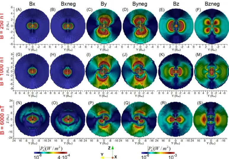
Figure3shows a view of the magnetic power from the night side of the exoplanet (PB(DS)) for different IMF orientations
Fig. 3.View of the magnetic power from the night side of the exoplanet for different IMF orientations and exoplanet intrinsic magnetic field intensities. The first color bar is related to the Bx–Bxneg IMF orientations, and the second color bar is related to the other IMF orientation. The plotted surface is defined between the bow shock and the magnetopause where the magnetic power reaches its maxima.
and exoplanet intrinsic magnetic field intensities. The minima of the magnetic power are correlated with a local decrease in the exoplanet magnetic field intensity, while the maxima are correlated with a local enhancement of the exoplanet magnetic field (pile up). The hot spot distribution for the Bx–Bxneg IMF orientations is north–south asymmetric (panels 3A, B, G, H, N, and O) because there is reconnection region at the south (north) of the magnetosphere if the IMF is oriented in the Bx (Bxneg) direction. The hot spots are displaced northward for Bx IMF orientations and southward for Bxneg IMF orientations as the exoplanet magnetic field intensity increases because the reconnection regions are located farther away from the exoplanet surface (the magnetopause standoff distance increases). The hot spot distribution for the By–Byneg IMF orientations shows an east–west asymmetry also correlated with the location of the reconnection regions (panels 3C, D, I, J, P, and Q). If the exo-planet magnetic field intensity increases the hot spots sideways the magnetic axis are located farther away from the exoplanet, caused by the increase in the magnetopause standoff distance and the counterclockwise (co) rotation of the hot spots for the By (Byneg) IMF orientation. The reconnection regions for the Bz (panels E, K, and R) and Bzneg (panels 3F, M, and S) IMF orientations are located near the exoplanet poles and the equator, respectively. If the exoplanet magnetic field intensity increases the reconnection regions are located farther away from the poles (equatorial region), and the hot spot distribution is located closer
to the equatorial (polar) region. In summary, the hot spots are located farther away from the exoplanet surface as the magnetic field intensity increases. It should be noted that a larger SW dynamic pressure leads to a more compact magnetosphere on the exoplanet’s day side, so the hot spots will be located closer to the exoplanet surface. Consequently, the correct identification of the exoplanet magnetic field intensity requires an accu-rate identification of the host start SW dynamic pressure at the exoplanet orbit (a deviation larger than a 50% from the real value, particularly if the stellar wind pressure is large, will lead to incorrect results). Such information can be par-tially inferred analyzing the radio emission from the exo-planet’s night side because a strong radio emission is a sign of intense magnetotail stretching and high SW dynamic pressure (Varela et al. 2016b).
Figure4 shows a view of the kinetic power from the night side of the exoplanet (Pk(DS)) of B6000 model for different IMF
orientations. A local decrease (enhancement) in the magneto-spheric field is associated with a local enhancement (decrease) in Pk(DS) caused by the acceleration of the plasma in the
recon-nection regions where the stellar wind is injected in the inner magnetosphere. Consequently, the Pk(DS) distribution is
deter-mined by the magnetosphere topology and IMF orientation. An increase of the SW dynamic pressure enhances the magnetic and kinetic powers, although the hot spot distribution is only slightly disturbed (Varela et al. 2016e).
Fig. 4.View of the kinetic power from the night side of the exoplanet in the B6000 model for different IMF orientations. The plotted surface is defined between the bow shock and the magnetopause where the kinetic power reaches its maxima.
Fig. 5. Magnetic power on the exoplanet’s night side (PB(NS)) for model B250 for Bx (panel A), By (panel B), and Bnegz (panel C) IMF orientations. The reconnection region (isosurface with magnetic field intensity between 0 and 20 nT) is indicated in dark blue and dark green; the magnetotail reconnection region is indicated by the yellow rectangle. Magnetic field lines of the exoplanet and IMF are indicated in red.
Figure 5 shows a zoomed view of the magnetic power (PB(NS)) on the night side for an exoplanet with a magnetic field
intensity of 250 nT for Bx, By, and Bzneg IMF orientations. The different IMF orientations modify the exoplanet’s magne-tosphere topology (red magnetic field lines) and reconnection regions between the exoplanet magnetic field and the IMF (dark blue and dark green iso-surfaces linked to the magnetopause and the magnetotail X point). For this reason, the location and inten-sity of the radio emission hot spots are different in each model. The last closed magnetic field line indicates the location of the magnetopause and the open magnetic field lines are reconnected lines between the IMF and the exoplanet magnetic field.
The expected radio emission is calculated from the net mag-netic and kimag-netic power dissipated on the planet’s day and night sides using the radiometric Bode law (Farrell 1999;Zarka et al. 2001) for different exoplanet magnetic field intensities:
[P(DS)]= a[Pk(DS)]+ b[PB(DS)], (7)
[P(NS)]= a[Pk(NS)]+ b[PB(NS)], (8)
with a and b the efficiency ratios assuming a linear depen-dency of [Pk] and [PB] with [P]. The radio emission measured
from the solar system planets can be explained by two possible combinations of efficiency ratios: (a= 10−5, b= 0) or (a = 0,
b= 2 × 10⁻³;Zarka 2007,2017). In the following, we only con-sider the combination of parameters a= 0, b = 2 × 10⁻³because the other combination leads to a radio emission several orders of magnitude smaller on the day and night sides. All the [P(DS)] and [P(NS)] values are calculated for an exoplanet with the same radius as Mercury (Rex = 2440) km to have a straightforward
comparison with the Varela et al. (2016e) results. The model is in adimensional units and the distance is normalized to the exoplanet radius, so [P(DS)] and [P(NS)] can be expressed in terms of any exoplanet radius considering that [W] = kg m2s−3.
For example, if we calculate the radio emission of an exoplanet with the same radius as the Earth, the values in the tables must be multiplied by a factor (REarth/RMercury)2 = 6.67. It should be
noted that the radius of the obstacle in the analysis of the radio emission is the distance from the magnetopause to the exoplanet surface, not the exoplanet radius; the radio power is enhanced as the module of the exoplanet magnetic field increases because the magnetosphere is wider. On the other hand, the ratio between the exoplanet radius must be included in the extrapolation to be con-sistent with the fact that the magnetic field module is compared at the exoplanet surface.
Table4shows the predicted radio emission on the exoplanet’s day side (top rows) and night side (middle rows). The radio emission increases with the magnetic field intensity, consistent with the theoretical scaling confirmed by the radio emission
Table 4. Kinetic power from the night side of the exoplanet for different IMF orientations (B6000 model).
[P(DS)] (105W)
Model Bx Bxneg By Byneg Bz Bzneg B250 0.63 0.63 6.90 8.72 5.96 11.3 B1000 2.18 2.04 12.4 12.2 10.6 29.5 B6000 4.34 4.21 35.0 32.5 14.7 72.5 Linear regression slope day side vs. Bex(1011W/T)
Bx Bxneg By Byneg Bz Bzneg α 0.77 0.74 6.05 5.65 2.71 12.6
∆α ±0.1 ±0.1 ±1 ±1 ±1 ±2
[P(NS)] (105W)
Model Bx Bxneg By Byneg Bz Bzneg B250 0.10 0.10 0.53 0.53 0.13 0.18 B1000 1.04 0.72 1.74 1.71 1.00 0.66 B6000 10.2 10.2 15.8 16.4 7.75 20.4
Linear regression slope night side (1011W/T)
Bx Bxneg By Byneg Bz Bzneg α 1.68 1.67 2.61 2.70 1.28 3.32 ∆α ±0.08 ±0.1 ±0.1 ±0.1 ±0.04 ±0.3
Notes. Expected radio emission on the exoplanet’s day side (first table) and in the magnetotail X point on the exoplanet’s night side (third table) for different IMF orientations (a= 0, b = 2 × 10⁻³) and exoplanet mag-netic field intensities. Slope (α) and goodness of fit (∆α) of the linear regression [P] = αBex for each IMF orientation (second and fourth table). Bexis the magnetic field intensity on the exoplanet surface and the exoplanet radius is Rex= 2440 km.
measurements of the gaseous planets in the solar system (Desch 1988; Zarka 2000, 2007; Zarka et al. 2001; Nichols & Milan 2016). It should be noted that the scaling law “emitted power” versus “impinging Poynting flux” only gives an order of magni-tude estimation for what may be observable with a given radio telescope, so the current paper is not about detection but about emission efficiency for various exoplanet magnetic field config-urations and stellar wind magnetic field orientations. In addition, the total radio power is integrated over all the frequencies of the emission although a radio telescope has a finite bandwidth, so the radio power in Table4overestimates the radio telescope measurements. The radio emission on the day side is almost one order of magnitude higher than the radio emission on the night side for all the IMF orientations in models B250 and B1000. On the other hand, the radio emission is larger on the night side in the model B6000 for the Bx–Bxneg IMF orientations. If we calculate the linear regression [P] = αBex (third table),
with Bexthe magnetic field intensity on the exoplanet surface,
we observe that only the IMF orientations Bx–Bxneg lead to a stronger radio emission on the night side. For the By–Byneg and Bz–Bzneg IMF orientations, the radio emission on the day side is two times larger than the night side. The fit goodness of the linear regression (∆α) shows a reasonable agreement with the data tendency. The radio emission on the night side of model B6000 shows a smaller variation between the different IMF ori-entations, because the internal magnetosphere topology is less affected by the IMF orientation as the exoplanet magnetic field
intensity increases. The strongest radio emission on the day side is observed for the Bzneg IMF orientation, followed by the By– Byneg orientations, whereas the Bx–Bxneg IMF orientations lead to the weakest radio emission. Thus, future radio emis-sion measurements require an observation time, long enough, to remove the effect of the IMF orientation (as well as the variation in the SW dynamic pressure) because the instantaneous radio emission can change by up to one order of magnitude if the IMF is oriented in the exoplanet–star, southward or northward orien-tations. Similar trends are reproduced in a previous study about the IMF effect on the Hermean magnetospheric radio emission (Varela et al. 2016e).
The maximum cyclotron frequency at the planetary surface for the models B250, B1000, and B6000 is fmax = 14, 56, and
336 kHz. Consequently, the radio emission from exoplanets with less than Bex ≈ 1000 nT is less likely to be observed (at least
for the stellar wind conditions analyzed in this article, where the plasma frequency is 69.5 kHz). Based on our knowledge at Jupiter, Saturn, and the Earth, the auroral radio emission (CMI) is produced between very low frequencies (kHz) and fmax. It
should be noted that the radio-magnetic scaling law relates the total power integrated on the emissions spectrum and beaming pattern (and average time variations). In addition, the average radio flux density can be deduced from the power divided by the spectral range (≈ fmax) and the solid angle in which the emission
is beamed (typically 0.2–1 sr; seeZarka & Cecconi 2004). The peak instantaneous flux density can exceed the average flux den-sity by 2 orders of magnitude (Galopeau et al. 1989; Zarka & Cecconi 2004;Lamy et al. 2008).
3.3. Effect of the magnetic field quadrupolar-to-dipolar components ratio
In this section we analyze the effect of the exoplanet magnetic field topology on the radio emission in configurations with dif-ferent ratios of the dipolar and quadrupolar components, namely, models Q02 (Bdip = 0.8 × Bex and Bquad = 0.2 × Bex nT)
and Q04 (Bdip = 0.6 × Bex and Bquad = 0.4 × Bex nT) with
Bex= 6000 nT, for different IMF orientations.
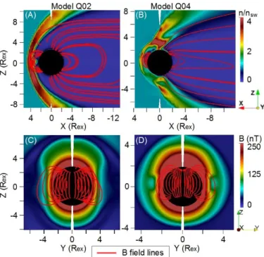
Figure6shows a polar cut of the density distribution (color scale, panels A and B) and the frontal plane of the magnetic field modulus (color scale, panels C and D) of the models Q02 and Q04 for a Bx IMF orientation. The red lines show the exoplanet magnetic field lines. Compared to the B6000 model, Q02 and Q04 modes show wider regions of open magnetic field lines on the planet surface and a smaller magnetopause standoff distance because an increase in the g20/g10 ratio leads
to the northward displacement and a faster decay of the exo-planet magnetic field. Consequently, the magnetosphere topol-ogy of the models Q02 and Q04 is different regarding the model B6000 so the reconnection regions, dissipation, and radio emission hot spot locations and intensity also change. More-over, a higher g20/g10 ratio leads to a thinner and deformed
magnetosheath, so the SW precipitates directly towards the exoplanet surface at low southern hemisphere latitudes in the Q4 model.
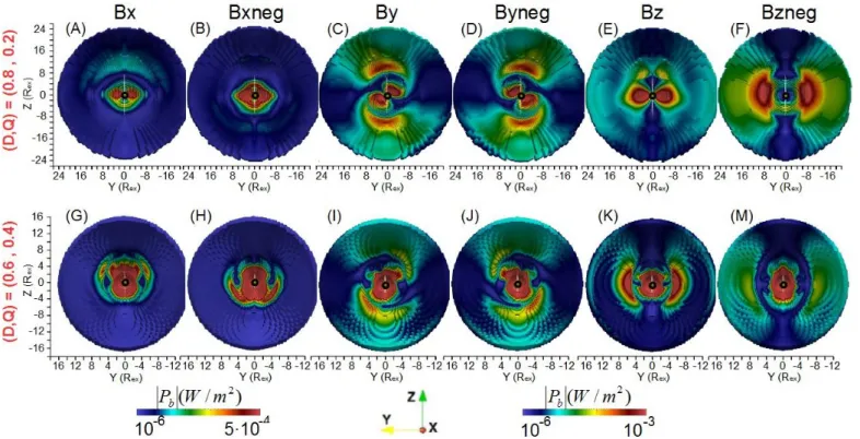
Figure7shows a view of the magnetic power from the night side of the exoplanet for different IMF orientations and exo-planet magnetic field topologies. If the IMF is oriented in the Bx–Bxneg directions (panels A, B, G, and H), an increment of the quadrupolar component of the exoplanet magnetic field leads to a northward drift of the hot spots, located farther away from the north pole for the Bx IMF orientation and closer to the equa-tor for the Bxneg IMF orientation regarding the B6000 model,
Fig. 6.Polar cut of the density distribution (color scale) and field lines of the exoplanet magnetic field (red lines) of models Q02 (panel A) and Q04 (panel B) for the Bx IMF orientation. The black disk radius is Rcr. Frontal cut of the magnetic field module on the star–exoplanet direction of models Q02 (panel C) and Q04 (panel D).
due to the northward displacement of the magnetosphere. A sim-ilar effect is observed for the By–Byneg IMF orientations (panels C, D, I and J) where the hot spots in the north of the magneto-sphere are located farther away from the exoplanet, although the hot spots in the south of the magnetosphere are located closer to the exoplanet. For the Bz–Bzneg IMF orientations, the hot spots are also displaced northward. The Q04 model shows for all the IMF orientations a region of large magnetic power near the exoplanet (panels K and M); compared to the B6000 and Q02 models (panels E and F), the magnetopause standoff distance is smaller and the reconnection regions are enhanced, which is caused by the strong deformation of the internal magnetospheric field compared to the dipolar case. These results point out that a northward displacement (or southward depending on the exo-planet magnetic field orientation) of the hot spot distribution, independently of the instantaneous IMF orientation, indicates a large quadrupolar component of the exoplanet magnetic field. It should be noted that the radio telescope observation angle with respect to the exoplanet and the exoplanet–host star vec-tor must be calculated accurately to avoid an overestimation of the quadrupolar component.
Figure8 shows the magnetic power (PB(NS)) on the
exo-planet’s night side and the magnetosphere topology of the model Q04 for the Bx, By, and Bz IMF orientations. Compared to the B6000 model (see Fig. 5) the magnetotail is slender and stretched, a consequence of a stronger perturbation of the inter-nal magnetosphere topology by the IMF due to a faster decay of the quadrupolar component with respect to the dipolar compo-nent, so the radio emission is lower. To quantify the magnetotail stretching, we calculate the ratio between the averaged width of the magnetotail with the location of the X point, showing values around 0.115 for the Bx IMF case, 0.169 for the By IMF case, and 0.187 for the Bz case, smaller than the B6000 model where the ratio for the Bx IMF case is 0.313 (2.7 times larger), for the
Table 5. Expected radio emission on the exoplanet’s day side for differ-ent IMF oridiffer-entations (a= 0, b = 2 × 10⁻³) and exoplanet magnetic field intensities.
[P(DS)] (105W)
Model Bx Bxneg By Byneg Bz Bzneg Q02 3.33 4.40 19.1 16.9 9.43 33.5 Q04 26.6 51.3 63.9 55.6 42.1 44.6
Model / B6000 [P(DS)] ratio
Model Bx Bxneg By Byneg Bz Bzneg Q02 0.77 1.05 0.55 0.52 0.64 0.46 Q04 6.13 12.2 1.83 1.71 2.86 0.61
Notes. Results for an exoplanet with a radius of Rex= 2440 km.
By IMF case is 0.399 (2.3 times larger), and for the Bz IMF case is 0.355 (1.9 times larger). Consequently, the radio emis-sion on the exoplanet’s night side varies almost by one order of magnitude between the different configurations.
Table5shows the expected radio emission for different ratios of the quadrupolar to dipolar components on the exoplanet’s day side (the values on the night side are not shown because the trends only indicate a decrease in the radio emission as the quadrupolar-to-dipolar ratio increases due to the faster decay of the quadrupolar component).
The radio emission of the model Q02 on the day side decreases for all the IMF orientations (except for the Bxneg case, which shows a slight increase) because the faster decay of the quadrupolar component leads to a weaker reconnection region showing similar internal magnetosphere topology than the B6000 model. If the quadrupolar component is large enough, as in model Q04, the internal magnetospheric topology changes with respect to the B6000 model leading to an enhancement of the reconnection regions and the radio emission near the exoplanet surface.
3.4. Effect of the exoplanet magnetic axis tilt
In this section we analyze the effect of the magnetic axis tilt on the exoplanet radio emission, namely the models tilt30 (tilt = 30◦), tilt60 (tilt = 60◦), and tilt90 (tilt = 90◦). The anal-ysis of the magnetic axis tilt is performed in addition to the study of the IMF orientation because different angles between magnetic axis and stellar wind velocity vector leads to different exoplanet magnetosphere configurations, due to the effect of the stellar wind dynamic pressure.
Figure9shows a view of the magnetic power from the night side of the exoplanet for different IMF orientations and exo-planet magnetic axis tilts. The hot spots distribution for the Bx (panels A and G) and Bxneg (panels B and H) IMF orientations are displaced respectively southward and northward as the tilt increases from 0◦ to 60◦ because the reconnection regions are displaced closer to (or farther away from) the star and closer to the exoplanet equatorial plane. In addition, models with a large tilt and a Bx (Bxneg) IMF orientation show a hot spot distri-bution similar to models with small tilt and a Bz (Bzneg) IMF orientation (compare panels N and O of Fig.4 with panels K, M, R, and S of Fig.9, or panels R and S of Fig.4with panels G and H of Fig.9). This comes about because the magnetosphere topology is almost analogous if the SW dynamic pressure is not
Fig. 7.View of the magnetic power from the night side of the exoplanet for different IMF orientations and exoplanet magnetic field topologies (different dipolar-to-quadrupolar component ratios). The first color bar is related to the Bx–Bxneg IMF orientations, and the second color bar is related to the other IMF orientations. The plotted surface is defined between the bow shock and the magnetopause where the magnetic power reaches its maxima.
Fig. 8.Magnetic power on the exoplanet’s night side (PB(NS)) of model Q04. The reconnection region (isosurface with magnetic field intensity between 0 and 20 nT) is indicated in dark blue and dark green; the magnetotail reconnection region is indicated by the yellow rectangle. Magnetic field lines of the exoplanet and IMF are indicated in red.
strong enough to drive major deformations on the magnetosheath structure. Compared to the B6000 model the hot spots are more spread out and located farther from the exoplanet by the effect of the SW dynamic pressure because as the tilt increases the IMF is more aligned with the SW flow. The model tilt90 has a recon-nection region in the exoplanet equatorial plane where the IMF and magnetic field lines are (anti-)parallel if the IMF is oriented in the Bx (Bxneg) direction. Thus, the SW precipitates directly towards the surface at the equator and there is an enhancement of the magnetic power near the exoplanet. The hot spot distribution is located in the region with closed magnetic field lines, forming a ring around the exoplanet in the XY plane. For the By–Byneg IMF orientations, the hot spots at the north of the magnetosphere are located farther away from the exoplanet and more aligned
with the magnetic axis as the magnetic axis tilt increases, so the east–west asymmetry of the magnetosphere decreases (panels C, D, I, J, P, and Q).
Figure10shows the magnetic power (PB(NS)) of the
mod-els tilt30, tilt60, and tilt90 on the planet’s night side for the Bx IMF orientation. The magnetotail topology changes as the tilt increases, showing a more slender and stretched shape, so the radio emission also changes for each configuration. The ratio between the magnetotail width and X point location is 0.232 for the Bx IMF tilt30 case, 0.212 for the Bx IMF tilt60 case, and 0.135 for the Bx IMF tilt90 case. Model tilt90 is an extreme case with a reconnection ring in the YZ plane due to the bending of the closed magnetic field lines by the SW at the north and south geographic poles towards the star–exoplanet direction.
Fig. 9.View of the magnetic power from the night side of the exoplanet for different IMF orientations and exoplanet magnetic axis tilts. The color bars of the model tilt90 for the Bx–Bxneg IMF orientations are different from those in the rest of the panels. The plotted surface is defined between the bow shock and the magnetopause where the magnetic power reaches its maxima.
Table 6 shows the radio emission for different magnetic axis tilts on the planet’s day side. Increasing the magnetic axis tilt from 0◦ to 60◦ leads to a stronger radio emission
for the Bx–Bxneg IMF orientations because the reconnection regions and hot spots are wider. On the other hand, if the tilt is 90◦, the radio emission for the Bx (Bxneg) IMF orientation decreases (increases) due to the increase (decrease) in the exo-planet magnetic field near the magnetic poles by the effect of the magnetic reconnections (see Fig.9). If the IMF is oriented in the By–Byneg IMF direction, the radio emission increases between 0◦ and 30◦ because the hot spots are wider, although from 30◦to 90◦ both radio emission and hot spot size saturate.
For the Bz–Bzneg IMF orientations, the radio emission and hot spot size decreases as the tilt increases. On the other hand, the radio emission and hot spot size increases in the model tilt90. On the exoplanet’s night side, the radio emission increases with the tilt because the magnetotail stretching is greater.
4. Discussion and conclusions
The aim and main contribution of the present communication is to show the radio emission as a potential tool for identifying the exoplanet’s magnetic field properties. The information provided will be useful to guide future radio emission measurements to infer the exoplanet’s magnetosphere properties such as the mag-netic field intensity, tilt angle, and topology for different IMF orientations.
The analysis shows that the energy dissipation, hot spot distribution, and total radio emission are correlated with the exoplanet magnetic field topology and IMF orientation. Differ-ent magnetospheric configurations lead to differDiffer-ent locations of the reconnection regions and hot spot distributions on the exoplanet’s day side, associated with the maximum of the mag-netic power and the minimum of the kimag-netic power, as well as local enhancements of the magnetospheric field. Therefore the characteristics of the exoplanet’s magnetic field could likely be inferred by future radio telescopes because the radio emission measurements contain information about the exoplanet’s mag-netic field intensity, dipolar-to-quadrupolar components ratio, and magnetic axis tilt. The present and planned low-frequency radio telescopes with high sensitivity will reach 0.1–1 angu-lar resolution, enough to separate an exoplanet from a star if the exoplanet orbits at several AU and the system is not farther than a few tens of parsecs, but will unlikely resolve structures within the exoplanetary magnetosphere. On the other hand, from the modeling of the dynamic spectrum in intensity and circular polarization, it is possible to deduce several physical parameters from the system, including the planets magnetic field amplitude, tilt, offset, planetary rotation period, or the inclination of the orbital plane (Hess & Zarka 2011).
An increase in the exoplanet magnetic field intensity leads to an enhancement of the radio emission on the exoplanet’s day and night sides, and to an increase in the hot spot size located farther away from the exoplanet surface (Fig.11A). A linear regression between the exoplanet magnetic field and the radio emission on
Fig. 10.Magnetic power on the exoplanet’s night side (PB(NS)) of models tilt30, tilt60, and tilt90 for the Bx IMF orientation. Panels G and H show models tilt30 and tilt90 for a Bx IMF orientation. The reconnection region (isosurface with magnetic field intensity between 0 and 20 nT) is indicated in dark blue and dark green; the magnetotail reconnection region is indicated by the yellow rectangle. Magnetic field lines of the exoplanet and IMF are indicated in red.
the day and night sides also shows a reasonable agreement. In addition, a large quadrupolar component of the exoplanet mag-netic field leads to a northward (or southward) displacement of the magnetospheric field and the hot spot distribution. If the quadrupolar component is large enough (g20/g10 > 2/3), the
internal magnetospheric field is deformed compared to a pure dipolar case, leading to a larger radio emission on the exoplanet’s day side (Fig.11, panel C), although the radio emission on the night side decreases due to the faster decay of the quadrupolar component compared to the dipolar component.
The models with a small tilt and a Bx (Bxneg) IMF orien-tation have a similar magnetospheric topology to configurations with large tilt and Bz (Bzneg) IMF orientation (and vice versa), although not the same because the angle between the magnetic axis and stellar wind velocity vector is different. The magne-tosphere topology can be different if the stellar wind dynamic pressure is large enough to drive strong deformations on the magnetosheath, for example, if the host star has strong stellar wind fluxes or the exoplanet is in an orbit close to the host star. The consequence is an enhancement of the radio emission on the day side as the tilt increases for the Bx–Bxneg IMF orientations and a decrease for the Bz–Bzneg IMF orientations (Fig. 11D). On the other hand, if the exoplanet magnetic axis tilt is large the hot spot distribution is more spread out due to the effect of the SW dynamic pressure, because the SW is more aligned with the magnetic poles leading to an increase in the radio emission.
The radio emission on the night side is dominant for the Bx–Bxneg IMF orientations if the exoplanet magnetic field intensity is higher than 1000 nT, although the radio emis-sion on the day side is larger for the other IMF orientations
(Fig.11, panel B). If we extrapolate the trends obtained for the radio emission and exoplanet magnetic field intensity on the day and night sides (using the stellar wind parameters listed in Table3), the expected radio emission range of a hot Jupiter with Bex = 5 × 10⁵ nT and a radius of Rex = 7.2 × 10⁴ km
(simi-lar to Jupiter) is [P(DS)]= 0.3 − 5.5 × 10¹¹W and [P(NS)]=
0.7 − 1.4 × 10¹¹W and of a super Earth with B
ex= 6 × 10⁴ nT
and Rex = 1.26 × 10⁴ km is [P(DS)]= 0.6 − 9.6 × 10⁸ W and
[P(NS)]= 1.3 − 2.5 × 10⁸ W, values consistent with the
obser-vational scaling (Desch & Kaiser 1984;Zarka 1992;Zarka et al. 2001;Nichols & Milan 2016). Previous numerical studies pre-dicted the radio emission of a hot Jupiter located 3–10 radius away from a star similar to the Sun (Nichols & Milan 2016), suggesting a value of [5, 1300]1012W for an exoplanet magnetic
fields between 0.1 and 10 times Jupiter’s magnetic field, several orders of magnitude above the present model expectations. The reason for this difference is the dynamic pressure, almost 3 × 10³ times lower in the present model. As a proxy of the magnetic power enhancement with the increase in the dynamic, pressure, we consider the results ofVarela et al.(2016e): a dynamic pres-sure 3000 times higher leads to a radio emission enhancement of 2700 times with respect to the present model. This means that the expected maximum magnetic power of the model is [PB(DS)] ≈ 1.5 × 10¹⁸ W and [PB(NS)] ≈ 0.4 × 10¹⁸ W,
simi-lar to the analysis performed bySaur et al.(2013) andStrugarek et al.(2015), who expected a magnetic power around 1019W. For the same reason, the observational scaling shows a radio emis-sion value almost one order of magnitude higher than the Jupiter radio emission measurements because the dynamic pressure at the Jupiter orbit is lower. Nevertheless, the real radio emission
Table 6. Expected radio emission on the exoplanet’s day and night sides for different IMF orientations (a= 0, b = 2 × 10⁻³) and magnetic axis tilts.
[P(DS)] (105W)
Model Bx Bxneg By Byneg Bz Bzneg tilt30 55.1 19.6 87.3 80.1 7.36 49.9 tilt60 74.6 32.4 81.5 82.0 2.94 4.06 tilt90 18.7 57.6 10.8 7.87 19.1 60.1
Model / B6000 [P(DS)] ratio
Model Bx Bxneg By Byneg Bz Bzneg tilt30 12.7 6.66 2.49 2.46 0.5 0.69 tilt60 17.2 7.70 2.33 2.52 0.20 0.06 tilt90 4.34 13.7 0.31 0.24 1.30 0.83
[P(NS)] (105W)
Model Bx Bxneg By Byneg Bz Bzneg tilt30 70.7 72.8 95 108 48.9 108 tilt60 98.3 89.8 114 119 62.1 192
XModel / B6000 [P(NS)] ratio
Model Bx Bxneg By Byneg Bz Bzneg tilt30 6.93 7.14 6.01 6.59 6.31 5.29 tilt60 9.64 8.80 7.21 7.26 8.01 9.41
Notes. Results for an exoplanet with a radius of Rex= 2440 km.
must be larger in a hot Jupiter with respect to the present results because we do not add the effect of other radio emission sources such as the fast rotation or internal plasma releases that do not depend on the distance to the parent star, thus the extrapolation result may be considered as a lower bound. If the hot Jupiter is located at 20 parsec, the radio emission flux at Earth can be cal-culated asΦ = P/Ωd2ω with Ω ≈ 1.6 sr the solid angle, d the
distance to the exoplanet, and ω= 15 MHz the detection band-width of the receiver, leading to a value of 0.1−1 mJy, in the limit of the LOFAR observation range. For the case of a super Earth Φ ≤ 10−4mJy. The radio emission flux is lower than 10−4mJy in
the simulations performed in our study (e.g., model B6000 with a Bzneg IMF orientation,Φ = 3 × 10⁻⁵mJy), although stronger wind conditions lead to a higher radio emission flux. In addition, the model is only representative of an exoplanet with dipolar field without magnetic axis tilt in an orbit similar to Mercury for a host star like the Sun. If the exoplanet is located closer to the host star the SW dynamic pressure and IMF intensity is higher so the radio emission is also enhanced. Likewise, if the host star magnetic activity is higher the IMF is also larger (stars younger than the Sun with faster rotation are more active; see, e.g.,Emeriau-Viard & Brun 2017) as well as the radio emission. The SW and IMF characteristics also change if the host star is not the same type as the Sun, leading to a different scaling (Réville et al. 2016). In other words, dedicated analyses are required to foresee the threshold of the exoplanet magnetic field topology for each star spectral type, age, magnetic activity, and exoplanet orbital distance (Jardine & Collier Cameron 2008;Vidotto et al. 2010,2012;See et al. 2015;Weber et al. 2017).
The radio emission in models with different IMF orientation show a variability factor up to 20, describing how the radio emis-sion of an exoplanet should change during the magnetic cycle
of the host star or through IMF variations along the exoplanet orbit (Vidotto et al. 2011a). Such variability can partially explain the uncertainty in the determination of the average auroral radio powers using the radio Bode law, around one order of magnitude between the lower and upper bounds (Zarka et al. 2001).
The radio emission can escape the exoplanet magnetosphere if the maximum CMI emission is larger than the plasma fre-quency in the surrounding stellar wind. In the case of Mercury, the maximum CMI emission probably does not exceed a few 10s kHz, whereas the plasma frequency in the surrounding solar wind is between 70 and 100 kHz, thus the CMI radiation–if it exists (which should be confirmed by BepiColombo and MMO measurements) – is trapped in the magnetospheric cavity. For close-in exoplanets, if the planets exo-ionosphere is expand-ing the CMI emission can be trapped inside the magnetosphere (Weber et al. 2017), although there are several possibilities for overcoming the CMI emission trapping; for example, if the exoplanet shows small-scale auroral plasma cavities like at the Earth, there are second harmonic emissions (especially on the ordinary mode) or if the exoplanet magnetic field is strong. Another option is to analyze the radio emission from exoplan-ets located farther away from the host star where the plasma frequency is lower.
Using the results of the present study, it is possible to iden-tify, in a first approximation, the minimum exoplanet radio emission associated with a magnetic field strong enough to shield the exoplanet surface (at low latitudes) from the stel-lar wind. The exoplanet magnetopause standoff distance can be estimated by this simplified expression:
RMP Rex = B2 ex mpnµ0v2 !1/6
Here RMPis the magnetopause standoff distance and mpthe
pro-ton mass (we consider the same SW dynamic pressure as in the simulations; see Table3). If the ratio is RMP/Rex = 1, the SW
precipitates directly toward the exoplanet surface, so the mag-netic field is not strong enough to shield the planet, namely, Bex≈ 120 nT. If the exoplanet has the same radius as the Earth
and the magnetic field is a dipole without magnetic axis tilt, the radio emission range is [P(DS)] = 0.6−10 × 105 W and
[P(NS)]= 1.3−2.7 × 10⁵ W, so we can identify a threshold for the exoplanet habitability from the point of view of the radio emission output: if the radio emission measurement is lower than [P]= 106W, the exoplanet is less likely to host life on the surface (Vidotto et al. 2011b,2013). There are other restrictions for the exoplanet habitability, for example, the host star age. If the star is younger than the Sun, the magnetic activity is higher, due to a faster rotation, so extreme events such as the coronal mass ejec-tions (CME) are more frequent (Aarnio et al. 2012), which is why the exoplanet habitability requires a stronger magnetic field with a larger magnetopause standoff distance (Khodachenko et al. 2007;Lammer et al. 2007). If RMP/Rex= 5, the exoplanet surface
will be also shielded from most of the CME, so the exoplanet magnetic field must be at least Bex ≈ 1.5 × 10⁴ nT, leading to
a radio emission of [P(DS)]= 0.7−13 × 107 W and [P(NS)]= 1.7−3.3 × 10⁷ W. Thus, we can define another radio emission
threshold for exoplanet habitability of [P] = 1.3 × 10⁸ W if the host star is younger and more active than the Sun (but the same star type). Compared to the case of the Earth (older host star with lower SW dynamic pressure and IMF intensity at the exoplanet orbit), previous studies indicate a radio emission of at least 107W for a magnetosphere that can host life on the surface (Zarka 1998), a value compatible with the present results.
It should be noted that the expression to calculate the stand-off distance only provides an approximated value, because a dipolar magnetic field with no tilt is assumed and the effect of the IMF orientation is not considered, so dedicated numerical experiments are required to obtain more accurate thresholds. In addition, these results are only valid if the SW dynamic pressure and IMF intensity at the exoplanet orbit are similar to the case of Mercury.
The combination of efficiency ratios (a= 0, b = 2 × 10⁻³) shows the highest radio emission values. A previous study of the radio emission from the Hermean magnetosphere identified these efficiency ratios as the most accurate option for reproduc-ing the expected radio emission from Mercury (Varela et al. 2016e), but these results should be confirmed by in situ mea-surement and radio emission data from gaseous planets of the solar system. The present study’s results can also be used to compare the expect radio emission of Bode’s law with radio tele-scope measurements, with the aim of inferring the efficiency ratios that most closely fit the observations for different SW dynamic pressures, IMF orientations, and planet magnetic field topologies.
The trends obtained in the analysis are useful for the exo-planet magnetospheres detectable by the current radio tele-scopes, particularly hot Jupiters. Among other conclusions, we show that the present radio telescopes have enough sensitivity to measure the hot Jupiter radio emission, and in the best cases can possibly even constrain their magnetic field topology. In addi-tion, the model can be calibrated analyzing the radio emission from the gaseous planets of the solar system – the results of the analysis and the scaling are similar to these measurements and to models of other authors – and in the near future by the measure-ment of the radio emission from Mercury by the BEPIColombo satellite.
The net magnetic energy dissipation predicted by Bode’s law and the simulations show good agreement, so the mag-netic energy dissipation on the day side and the magnetotail reconnection regions are well reproduced by the model in a first approximation. On the other hand, the net kinetic energy dissi-pation predicted by the simulations is smaller than calculated by Bode’s law because the model can reproduce more accurately the complex flows on the day and night sides of the exoplanet.
Future measurements of the radio emission will allow testing of the different configurations of the exoplanet magnetospheres in the light of the model selection problem in Bayesian statistics (William 2016). In other words, it will be possible to select the model that best reproduces the observations based on the compu-tation of the Bayesian evidence (Trotta 2008;Corsaro et al. 2013; Corsaro & De Ridder 2014), a key parameter that provides a sta-tistical weight, favoring models that provide a better fit to the data but penalizing those that have a more complex analytical representation, i.e., a larger number of parameters that configure the model itself. In this way it will be possible to unambiguously constrain the most favored theoretical interpretation for a given observational set.
In summary, radio emission data bring constraints on the exoplanet magnetosphere topology, essential information to fore-see the potential habitability of exoplanets, associated with the presence of permanent and strong enough magnetic fields to shield the planet surface and atmosphere from the stellar wind erosion. This information can be deduced if we analyze large time series of radio emission data when available (Hess & Zarka 2011;Zarka et al. 2015), removing the effect of the instantaneous effect of the IMF orientation, intensity, and the stellar wind
Fig. 11.Panel A: radio emission on the day side vs. exoplanet magnetic field intensity. Panel B: radio emission on the night side vs. the exo-planet magnetic field intensity. Panel C: radio emission on the day side vs. the ratio of the exoplanet quadrupolar to dipolar magnetic field com-ponents. Panel D: radio emission on the day side vs. the magnetic axis tilt. Results for an exoplanet with a radius of Rex= 2440 km.
dynamic pressure and temperature. On the other hand, after iden-tifying the characteristics of the exoplanet magnetic field, the radio emission data is useful in order to determine the properties of the stellar wind and magnetic field of the star. This process can be carried out through the adoption of a Bayesian model compar-ison. In this view, the competing models to test will incorporate the different configurations of the exoplanet magnetospheres, as shown in this work, and will be fit to the radio emission data in order to obtain the best set of free parameters which best match the observed radio emission. In a subsequent step, the Bayesian evidence of each model are compared in order to select the most likely configuration that reproduces the same observa-tional set (Corsaro & De Ridder 2014). Our aim is to develop this thorough statistical approach by computing a grid of predictive models for future releases of radio emission measurements, and to test the methodology using synthetic datasets. The final tar-get is to create a catalog that illustrates the main features of the exoplanets’ magnetic fields and identify those that can harbor life.
Acknowledgements.This material is based on work supported by both the U.S. Department of Energy and the Office of Science, under Contract DE-AC05-00OR22725 with UT-Battelle, LLC. The research leading to these results has received funding from the European Commission’s Seventh Frame-work Programme (FP7/2007-2013) under the grant agreement SHOCK (project No. 284515), the grant agreement SPACEINN (project No. 312844), and ERC STARS2 (207430). We extend our thanks to CNES for Solar Orbiter and PLATO science support and to INSU/PNST for our grant. We acknowledge GENCI allocation 1623 for access to the supercomputer where most of the simula-tions were run, and DIM-ACAV for supporting the ANAIS project and our graphics/post-analysis and storage servers, as well as DIO of the Paris Obser-vatory. The authors would also like to acknowledge R.A. Garcia and E. Corsaro for the fruitful discussion. This manuscript has been authored by UT-Battelle, LLC under Contract No. DE-AC05- 00OR22725 with the U.S. Department of Energy. The US Government retains and the publisher, by accepting the article for publication, acknowledges that the US Government retains a non-exclusive, paid-up, irrevocable, worldwide license to publish or reproduce the published form of this manuscript, or allow others to do so, for US Government pur-poses. The Department of Energy will provide public access to these results of federally sponsored research in accordance with the DOE Public Access Plan