HAL Id: halshs-00749500
https://halshs.archives-ouvertes.fr/halshs-00749500
Preprint submitted on 7 Nov 2012
HAL is a multi-disciplinary open access archive for the deposit and dissemination of sci-entific research documents, whether they are pub-lished or not. The documents may come from teaching and research institutions in France or
L’archive ouverte pluridisciplinaire HAL, est destinée au dépôt et à la diffusion de documents scientifiques de niveau recherche, publiés ou non, émanant des établissements d’enseignement et de recherche français ou étrangers, des laboratoires
Ambiguity and Coordination in a Global. Game Model
of Financial Crises
Daniel Laskar
To cite this version:
Daniel Laskar. Ambiguity and Coordination in a Global. Game Model of Financial Crises. 2012. �halshs-00749500�
WORKING PAPER N° 2012 – 40
Ambiguity and Coordination in a Global
Game Model of Financial Crises
Daniel Laskar
JEL Codes : D81, D82, G01
Keywords: Financial crises ; Ambiguity ; Uncertainty ; Global games ; Coordination ; Transparency
P
ARIS-
JOURDANS
CIENCESE
CONOMIQUES48, BD JOURDAN – E.N.S. – 75014 PARIS TÉL. : 33(0) 1 43 13 63 00 – FAX : 33 (0) 1 43 13 63 10
Ambiguity and Coordination in a Global
Game Model of Financial Crises
Daniel Laskar
∗November 6, 2012
Abstract
We consider a two-player global game where creditors, who finance some investment project, have to decide whether to roll over their loans or not. We use a non-Bayesian approach where creditors exhibit some aversion to ambiguity. We show that an increase in ambiguity reduces the perceived coordination of players in rolling over their loans. This contibutes to increasing the probability of a financial crisis, and therefore provides an additional argument in favor of transparency in the model considered.
JEL classification: D81; D82; G01.
Keywords: financial crises; ambiguity; uncertainty; global games; coordination; transparency.
1
Introduction
The literature on financial crises has underlined that, besides the underlying state of the economy (the strength of fundamentals), the interdependence between the decisions of the participants in the financial markets may play a crucial role. These decisions may exhibit some complementarities. For example, the possibility of a bank run depends on the amount of depositors who withdraw their money deposited at the bank. In the same way, a cur-rency crisis requires that a sufficient amount of speculators go against the currency. Also, when a group of creditors finance some investment project,
∗Paris School of Economics-CNRS, France. Address: CEPREMAP, 142 rue du
Chevaleret, 75013 Paris, France. Ph: 33 (0)1 40 77 84 08. Fax: 33 (0)1 40 77 84 00. E-mail: daniel.laskar@ens.fr
a financial crisis, due to an early liquidation by creditors, occurs only when an insufficient amount of creditors roll over their loans.
As it has been shown in the literature, the presence of these comple-mentarities between the decisions of economic agents may lead to multiple equilibria. Thus, if each one expects that other depositors withdraw their money deposited at the bank, then a bank run will occur. But such a bank run would not have occurred if, on the contrary each depositor did not expect other depositors to withdraw their money. Concerning currency crises, for some range of the values of fundamentals, a currency crisis would occur if everyone expected other participants to attack the currency, but the crisis would not occur if, on the contrary, each one expected that other partici-pants do not attack the currency. Similarly, for some range of fundamentals, an investment failure due to an early liquidation by creditors would occur if each creditor expected that other creditors do not roll over their loans, but there would be no failure if each creditor expected that other creditors roll over their loans. In each case, the corresponding game has an equilibrium with a financial crisis, and an other one without a financial crisis1.
These models which lead to multiple equilibria assume that the decision makers know the relevant state variable. However, when market participants only receive imprecise signals on the relevant state variable, the literature has shown that the multiplicity of the game disappears and that a unique equilibrium emerges. In such a class of games, called "global games" in the literature2, where we only have one equilibrium, it becomes meaningful to do
comparative statics exercises where we study the effect of changes in some exogenous parameters of the model. Furthemore, as some uncertainty is in-troduced in the model through the imprecision of signals, one can try to examine how the amount of uncertainty affects the equilibrium. Thus, it be-come possible to ask whether more uncertainty increases the probability of a financial crisis or not. According to the existing literature, the comparative statics exercises done with these models lead to ambiguous results. Depend-ing on the parameters of the model, greater uncertainty may either increase or decrease the probability of a crisis3.
These results of the literature are obtained under the usual Bayesian approach to uncertainty, where each decision maker holds some prior prob-ability distribution on unknown parameters and maximizes expected utility. However, this Bayesian approach to uncertainty has been challenged. Knight (1921) had already made the distinction between a situation of "risk" where
1See Diamond and Dybvig ((1983) and Obstfeld (1996) for such analyses.
2See Carlson, H. and E. van Damme (1993) and, for a survey on global games, see
Morris and Shin (2003) .
there is a known probability distribution, and a situation of "(Knightian) un-certainty" where no known probability distribution exists. Ellsberg (1961), through some experiments, has shown that decision makers exhibit some "aversion to ambiguity". They prefer a situation where there is a known probability distribution to a situation where this distribution is unknown. This is why, in the last two or three decades, some new non-Bayesian ap-proaches to uncertainty, where such an aversion to ambiguity could be taken into account, have been developped4.
Such a non Bayesian approach has been applied to a large variety of issues in economics. It has been shown that this approach could help explain some stylized facts, and could allow us to better understand some results which otherwise looked quite paradoxical5. It would therefore be worthwhile to try to apply this approach to the issue of financial crises, and more particularly to the global game models of crises.
In fact, recently, Ui (2009) has introduced such a non-Bayesian analysis in the context of global games. When applied to some standard global games models of financial crises, Ui (2009) has underlined that the effect of ambi-guity may depend on the kind of model considered. Thus, in a global game model of currency attacks (as in Morris and Shin (1998)), more ambiguity appears to have a favorable role: more ambiguity tends to prevent a cur-rency attack to occur. On the contrary, in a global game model of bank runs (Goldstein and Pauzner (2005)), ambiguity has a detrimental effect: more ambiguity increases the probability of a bank run. Kawagoe and Ui (2010) have considered ambiguity in a two player version of a global game model where some creditors have to decide whether to roll over their loan or not for some investment project (as in Morris and Shin (2004)). They show that more ambiguity has a detrimental effect: it increases the probability that the players do not roll over their loans6.
4Two classical references are Gilboa and Schmeidler (1989) and Schmeidler (1989).
In these non-Bayesian frameworks, the presence of some aversion to ambiguity leads the decision maker to give more weight to the bad outcomes implied by each decision.
5On the application of such a non Bayesian approach to various issues, and on how this
approach may help explain some existing empirical puzzles, see for example Mukerji and Tallon (2004).
6As explained in Ui (2009), the reason for having these different effects of ambiguity
is the following. More ambiguity makes players more willing to choose the action with a payoff which does not depend on the unknown state of fundamentals. In the bank runs model, and in the model of coordination of creditors to roll over their loans, this action helps the crisis to occur. It respectively consists in withdrawing the deposits (and then getting cash), or in not rolling over the debt (and then getting the known value of the collateral). On the contrary, in the currency attacks model, it is the action which consists in not attacking the currency, i.e. in not participating to the creation of the crisis, which
In this paper, we will pursue this kind of analysis. We will underline that the analyses of Ui (2009) and Kawagoe and Ui (2010) actually do not give full scope to the role of ambiguity in global models of financial crises. They do not underline the role that ambiguity may have on the issue of the perceived coordination of the players, i.e. on the belief that each player has on the coordination of players. But this is crucial because of the complemen-tarities involved. As we will emphasize, ambiguity creates a gap between the belief that each player holds on the probability distribution of the signal she receives, on the one hand, and the belief that each player holds on the prob-ability distributions of the signals that other players receive, on the other hand. Such a difference was not allowed in the analyses of Ui (2009) and Kawagoe and Ui (2010) because it was a priori assumed that the probability distributions of the signals received by all the players were identical. In the present paper, by relaxing this assumption, we are able to underline that ambiguity may have an adverse effect on the perceived degre of coordination of the players which is held by each player.
We will use a model close to the model considered in Kawagoe and Ui (2010), which is itself inspired by Morris and Shin (2004). It is a two-player global game between two creditors who finance some investment project. At an interim stage, each player has to decide whether to roll over her loan or not.
We will show that more ambiguity decreases the degree of coordination of players which is perceived by each player when he considers rolling over her loan. This will make each player less willing to roll over the loan, and therefore makes a crisis more likely. Thus, our analysis will highlight an additional channel through which ambiguity can precipitate a financial crisis. This will reinforce the argument found in the literature that ambiguity plays a detrimental role in financial crises in such a model. As more transparency from the public authorities may reduce the amount of ambiguity that each player has to face, our results will make the case for transparency stronger in this model.
The model is presented in Section 2. Section 3 derives the equilibrium of the game. Section 4 considers the effect of more ambiguity. Section 5 concludes.
2
Model
As in the global game model of Morris and Shin (2004), a group of creditors are financing some investment project through some collaterized debt. At
some interim stage, each creditor can either roll over the loan until the ma-turity of the investment project, or seize the collateral, which has some given known value λ. The value of the investment project at maturity will depend on the state of fundamentals, represented by some real variable θ. The value of fundamentals θ is not known to creditors, but each creditor receives an imperfect signal on θ. The value of the investment project at maturity will also be negatively affected if an insufficient amount of creditors do not roll over the debt. This creates some complementarities between the decisions of creditors to roll over the debt or not. The model considers the corresponding game between the creditors. As in Kawagoe and Ui (2010), we will consider a two-player version of the game, and we will introduce some ambiguity (or "Knightian uncertainty") on θ with ambiguity adverse players7.
The actions and payoffs of this two-player game are the following. Each player has two possible actions: to roll over the loan (R), or not to roll over the loan (N). By choosing N, the player receives the value of the collateral λ, where λ satisfies the inequality 0 < λ < 1. By choosing to roll over the loan (R), a player gets a payoff equal to 1 when the investment project succeeds, and a payoff equal to 0 when the investment project fails. It is assumed that the investment project always succeeds when the fundamentals are good enough, i.e. when we have θ > 1; and that the project always fails when the fundamentals are bad enough, i.e. when we have θ < 0. For intermediate values of the fundamentals, i.e. in the case 0 ≤ θ ≤ 1, it is assumed that the investment project succeeds only in the case where both players roll over the loan. The payoff matrix in the case 0 ≤ θ ≤ 1 (which is the case where the coordination of players matters) is therefore:
R N
R 1, 1 0, λ N λ, 0 λ, λ
If the value of θ was known to the two players, then, in the case θ > 1, R would be a dominant strategy; while in the case θ < 0, N would be a dominant strategy. In the case 0 ≤ θ ≤ 1, there would however be two equilibria: a bad financial crisis equilibrium (N,N), where no player rolls over the loan and where, consequently, the inverstment project fails; and a good equilibrium without a financial crisis (R,R), where each player rolls over the loan, and where, as a consequence, the investment project succeeds.
Here, however, as in the global game literature, it is assumed that θ is
7Ui (2009) introduces the same kind of ambiguity in a more general global game with
not known to the players. Each player receives a signal xi given by
xi = θ + ξi (1)
where ξi is a random variable.
In the literature on global games, it is usually assumed that ξi follows some given known probability distribution. It can be shown that, when we have 0 ≤ θ ≤ 1, then there is a unique equilibrium instead of the two equilibria which would have been obtained if θ was known. This occurs even when the uncertainty becomes small, i.e. when the variance of ξi goes to
zero8.
Here, the assumption that the probability distribution of ξi is known will be removed and it will be assumed that there is (Knightian) uncertainty, or "ambiguity", on some parameter underlying the distribution of ξi. As
indi-cated before, Ui (2009) and Kawagoe and Ui (2010) considered an analysis of the effect of ambiguity in global games. They assumed that ξi followed some
distribution but that the variance σ of this distribution was unkown. There was some ambiguity on the value of this variance. Each player was assumed to maximise the minimum of the expected utility, where the minimum is taken for σ belonging to some interval [σ, σ].
The crucial difference between our analysis and the analyses of Ui (2009) and Kawagoe and Ui (2010) is the following. In Ui (2009) and Kawagoe and Ui (2010), it is assumed that the probability distributions of the signal are the same for all the players. Here, we will remove such an assumption. For, each player may not necessarily get the same kind of information and may interpret an information in a different and personal way. This could change not only the signal received but also the underlying probability distribution of the signal. Thus, if there is some uncertainty on the probability distri-bution underlying the signal received by each player, it seems restrictive to assume that the same probability distribution underlies the signals received by all the players. It would therefore be worthwhile to consider what happens if we allow the signal received by each player to follow a probability distri-bution which may not be the same for all the players. This is what we will consider in our analysis. As we will see, this will permit ambiguity to have a stronger effect, because of its consequences on the perceived coordination of the players
To simplify the analysis we will also assume that it is the mean (rather
8In that case, although each player would be almost certain about the value θ of the
fundamentals, there would remain a non negligible uncertainty on higher orders beliefs. This is sufficient to produce a unique equilibrium. See Morris and Shin (2003) for a review of these kinds of models.
than the variance) of the probability distribution of ξi which is uncertain9.
Thus player i receives a signal with a possible "bias" µi, which is assumed to be uncertain10. We will write
ξi = µi+ εi (2)
where εi is a zero-mean random variable which has a known probability
distribution, and where the mean µi of ξi depends on i, and therefore is not
necessarily the same for the two players. The random variables ε1 and ε2 are
assumed to be stochastically independent. We therefore have
xi = θ + µi + εi (3)
There is ambiguity on the value of the mean (or "bias") µi . We will assume that each µi, i = 1, 2, belongs to the interval
£
µ, µ¤ and that each player has a corresponding maxmin criterion of expected utility11. We allow
the distributions of the signals received by the players to be different, by allowing µ1 6= µ2.
As in Kawagoe and Ui (2010), we assume that θ is uniformally distributed on [−δ, 1 + δ] , with δ > 0; and that εi is uniformally distributed on [−γ, γ] .
9Because we remove the simplifying assumption that the signals received by the players
may not follow the same probability distribution, we have chosen to take the mean of the probability distribution (rather than the variance) as the unknown parameter, in order to make the analysis more tractable.
10Usually, in standard global game models of the literature, there is no bias. The mean
is a priori taken equal to zero.
However, Cheli and Della Posta (2007) have argued that it might be justified to introduce biased signals in global game models. These authors underline that nothing is changed in the results if the players are aware of the bias. In our model, this is also what would happen if the bias was known (The only change would be that the switching point of the equilibrium switching strategy would be increased by the amount of the known bias, but nothing else would be changed.)
Therefore, by itself, the presence of non-zero biases in the signals does not really matter in our analysis. What matters is the presence of ambiguity concerning these biases.
11This is a standard criterion in the literature on decision under uncertainty with
am-biguity aversion (see Gilboa and Schmeidler (1989)). This was also the criterion used by Ui (2009) and Kawagoe and Ui (2010).
Note that the range £µ, µ¤, which enters the maxmin criterion, reflects both the ambi-guity of the available information and the aversion to ambiambi-guity of the players (see Gadjos et al. (2004)).
We will assume12
that we have 0 < γ ≤ δ
2; and, to simplify the presentation 13,
it will also be assumed that we have γ ≤ 12.
3
Equilibrum
As it is usually done in such global games, we will look for equilibria in "switching strategies". When player i follows the switching strategy with switching point k, she chooses R if xi > k and chooses N if xi ≤ k.
From the payoff structure previously given, the expected payoff of a player who chooses N (i.e. who does not roll over the loan) is equal to λ, while the expected payoff of a player who chooses R (i.e. who rolls over the loan) is equal to the probability that the investment project succeeds in that case.
Let πµi,µj(k, xi) denote the probability, conditional on having received
the signal xi,that player i holds on the event that the project succeeds when
the other player j follows the switching strategy with switching point k. This probability is therefore given by πµi,µj(k, xi) = Prµi,µj[(0≤ θ ≤ 1 and xj > k)
or (θ > 1) | xi] . Note that this probability depends on both parameters µi
and µj because it depends on the probability distributions of both random variables εi and εj.
As underlined before, each player has some aversion to ambiguity and uses a maxmin criterion. This means that player i chooses action R if and only if we have14 min
µi∈[µ,µ],µj∈[µ,µ] πµi,µj(k, xi) > λ.
3.1
Worst case for each player
We first have the following result: Proposition 1 We have minµ
i∈[µ,µ],µj∈[µ,µ] πµi,µj(k, xi) = πµ,µ(k, xi). This
means that the worst case for player i is obtained for µi = µ and µj = µ.
12In Kawagoe and Ui (2010), the less restrictive assumption γ ≤ δ is made. This was
necessary to encompass the specific parameters values they took in their experiments. Then, when they developped their theoretical analysis, they had to restrict the possible values of λ. Thus, parameter λ had to belong to the interval£38,58¤. Here, by making the assumption γ ≤ δ2, our analysis can be made without further restraining λ. Any value of
λ satisfying 0 < λ < 1 is allowed.
13The possible case 1 2 < γ ≤
δ
2, if it existed, could be taken into account without any
difficulties, and would lead to the same kind of basic qualitative results. However, this would have made the analysis and the presentation of the results more cumbersome.
14As in Morris and Shin (2004), we assume that player i chooses N if she is indifferent
between N and R. This assumption is actually without any consequences on the analysis and the results.
Proof: From (3) , we have θ = xi − µi − εi. A larger bias µi shifts the
probability distribution that player i holds on θ, conditional on having re-ceived a signal xi, towards lower values of θ. This reduces (or at most leaves
unchanged) the probability of success of the investment project through two channels. First, this may decrease the probability of being in the case θ > 1 where the project is always successful, or this may increase the probability of being in the case θ < 0 where the project is never successful. Second, as, from (3) , we have xj = θ +µj+ εj,this reduces the probability that the other
player rolls over the debt, because this decreases the probability of having xj > k. As a consequence of these two effects, player i considers that the
worst case is obtained when the bias µi of her message takes its maximum
value µ.
Now, consider the effect of the bias µj of the signal received by the other player. This bias changes the probability distribution (conditional on xi)
that player i holds on the signal xj received by the other player. From
(3) , we have xj = θ + µj + εj, and therefore a smaller bias µj shifts this
probability distribution toward lower values of xj. This implies that a smaller
bias µj decreases (or at most leaves unchanged if this probability was already
equal to zero) the probability of having xj > k, and therefore decreases the
probability that player j rolls over the debt. This tends to reduce the success of the investment project. Consequently, the worst case would occur when this bias would be the lowest (µj = µ). QED
According to Proposition 1, each player would act as if she believed that the bias of her own signal would be the maximum bias µ and that the bias of the signal of the other player would be the minimum bias µ.
3.2
Equilibrium switching point
Proposition 1 implies that player i (strictly) prefers action R (and therefore chooses R) if and only if we have πµ,µ(k, xi) > λ. Let b(k) be the value of
xi which makes player i indifferent between R and N, and which therefore
satisfies the equality πµ,µ(k, b(k)) = λ. It can be seen15 that πµ,µ(k, xi) is
15When we consider π
µ,µ(k, xi), we could make the same kind of analysis as what is done
for πµ,µ(k, k) in the Appendix. The difference is that point E in the Figures would have
coordinates (xi− µ, 0) instead of (k − µ, 0) . An increase in xiwould then shift toward the
right the support of the uniform distribution which represents the conditional distribution of the joint variable (θ, εj) (represented by the square ABCD in the Figures). This would
increase πµ,µ(k, xi), or possibly leave it unchanged in some cases, but it can be seen that
in the case where we have 0 < πµ,µ(k, xi) < 1 (which is satisfied in the neighborhood
of k for xi because we have πµ,µ(k, k) = λ with 0 < λ < 1), this would stricly increase
a non-decreasing function of xi, and, in the neighborhood of k, a (strictly)
increasing function of xi. Consequently, if we have xi > b(k), then we have
πµ,µ(k, xi) > λ, and therefore player i chooses R; and if we have xi ≤ b(k)
then we have πµ,µ(k, xi) ≤ λ and therefore player i chooses N. This implies
that the switching strategy with the switching point b(k) is the best response of player i to the switching strategy with switching point k of player j.
As a consequence, when both players use switching strategies with switch-ing point k, where k is a solution of the equation b(k) = k, we have an equilibrium of the game. This equation can be written πµ,µ(k, k) = λ. The
following proposition shows that (in general) the solution of this equation is unique, and it explicitly gives its value16.
Proposition 2 Let us define
η≡ 1
2(µ− µ) (4)
1. In the case η < γ, if we have λ 6= 12
³
1−γη´
2
, there is a unique equilibrium in switching strategies, where the switching point k is such that we have
k = µ + g(η, γ, λ) (5)
where the function g(η, γ, λ) is given by: (i) if we have 0 < λ < 12³1−γη´ 2 , then we have g(η, γ, λ) = γ ⎛ ⎝1 − 2sµ1− η γ ¶2 − 2λ ⎞ ⎠ − 2η (6) (ii) if we have 1 2 ³ 1− ηγ´2 < λ < 1−γη, then we have g(η, γ, λ) = 1− γ + 2 v u u tη2+ γ2 Ã 2λ− µ 1− η γ ¶2! − 2η (7)
(iii) if we have 1 −γη ≤ λ < 1, then we have
g(η, γ, λ) = 1− γ + 2λγ (8)
16Following the same kind of argument as in Morris and Shin (2003), it could be shown
that the switching strategy with switching point k, where k is a solution of the equation b(k) = k, survives the iterated deletion of interim-dominated strategies. And, when there is a unique solution to this equation, the corresponding switching strategy is the unique strategy which survives the iterated deletion of interim-dominated strategies.
(and therefore does not depend on η in this case) In the case η < γ, if we have λ = 12³1−γη´
2
, then any switching point such that γ − 2η ≤ k − µ ≤ 1 − γ gives an equilibrium in switching strategies. 2. In the case η ≥ γ, then, for all λ (where 0 < λ < 1), there is a unique equilibrium in switching strategies, where the switching point k is given by (5) and (8) (and therefore k− µ does not depend on η in this case).
The proof is given in the Appendix.
4
Effect of ambiguity on financial crises
4.1
Effect of ambiguity
Ambiguity has been defined by the couple of values ¡µ, µ¢, where µ ≤ µ. We will say that ¡µ0, µ0¢is more ambiguous than¡µ, µ¢if we have £µ0, µ0¤⊃
£
µ, µ¤, which can be written: µ0 ≤ µ and µ0 ≥ µ, with at least one strict
inequality. Note that this implies η0 > η, where parameter η is defined by
(4) .
Let µ1 and µ2 be the true biases of the signals received by player 1 and player 2, respectively. Then, we will compare¡µ, µ¢to¡µ0, µ0¢,where¡µ0, µ0¢
is more ambiguous than ¡µ, µ¢,and where we have µ ≤ µ1 ≤ µ, µ ≤ µ2 ≤ µ,
µ0 ≤ µ
1 ≤ µ0 and µ0 ≤ µ2 ≤ µ0.
A financial crisis occurs when the investment project fails because of a problem of early liquidation by creditors. This happens in the case 0 ≤ θ ≤ 1 when at least one of the two creditors does not roll over the loan. Therefore, more ambiguity increases the probability of a crisis if and only if we have k0 > k.
From equation (5) of Proposition 217, we see that ambiguity affects the
switching point k, and therefore the probability of a crisis, through two chan-nels. The first goes through the highest bias µ. The reason is that, in the worst case, we have µi = µ,and therefore player i acts as if she believed that the bias of her signal was at its maximum value µ. As we have µ0 ≥ µ, this
makes k0 ≥ k.
17This equation is valid in the general case where there is a unique equilibrium. In the
special case given by η < γ and λ = 12³1 − ηγ´
2
, where, from Proposition 2, we have a continuum of equilibria for k in the interval [µ + γ − 2η, µ + 1 − γ] , we should add an upward jump from k to µ + 1 − γ in the case of more ambiguity, or a downward jump from k to µ + γ − 2η in the case of less ambiguity. These additional jumps would then reinforce the effect found in the general case where there is a unique equilibrium for k.
The second channel goes through the function g(η, γ, λ), which, in cases 1-(i) and 1-(ii), depends on the ambiguity parameter η defined by (4) . In these cases, from (6) or (7) , we have ∂g(η,γ,λ)∂η > 0,which makes k0 > k.This second
channel reinforces the effect going through the first channel and therefore contributes to making more ambiguity harmful. As more transparency is likely to reduce ambiguity, this gives a new argument in favor of transparency in such a model.
As we will see, this channel is entirely due to the fact that we have allowed µi 6= µj. If, as it is done in the literature, we had assumed that the
distributions of the signals of the two players were the same, and therefore that we had µi = µj, this channel would have disappeared and only the
channel going through µ would have remained18. This second channel is
therefore the additional channel we want to underline in our analysis, and we will now discuss it in more details in the next subsection.
4.2
The role of the perceived coordination of players
The effect of the ambiguity parameter η, which goes through g(η, γ, λ), is due to the property that, for player i, in the worst case, µi and µj actually differ
and take the opposite extreme values (from Proposition 1 we have µi = µ and µj = µ in the worst case). This gap µ − µ, which is equal to 2η, between these values of the biases in the worst case, implies that each player acts as if she perceives that the players coordinate less. This makes each player less inclined to roll over her loan, which increases the probability of the crisis.
To better understand this effect of ambiguity on the perceived coordina-tion of players, we can first note that, in the Bayesian analyses done in the literature, the following property holds: When player i receives a signal xi
equal to the switching point k, then the other player, player j, has the same probability of rolling over the loan or of not rolling over the loan19. And a
change in the variance of the signal does not affect this property. This same property would actually also hold in the analysis of Kawagoe and Ui (2010), and the amount of ambiguity would not alter this property. Therefore, in these analyses, whatever the amount of uncertainty is, and whatever its form (variance of the shock or ambiguity), each player (when receiving a signal equal to k) believes that, if she rolls over the debt, there is a probability
1
2 that the other player also rolls over the debt. Therefore, each player
al-18If we had imposed µ
i = µj, we can easily see that the worst case would have been
obtained for µi= µj = µ. Therefore, ambiguity would have had an effect only through µ, as in the first channel.
19Such a property has been emphasized in the literature (see for example Morris and
ways believes that the probability that there will be coordination between the actions of the two players would be equal to 2.1.
In our analysis, such a property does not hold anymore. In our model, when player i receives the signal xi = k,then she acts as if she believed that
the probability that the other player would roll over his loan is less than 12. Therefore, if player i chooses to roll over her loan, she holds the belief that the coordination of the two players will be less than 1
2.
The reason of this property is the following. The probability that player j rolls over his loan is given by the probability of having xj > k. According
to (3) , this is equal to the probability of having εj > k− µj− θ. On the other
hand, from (3) , the equality xi = kcan be written θ = k− µi−εi. Therefore,
replacing θ by this expression in the previous inequality, the probability of having xj > k, conditional on xi = k, is equal to the probability of having
εj − εi > µi − µj. If we had a priori assumed that we have µi = µj, this
probability would be equal to 12.But, in our analysis, player i evaluates this probability by taking the worst case for µi and µj. Therefore player i has instead to consider the probability of having εj − εi > µ− µ, which can be
written εj− εi > 2η.This probability is less than 12 when we have η > 0, i.e.
when there is ambiguity, and this probability is a decreasing function of the ambiguity parameter η.
This effect of ambiguity, going through the perceived coordination of play-ers, would not play a role in cases 1-(iii) and 2 of Proposition 2, where g(η, γ, λ) is given by (8) and does not depend on η. The reasons are the following. First, when the level of ambiguity η is already large enough to make the probability of having εj − εi > 2η equal to zero, which happens
when we have η ≥ γ20, then any marginal change in the value of η would be without any effect on this probability, because this probability would stay equal to zero. This corresponds to case 2 of Proposition 2. Second, when the inequality xj > k can be satisfied only for values of θ greater than 1, then
the coordination of players does not matter because the investment project is always successful. When we have η < γ, this corresponds to case 1-(iii) of Proposition 221.
20When we have η ≥ γ, the values of ε
j− εi satisfying the inequality εj− εi> 2η would
be outside the support of εj− εi.
21This can easily be seen in the following way. From (3) and µ
j = µ, the inequality
xj > k can be written θ > k − µ −εj. Using (5) and (8) , this inequality becomes θ >
1 + 2η + (2λ − 1) γ − εj. Consequently, this inequality will be satisfied only for values of θ
greater than 1 if and only if we have 2η + (2λ − 1) γ − εj≥ 0. This is verified for all εj if
and only if it is verified for εj = γ. Then, as we have 2η + (2λ − 1) γ − εj = 0 for εj= γ
and λ = 1 −ηγ, the inequality is satisfied if and only if we have λ ≥ 1 − η
γ, which gives the
5
Conclusion
We have considered a standard two-player global game of coordination be-tween creditors, where creditors have to decide to roll over their loans or not, in order to finance some investment project. We have introduced some ambiguity in the model and players are assumed to have some aversion to ambiguity. We have shown that ambiguity tends to reduce the perceived coordination of players. More ambiguity leads each player to act under the belief that there is less coordination of the players. This increases the prob-ability of a financial crisis due to early liquidation by creditors.
More precisely, suppose that a player receives a signal equal to the switch-ing point, which makes this player indifferent between rollswitch-ing over the loan or not. According to the results obtained in the existing literature which considers the same model (under a Bayesian approach but also under a non Bayesian aproach with aversion to ambiguity), this player always believes that the other player has the same probability of rolling over the loan as of not rolling over the loan. More or less uncertainty, or ambiguity, does not affect this property. Thus, if this player decides to roll over her loan, she does it under the belief that there is always a probability one half that the two players will coordinate in rolling over their loans. In our model, however, this is not what happens. Ambiguity has the effect of making this probability less than one half; and the greater ambiguity is, the smaller this probability is. If ambiguity reaches some threshold value, this probability even goes to zero.
This effect of ambiguity, going through the belief that each creditor has on the coordination of the creditors, was absent in the previous analyses done in the literature under a similar model. This occurred either because this literature used a Bayesian approach to uncertainty, or because, when it used a non-Bayesian approach with some aversion to ambiguity, it did so under the implicit assumption that the probability distributions of the signals received by the players were the same. By removing this last assumption, we have been able to show that ambiguity reduces the perceived coordination of players in rolling over their loans. This effect of ambiguity on the perceived coordination of creditors gives an additional channel through which more ambiguity tends to increase the probability of a financial crisis.
From a policy point of view, the results we obtain are in favor of more transparency. We have underlined that, by reducing ambiguity, more trans-parency would increase the perceived coordination between creditors. This would contribute to decreasing the probability of a crisis. Theses results im-ply that, in their communication to the private sector, the public authorities should try to make statements which may not be interpreted in an
ambigu-ous way, and should provide information which would reduce the amount of ambiguity on the underlying fundamentals.
Note, however, that we have to be careful in interpreting these results because they may depend on the specific global game model used. Actually, the main point of our analysis is that ambiguity could change the belief that each player holds on the degree of coordination between her own action and the actions of the other players. We have shown that ambiguity could decrease this perceived coordination of players. In the model considered, which is a model of coordination between creditors who roll over their loans, the coordination of players has a beneficial role, and this is why the negative effect of ambiguity on perceived coordination is harmful.
However, the same kind of effect on perceived coordination could on the contrary make ambiguity beneficial if the coordination of players has a harm-ful role and can trigger a crisis. This would be the case in a global game model of currency attacks. For, in such a model, a player (speculator) is more will-ing to attack the currency if he believes that there is more coordination with the other players in attacking the currency. If ambiguity reduced the degree of perceived coordination of players, then more ambiguity would, on the con-trary, decrease the probability of a crisis (i.e. of a currency attack). This would make ambiguity beneficial and, consequently, transparency harmful22.
These remarks suggest that it would be useful to extend the formal analysis of the present paper to a more general global game model which can encompass alternative models of financial crises.
Appendix
Proof of Proposition 1
As indicated in Section 3, the equilibrium condition is πµ,µ(k, k) = λ.By
definition, and using (3) , we have πµ,µ(k, k) = Prµi=µ,µj=µ[(0 ≤ θ ≤ 1 and
θ + εj > k− µ) or (θ > 1) | xi = k].Consider the distribution of θ conditional
on having received the signal xi = k, when we have µi = µ. From (3) , the
22As indicated in the Introduction, the model of speculative attacks is also a model
where, even without the effect on the perceived coordination of players that we underline in the present paper, the existing literature (Ui (2009)) has shown that more ambiguity has a favorable effect on crises. Thus, in this model too, the effect of ambiguity going through the perceived coordination of players would contribute to reinforcing the effect of ambiguity that was shown to be present in the existing literature. When we switch from the coordination of creditors model to the the currency attacks model, both effects would change signs. Therefore, it seems that the effect on perceived coordination underlined in our analysis makes the effect of ambiguity on financial crises stronger, whatever its sign is. Therefore, the respective implications on the either beneficial or harmful effects of transparency would also become stronger.
equality xi = k can be written θ = k− µ − εi. Consider a value of k which
belongs to the interval £µ−2δ, µ + 1 +δ2¤. As we have assumed γ ≤ δ2, this equality implies −δ ≤ θ ≤ 1 + δ. Consequently, for k ∈ £µ− δ2, µ + 1 + δ2¤ , all the possible values of θ which are compatible with having received the signal xi, belong to the support of the uniform prior on θ. This implies that
the conditional distribution of θ is a uniform distribution with mean k− µ and support [k − µ − γ, k − µ + γ] . As εj is independent of εi, this implies
that the conditional distribution of the joint variable (θ, εj) is a uniform
distribution having support [k − µ − γ, k − µ + γ] × [−γ, γ].
Then, we could caIculate πµ,µ(k, k) through some integration calculus,
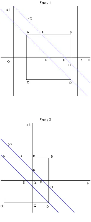
but it will be simpler, or at least more illuminating, to do it graphically. In the plane of coordinates θ and εj, the support of the uniform conditional
distribution of the joint variable (θ, εj)can be represented by a square ABCD
centered on point E of coordinates (k − µ, 0) on the horizontal axis. This is done in Figures 1, 2 and 3. As we have assumed γ ≤ 12, there are only three
possible cases which are represented by these three figures. In Figure 1, the square ABCD is entirely in the area where we have 0 ≤ θ ≤ 1. Figure 2 corresponds to the case where the square ABCD intercepts the vertical axis, in which case we can have θ < 0 or 0 ≤ θ ≤ 1 (but never θ > 1). In figure 3, where the square ABCD intercepts the vertical line where θ = 1, we can have θ > 1 or 0 ≤ θ ≤ 1 (but never θ < 0).
The length of each side of the square ABCD is equal to 2γ. We have AB = CD = AC = BD = 2γ. In these figures we have represented the straight line (Z) of slope (−1) of equation θ + εj = k − µ. We have also
drawn the straight line parallel to (Z) going through point E, which is a diagonal of the square ABCD. This diagonal would be the same as (Z) in the special case µ = µ where there would be no ambiguity.
The straight line (Z) intercepts the horizontal axis at point F, which has coordinates (xi− µ, 0) and is therefore at the right of point E. We have
EF = µ− µ = 2η. Therefore, (Z) intersects the square ABCD in two points G and H if and ony if we have η < γ.
In Figure 1, we always have 0 ≤ θ ≤ 1, which occurs when we have γ ≤ k − µ ≤ 1 − γ. (This case is possible because we have assumed γ ≤ 12). Then, we simply have πµ,µ(k, k) = Prµi=µ,µj=µ(θ + εj > k−µ | xi = k).In the
case η < γ, this probability is given by A(ABCD)A(GBH) ,where A (F) represents the area of figure F. We have A (ABCD) = AB2 = 4γ2and A (GBH) = 12GB2. As we have GB = AB − AG = AB − EF = 2 (γ − η) , we get A (GBH) = 2 (γ− η)2. This gives πµ,µ(k, k) = 12
³
1− ηγ´
2
. In the case η ≥ γ, where the straight line (Z) does not intersects the square ABCD, we have πµ,µ(k, k) =
The case represented in Figure 2 occurs when we have k − µ < γ. In this case, the area where we have θ < 0 should be excluded in order to calculate πµ,µ(k, k). If we have η < γ, then, from Figure 2, this gives πµ,µ(k, k) =
A(GBH)−A(GP R)
4γ2 in the case where (as in Figure 2) G is at the left of P,
i.e. when we have AG < AP. We have AG = EF = 2η, and AP = SO = SE+EO = γ−(k − µ) (because, in Figure 2, point E being on the left of point O, we have k − µ < 0 and therefore EO = − (k − µ)). Thus, the inequality AG < AP gives the condition k − µ < γ − 2η. As we have A (GP R) = 12GP2
and GP = AP − AG = γ − (k − µ) − 2η, this gives πµ,µ(k, k) = 12
³
1− ηγ´2−
1
8γ2 [γ− (k − µ) − 2η]
2
. If G is on the right of P, which occurs when we have k − µ ≥ γ − 2η, then there is no relevant area where we have θ < 0, and, as in the first case, we have πµ,µ(k, k) = 12
³
1− ηγ´2. Finally, as in the first case, when we have η ≥ γ, we always have πµ,µ(k, k) = 0.
In the third case, depicted in Figure 3, the square ABCD intercepts the vertical line θ = 1. This occurs when we have k − µ > 1 − γ. Then all the area where we have θ > 1 should be included. If we have η < γ, this means that, in Figure 3, to the area of the triangle GBH, we have to add the area of LNDH. We therefore have πµ,µ(k, k) = A(GBH)+A(LHND)4γ2 . We can
write A (LHND) = A (LIH) + A (IHND). We have A (LIH) = 12IH 2
and A (IHND) = IH.HD. We have HD = EF = 2η and IH = OT − 1 = OE + ET − 1 = k − µ + γ − 1. Let us define ν ≡ k − µ + γ − 1. we get A (LIH) = 12ν
2
and A (IHND) = 2ην. This implies πµ,µ(k, k) = 1 2 ³ 1−γη´ 2 + 8γ12 (ν
2+ 4ην) . However this calculus is valid only when G is
on the left of M, as in Figure 3. This occurs when we have AG < AM. As we have AG = EF = 2η and AM = AB − IH = 2γ − ν, this inequality can be written 2η < 2γ − ν, or equivalently ν < 2 (γ − η) , which can also be written k− µ < 1 − γ + 2 (γ − η) . When this inequality is not verified, i.e. when we have k − µ ≥ 1 − γ + 2 (γ − η) , then G is on the right of M, and we simply have πµ,µ(k, k) = A(MBND)4γ2 . As we have A (MBND) = IH.BD = 2νγ, this
implies πµ,µ(k, k) = 12νγ. Finally, when we have η ≥ γ, then we also have
πµ,µ(k, k) = A(MBND)4γ2 =
1 2 ν γ.
These results can be summarized in the following Proposition:
Proposition 3 (i) In the case k − µ < γ − 2η, when we have η < γ, we get πµ,µ(k, k) = 1 2 µ 1− η γ ¶2 − 8γ12 [γ− (k − µ) − 2η] 2 (9) and, when we have η ≥ γ, we get πµ,µ(k, k) = 0
(ii) In the case γ − 2η ≤ k − µ ≤ 1 − γ, when we have η < γ, we get πµ,µ(k, k) = 1 2 µ 1− η γ ¶2 (10) and, when we have η ≥ γ, we get πµ,µ(k, k) = 0
(iii) In the case η < γ and 1 − γ < k − µ < 1 − γ + 2 (γ − η) we get πµ,µ(k, k) = 1 2 µ 1− η γ ¶2 + 1 8γ2 ¡ ν2+ 4ην¢ (11)
where we have defined
ν≡ k − µ + γ − 1 (12)
(iv) In the case k − µ ≥ 1 − γ + 2 (γ − η) if we have η < γ, and in the case k − µ > 1 − γ if we have η ≥ γ we get
πµ,µ(k, k) =
1 2 ν
γ (13)
The equilibrium condition is πµ,µ(k, k) = λ.First, consider the case η < γ
. Then, if we look for a solution satisfying the inequality k − µ < γ − 2η of case (i) of Proposition 2. In the case η < d, using (9) , πµ,µ(k, k) = λ gives
a second order equation in the variable (k − µ). It can easily be shown that this equation has solutions if and only if we have 0 < λ < 1
2
³
1− ηγ´2; and, when this last inequality is satisfied, there is a unique solution satisfying the inequality k − µ < γ − 2η, and this is the solution given by (5) and (6) of Proposition 2.
In the same way, we can look for a solution satisfying 1 − γ < k − µ < 1− γ + 2 (γ − η) of case (iii) of Proposition 3. Using (12) , this inequality can be written 0 < ν < 2 (γ − η) . Using (11) , πµ,µ(k, k) = λ gives a second
order equation in ν which is ν2 + 4ην
− 4γ2(2λ
−³1− ηγ´
2
) = 0. It can easily be shown that this equation has a solution satisfying the inequalities 0 < ν < 2 (γ− η) if and only if we have 12³1− ηγ´
2
≤ λ < 1 − γη, and this
solution is then unique and is given by (5) and (7) of Proposition 2.
When we look for a solution satisfying inequality k −µ ≥ 1−γ +2 (γ − η) of case (iv) of Proposition 3, using (13) , we get ν = 2λγ; using (12) , this gives the solution for k given by (5) and (8) of Proposition 2. This solution satisfies the corresponding inequality k − µ ≥ 1 + γ − 2η, if and only if we have λ ≥ 1 − γη.
The case (ii) of Proposition 3, where we look for a solution satisfying γ − 2η ≤ k − µ ≤ 1 − γ is peculiar because πµ,µ(k, k) is always equal to
1 2
³
1−γη´
2
in the case η < γ (and to zero if η ≥ γ). Consequently, if we have λ = 12³1−γη´
2
and η < γ, then the equilibrium condition πµ,µ(k, k) = λcan
be satisfied for any value of k − µ such that we have γ − 2η ≤ k − µ ≤ 1 − γ. Then, any switching point satisfying this inequality gives an equilibrium.
Now consider the case η ≥ γ. Proposition 3 implies that we have πµ,µ(k, k) =
0 if we have k − µ ≤ 1 − γ, and πµ,µ(k, k) = 12νγ if we have k − µ > 1 − γ.
As we have λ > 0, the equilibrium condition πµ,µ(k, k) = λin the case η ≥ γ
requires k − µ > 1 − γ. Then, this solution is given by ν = 2λγ, which yields the solution for k given by case 2, and therefore by equations (5) and (8) , of Proposition 2. Note that for all possible values of λ (which satisfy 0 < λ < 1) this solution verifies the required inequality k − µ > 1 − γ.
Finally, at the beginning of the Appendix, in order to calculate the prob-ability distribution of θ, conditional on having xi = k,we have assumed that
k belongs to the interval£µ− δ2, µ + 1 +δ2¤.We therefore have to verify that the equilibrium values of k we found satisfy this requirement. This can be seen in the following way. In the extreme case k = µ − δ2, we would be in
the case of Figure 2 where E would have coordinates ¡−δ2, 0¢. As we have assumed γ ≤ δ
2, this implies that the square ABCD would be necessarily
entirely contained in the region θ ≤ 0 on the left of the vertical axis. We would thus have πµ,µ(k, k) = 0 in this case. In the same way, in the other
extreme case k = µ + 1 + δ
2, we would be in the case of Figure 3 where E
would have coordinates ¡1 +δ2, 0¢. As we have assumed γ ≤ 2δ, this implies that the square ABCD would be necessarily entirely contained in the region θ ≥ 1 on the right of the vertical axis θ = 1. This would give πµ,µ(k, k) = 1 in
this case. But, in Figures 1, 2 and 3, an increase in k has the effect of shifting the square ABCD and the straight line (Z) to the right by the same amount. Thus, a greater k decreases the probability of having θ < 0 or increases the probability of having θ > 1 (or possibly could leave them unchanged). This implies that πµ,µ(k, k) is a non decreasing function of k (this property could
also easily be seen from Proposition 3). As a consequence, because we have 0 < λ < 1, the solution of the equation πµ,µ(k, k) = λ necessarily belongs to
Figure 1 O A B D C E F G H 1 θ ε j (Z) Figure 2 O A B C D E F H R P G θ ε j Q S (Z)
Figure 3 A B C D E F G H I L M N O θ ε j 1 (Z) T
References
[1] Carlsson, H. and E. van Damme (1993), "Global Games and Equilibrium Selection", Econometrica, Vol. 61, No. 5, 989-1018.
[2] Cheli, B. and P. Della Posta (2007), "Self-fulfilling Currency Attacks with Biased Signals, Journal of Policy Modeling, 29, 381-396. [3] Diamond, D. and P. Dybvig (1983), Bank Runs, Deposit Insurance, and
Liquidity", Journal of Political Economy, 91, 401-419.
[4] Ellsberg, D. (1961),"Risk, Ambiguity, and the Savage Axioms", Quar-terly Journal of Economics, 75,.643-669.
[5] Gajdos, T, Tallon, J.M. and J.-C. Vergnaud (2004), "Decision Making with Imprecise Probabilistic Information", Journal of Mathematical Economics, 40, 647-681.
[6] Gilboa, I. and D. Schmeidler ((1989), "Maximin Expected Utility with Non-Unique Prior", Journal Mathematical Economics,18, 141-153. [7] Kawagoe, T. and T. Ui (2010), "Global Games and Ambiguous
[8] Knight, F.H. (1921), Risk, Uncertainty and Profit, Boston: Houghton Mifflin.
[9] Metz, C.E. (2003), "Private and Public Information in Self-Fulfilling Currency Crises", June.
[10] Morris, S. and H.Y. Shin (1998), "Unique Equilibrium in a Model of sel-fulfilling currency attacks, American Economic Review, 88 (3), 587-597.
[11] Morris, S. and H.Y. Shin (2003), "Global Games: Theory and Applica-tions", in Advances in Economics and Econometrics: (Proceedings of the Eighth World Congress of the Econometric Society),ed. by M. Dewatripont, L.P. Hansen and S.J. Turnovsky, Cambridge University Press.
[12] Morris, S. and H.Y. Shin (2004), "Cordination and the Price od Debt", European Economic Review, 48, 133-153.
[13] Mukerji, S. and J.-M. Tallon (2004), "An overview of economic appli-cations of David Schmeidlers’s models of decision making under un-certainty" in I.Gilboa, (ed), Uncertainty in Economic Theory: A collection of essays in honor of David Schmeidler’s 65th birthday, Routledge Publishers.
[14] Obstfeld, M. (1996), "Models of Currency Crisiswith Self-Fulfilling Fea-tures", European Economic Review, 40, 1037-1047.
[15] Schmeidler, D. (1989), "Subjective Probability and Expected Utility without Additivity", Econometrica, Vol.57, No. 3, May, 571-587. [16] Ui, T. (2009), "Ambiguity and Risk in Global Games", June.