HAL Id: hal-02153840
https://hal.archives-ouvertes.fr/hal-02153840
Preprint submitted on 12 Jun 2019
HAL is a multi-disciplinary open access archive for the deposit and dissemination of sci-entific research documents, whether they are pub-lished or not. The documents may come from teaching and research institutions in France or abroad, or from public or private research centers.
L’archive ouverte pluridisciplinaire HAL, est destinée au dépôt et à la diffusion de documents scientifiques de niveau recherche, publiés ou non, émanant des établissements d’enseignement et de recherche français ou étrangers, des laboratoires publics ou privés.
Endogenous fluctuations and the balanced-budget rule:
taxes versus spending-based adjustment
Maxime Menuet, Alexandru Minea, Patrick Villieu
To cite this version:
Maxime Menuet, Alexandru Minea, Patrick Villieu. Endogenous fluctuations and the balanced-budget rule: taxes versus spending-based adjustment. 2019. �hal-02153840�
Endogenous fluctuations and the balanced-budget rule:
taxes versus spending-based adjustment
Maxime Menueta,1, Alexandru Mineaa,b, Patrick Villieuc
aSchool of Economics & CERDI, Universit´e d’Auvergne bDepartment of Economics, Carleton University, Ottawa, Canada cUniv. Orl´eans, CNRS, LEO, UMR 7322, FA45067, Orl´eans, France
Abstract
The present paper develops a simple theoretical setup to examine the role of the tax-spending mix of fiscal adjustments on aggregate (in)stability in indebted economies. To this end, we build an AK endogenous growth model with public debt dynamics. If the adjustment of the government’s budget constraint is based on a single instrument (taxes or public spending), the economy converges towards a high-growth path. With mixed adjustment, however, another equilibrium appears (the no-growth path) that can be locally over-determine (unstable) or under-determined (stable). A hopf bifurcation can occurs at the border between the last two cases, which leads to cyclical dynamics. We also show that global indeterminacy is likely to emerge if fiscal adjustment is mainly based on public spending. A calibration of the model shows that area of indeterminacy covers reasonable values for parameters.
Keywords: Endogenous growth; indeterminacy; balanced-budget rules; hopf bifurcation
1. Introduction
In response to the Great Recession and to the long-lasting increase of public debt since four decades, many OECD countries implemented fiscal consolidation programmes. However, empirical researches on the macroeconomic effects of these programmes remain unsettled. Some authors find expansionary austerity episodes (Giavazzi and Pagano,
1990;Briotti,2005), while others join traditional textbook Keynesian models highlighting the adverse effects of fiscal austerity on economic growth (Perotti, 2011).
Beyond these conflicting views, the current consensus emerging from recent empirical research is that the composition of fiscal consolidations (tax increases vs spending cuts) matters. Typically, robust evidences suggest that consolidations based on tax-increases generate larger fluctuations and output losses compared to consolidations relying on re-ductions in government spending, including both public investment and government con-sumption or transfers.2 From a theoretical perspective, such findings can be related to
1Corresponding author: [email protected].
2This result is established using VAR (Perotti and Alesina,1995;Alesina and Ardagna,2010), or with
the narrative IMF data ofPescatori et al. (2011), asAlesina and Ardagna (2013);Alesina et al.(2017, 2018). This result contrast with standard Keynesian works predicting that spending cuts are always recessionary and that multiplier for spending are higher than for taxes (Gal´ı et al., 2007; DeLong and Summers,2012).
the aggregate fluctuation in the form of belief-driven fluctuations in neoclassical growth models. Indeed, in these models, a tax-based (TB) fiscal adjustment can produce ag-gregate instability (Schmitt-Groh´e and Uribe,1997), while there is a stable staddle-path to the steady state under a expenditure-based (EB) adjustment (provided that public spending is useless, Guo and Harrison, 2004). However, this theoretical literature has two shortcomings. First, it rests on the assumption of a balanced-budget rule (BBR), without accounting for public debt. Yet, public deficits and debts characterize most de-veloped countries since the mid-1970, and the implemented consolidation plans mostly aim at reaching a sustainable public debt path.3 Second, these models only consider a
single instrument-based adjustment (taxes or spending), contrasting with effective fiscal adjustment plans, which are often complex policy packages that closely associate the tax and spending sides.4
The goal of this paper is to provide a simple theoretical setup to examine the role of the tax-spending mix of fiscal adjustments on aggregate (in)stability in indebted economies. To this end, we build a continuous-time one-sector endogenous growth model with two innovative features that reflects stylized facts of fiscal adjustments.
On the one hand, we consider a generalized BBR, which allows taking account of public debt. Indeed, the economies that adopt a BBR generally have a positive debt at the time they implement the rule (and, as Lled´o et al., 2017, shows, the implementation of the BBR mostly results from the presence of a high public debt).5 This generalized
BBR can generate a complex dynamics of the debt-to-output ratio, even if the public debt level is constant over time.
On the other hand, we specify a general adjustment scheme, such that the debt-burden is covered both by cuts in public spending and rises in taxes, and we carefully examine the effect of the sharing of fiscal adjustment between the two instruments. In-deed, historical evidences show that both expenditure and revenue items contribute to fiscal adjustment. For example, Alesina and Ardagna find contributions around 35% for EB and 65% for TB adjustment in OECD contractionary episodes (1970-2007). Based
3The deficit-to-GDP ratio was around 2.5% on average in OECD countries in the period 1970-2005,
and this ratio increased since the Great Recession (according to the 2017 IMFs World Economic Outlook, average general government gross debt in ratio of GDP in developed countries rose from around 72% in 2007 to roughly 105% in 2007).
4For example,Alesina et al. (2015) identify TB (resp. EB) fiscal adjustments, as episodes such that
(announced or unexpected) changes in taxes (resp. expenditures) are larger than changes in expenditures (resp. taxes). They conclude that fiscal adjustments mostly mix changes in taxes and expenditures: in the 60 plans documented, around 40% consist in years of TB and 60% in years of EB adjustments.
5A number of recent works have shown that endogenous growth setups are a useful framework for
analyzing the effects of a continuous grow of public debt in the long run; see, e.g., Minea and Villieu (2012); Nishimura et al. (2015a); Boucekkine et al. (2015); Nishimura et al. (2015b); Menuet et al. (2018a). Albeit we focus here on BBR regimes, our model can be extended to deficit rules without qualitative changes (see, in particular,Minea and Villieu, 2012; Menuet et al.,2018a).
on a simple small-scale (two dimensional) dynamic system, we notably show that small changes in the tax-spending mix generate radical shifts in the dynamic properties of the economy, i.e., bifurcations.
Our results are as follows.
(i) If the fiscal adjustment is based on a single instrument, there is a unique well-determined positive balanced-growth path (BGP) in the long run. With EB adjustment, the steady state is unique, while under TB adjustment, the interaction between the government’s budget constraint and households optimal saving behavior gives birth to a pair of BGPs: a high-growth path with zero debt and a no-growth trap with high debt. However,the latter is unstable and can be removed thanks to local dynamic analysis.
(ii) With mixed adjustement of taxes and public spending, multiplicity cannot be excluded. Indeed, in this case, while the high equilibrium is always saddle-path stable, the topological behavior of the no-growth trap is more complex. Depending on the relative weigh of TB adjustment (that we use as a bifurcation parameter), the no-growth trap can be locally over-determined (unstable), or under-determined (stable). Effectively a subcritical Hopf bifurcation can occur, leading to cyclical dynamics.
(iii) The simplicity of our framework allows fully characterizing the global dynamics of the economy. We notably show that global indeterminacy is likely to emerge if fiscal adjustment is mainly based on public spending. A calibration of the model show that area of indeterminacy covers reasonable values for parameters, since the share of TB ad-justement that gives rise to the Hopf bifurcation is around 40%, close to Alesina et al. and Dvies empirical findings.
Although stylized, our model addresses major long-lasting topics in macroeconomics. First, our paper complements the fast-growing literature on indeterminacy in en-dogenous growth models.6 Starting from the seminal paper of Matsuyama (1991), local
and global indeterminacy come from public capital externality (productive or welfare-enhancing public spending), increasing returns, or interactions in two-sector frameworks7.
In contrast, in our model, global indeterminacy is established in a simple one-sector model with wasteful public spending, and does not fundamentally rest on increasing return in production. Indeed, under a BBR, the non-trivial dynamics of the debt-to-capital ratio give rise to complex interactions between the government’s budget constraint and the households’ saving behavior.8
6See the surveys of Benhabib and Farmer (1999), chap. 6, or Mino et al. (2008) regarding the local
indeterminacy.
7See, e.g., Benhabib et al. (1994); Benhabib and Nishimura (1998); Matsuyama (1999); Benhabib
et al.(2000);Brito and Venditti(2010);Mattana et al.(2012);Nishimura et al. (2013), among others.
8Some papers have shown that endogenous growth models with public debt generate indeterminacy
Second, in our model, two instruments (taxes and pubic spending) can adjust jointly the government’s budget constraint. This is an important feature because, to the best of our knowlged, this is the first paper that provides a theoretical basis to the large empirical literature emphasizing that fiscal adjustments closely associate both tax and spending sides.9
The remainder of the paper is organized as follows. Section 2 presents the model, section 3 studies local dynamics, section 4 provides a numerical example, section 5 ex-plores the global dynamics, section 6 discusses findings in term of economic policy and concludes.
2. The model
We consider a simple continuous-time endogenous-growth model with a representative individual, who consists of a household and a competitive firm, and a government. All agents are infinitely-lived and have perfect foresight.
2.1. Households
The representative household starts at the initial period with a positive stock of capital (K0) and a given dotation of time that is inelastically devoted to labor (thus, labor supply L is exogenous). He chooses the path of consumption {Ct}t≥0, and capital {Kt}t>0, so as to maximize the present discount value of its lifetime utility.
U = ∞ !
0
e−ρtu(Ct)dt, (1)
where ρ∈ (0, 1) is the subjective discount rate
As usual, we define a constant-elasticity of substitution (CES) utility function
u (Ct) = " S S−1 # (Ct)S−1S − 1 $ , if S ̸= 1, log (Ct) , if S = 1, (2) with S :=−u′′(C
t)Ct/u′(Ct) > 0 the elasticity of intertemporal substitution in consump-tion.
Households use their income (Yt = rtKt+ wtLt) to consume (Ct), invest ( ˙Kt), buy government bonds (Bt), with a real expected return ˜Rt, and pay taxes (τtYt, where τt is a proportional income tax rate); hence the following budget constraint
˙
Kt+ ˙Bt= ˜RtBt+ (1− τt)(rtKt+ wtL)− Ct+ Xt. (3)
9In previous theoretical literature, the fiscal adjustment is based on a single instrument: the
distor-tionary taxation with a fixed exogenous spending (Schmitt-Groh´e and Uribe,1997;Giannitsarou,2007), or the public spending with a fixed tax rate (Guo and Harrison,2004,2008).
Xt is a transfer from the government, to be defined below.
When studying the dynamics of public debt, it is important to distinguish between the return of capital rt and the the return of public debt, say Rt. Effectively, history has shown that substantial risk premia on public debt can appear at high public-debt ratios. To introduce this element in our setup without complexify the model with an explicit treatment of financial imperfections, we imagine the following story. We suppose that, at the instant they make portfolio choices (i.e., at the beginning of the period), households expect that a fraction χt ∈ (0, 1) of public debt may not be repaid. Thus, in the budget constraint (6), the return of public debt must be weighed by the probability of a future “haircut” (1 − χt). If the real return of public debt is Rt, the expected return for households is only ˜Rt:= Rt(1− χt). However, in equilibrium, the government will always honor his commitments, so that the totality of public debt will be repaid. To describes this fact, we consider that households receive, at equilibrium (i.e., at the end of the period), a lump-sum transfer Xt that corresponds to the remaining part of interest payments.10 Therefore, even if the government does not default in equilibrium,
households do not exclude the possibility of default at the time they make their portfolio choice.
Such a framework generates a risk premium on public debt, without considering ex-plicit microfoundations of risk. Effectively, the trade-off between public bonds and private capital provides the following condition: (1 − χt)Rt = (1− τt)rt, with 1/(1− χt) ≥ 1 being the risk premium. In order to endogenize this premium, we consider that χt is an increasing function of the ratio of aggregate public debt to GDP, namely: χt = χ( ¯Bt/ ¯Yt), with χ′(·) ≥ 0, where ¯Bt and ¯Yt represent global equilibrium variables that the household takes as given in its program (aggregate externality). Then, by defining θ( ¯Bt/ ¯Yt) := 1/(1− χ( ¯Bt/ ¯Yt)), we have
Rt = θ( ¯Bt/ ¯Yt)(1− τt)rt.
The term θ( ¯Bt/ ¯Yt)≥ 1 represents the risk premium on public debt, which positively depends on the public debt ratio.
The first order condition for the maximization of the household’s programme gives rise to the Keynes-Ramsey relationship
˙ Ct
Ct = S ((1− τt)rt− ρ) . (4)
10Hence, at equilibrium, each household receives a lump-sum transfer X
t = χtRtB¯t/N , where ¯Bt
represents total public debt issued by the government and N the number of households in the economy (that we have normalized to N = 1).
In addition, the optimal path has to verify the set of transversality conditions lim t→+∞{exp(−ρt) u ′(Ct) Kt} = 0 and lim t→+∞{exp(−ρt) u ′(Ct) Bt} = 0, ensuring that lifetime utility U is bounded.11
2.2. Firms
Output (Yt) is produced using a constant returns-to-scale technology with a capital externality, namely
Yt = AKtα(LtKt)¯ 1−α,
where A > ρ/α is a scale parameter (that ensures positive growth solutions) and α∈ (0, 1) is the elasticity of output to private capital. Kt stands for private capital and ¯Kt is the economy-wide level of capital that generates positive technological spillovers onto firm’s productivity (Romer, 1986).
The first order conditions for profit maximization (relative to private factors) are
rt= αYt
Kt, (5)
wt= (1− α) Yt
Lt. (6)
with, at equilibrium, Lt = L. We henceforth normalize L = 1. 2.3. The government
The government provides public expenditures Gt, levies taxes Tt, and borrows from households. Fiscal deficit is financed by issuing debt ( ˙Bt); hence, the following budget constraint
˙
Bt= ˜RtBt+ Gt− Tt− Xt= RtBt+ Gt− Tt, (7) Without loss of generality, we define tax and public spending ratios as τt = Tt/Yt, and gt = Gt/Yt, respectively. At this stage, the government has three instruments: the tax rate (τt), the public spending ratio (gt), and the public debt path ( ˙Bt).
The paper aims to study the implications of the BBR. Without public debt, such a rule corresponds to Gt = Tt. However, the economies that adopt a BBR do not necessarily have zero debt at the time of adoption. On the contrary, almost all countries having adopted a BBR were (sometimes highly) indebted countries. For an economy starting with an initial public debt B0, the BBR (i.e. ˙Bt= 0⇔ Bt= B0,∀t) thus corresponds to RtB0+ Gt= Tt ⇒ RtB0+ gtYt = τtYt. (8)
11On the BGP associated to constant growth and interest rates (γ∗and r∗, respectively), the
transver-sality conditions correspond to the no-Ponzi game constraint γ∗< r∗. Such condition ensures that public
debt will be repaid in the long run, and does not precludes the possibility that γ > r in the short run.
The presence of a positive public debt level (B0) has crucial implications, since our model can exhibit complex dynamics of the public debt ratio (B0/Yt), even in the presence of the BBR.
2.4. Equilibrium
At equilibrium, we have Kt= ¯Kt, which in turn leads to the simple social technology
Yt= AKt. (9)
Thanks to constant-returns at the social level, endogenous growth can emerge, despite decreasing returns of private capital from the individual firm’s perspective. Therefore, using (5), the real interest rate becomes, at equilibrium
rt = αA. (10)
To obtain long-run stationary ratios, we deflate consumption and public debt by output and we use minuscule letters to depict ratios, namely: ct := Ct/Ytand bt = B0/Yt. Thus, the return of government bonds: Rt = θ(bt)(1− τt)rt.
The path of the capital stock is given by the goods market equilibrium ˙ Kt Kt = A(1− gt− ct). (11) From (7), we obtain ˙bt bt = ˙ Bt Bt − ˙ Kt Kt = Rtbt+ gtyt− τtyt− ˙ Kt Kt, hence, under the BBR (8),
˙bt=−btK˙
K. (12)
From (4), (10), (11), and (12), the reduced-form of the model is ⎧ ⎪ ⎪ ⎨ ⎪ ⎪ ⎩ ˙ct
ct = S[α(1− τt)A− ρ] − A(1 − gt− ct) (a), ˙bt =−Abt(1− gt− ct) (b).
(13)
Considering the BBR, the government must select the set of policy instrument {τt, gt}t≥0 to balance its budget each period. Thus, we must specify an adjustment scheme for gov-ernment’s finance. Deflating (8) by Yt and using (10), we have
where x(bt) := αAθ(bt)bt is the (gross) debt burden, with x′(bt)≥ 0.
Therefore, any increase of the public debt ratio (bt) requires a lower public spending ratio (gt) and/or a higher the tax rate (τt). Let us introduce a general adjustment scheme, such that the debt burden is shared between the two instruments, namely
τt = τ (bt), and gt= g(bt),
where g, τ : R+ (→ [0, 1] are C2-functions, with g(0) = τ (0) =: τ
0 ∈ (0, ¯τ), where ¯τ := 1− ρ/αA ∈ (0, 1), and −R′(bt)bt− R(bt)≤ g′(bt)≤ 0. The latter assumption means that debt-burden-increases are partially covered by cuts in public spending.12 This ensures
that τ′(bt) ≥ 0, namely that the residual part of the debt burden is covered by tax-increases.13
2.5. Steady states
We define a BGP as a path on which consumption, capital, and output grow at the same (endogenous) rate, namely (we henceforth omit time indexes)
γ∗ := ˙C/C = ˙K/K = ˙Y /Y.
Proposition 1. There is a non-empty set of parameters, such that
i. There are two candidate long-run solutions: a high steady state (H), characterized by positive growth (γH > 0) and zero debt (bH = 0), and a low steady state (L), characterized by zero growth (γL = 0) and positive debt (bL> 0).
ii. If τ′ = 0, only the high steady-state solution emerges, iii. If τ′ > 0, the two solutions are feasible (multiplicity).
Proof.
(i) By setting ˙b = 0 in (13b), we have either b > 0 ⇒ γ = 0 – this defines the low BGP (L) –, or γ > 0⇒ b = 0 – this defines the high BGP (H).
(ii) If τ′ = 0, i.e. τ (bt) = τ0, for any bt ≥ 0, the rate of economic growth is: γH = S[αA(1 − τ0) − ρ]. As τ0 < ¯τ , we have γH > 0; hence bH = 0. Therefore, cH = 1− g(0) − γH/A. This solution is well defined if cH > 0. As g(0) = τ (0) = τ0, this requires that S < ¯S, with ¯S := (1− τ0)/[(1− τ0)− ρ/A] > 1; which is true for usual values of the elasticity of intertemporal substitution in consumption ( S ≤ 1).
(iii) If τ′ > 0, there are two kinds of solutions. First, according to point (i) we find the same solution as in point (ii), namely: γH = S[αA(1− τ(0)) − ρ] = S[αA(1 − τ0)− ρ]. Second, we have a zero-growth solution at γL= 0⇔ cL= 1−g(bL), where, by introducing in (13a): bL= τ−1(1− ρ/αA). This solution is well defined if ρ < αA, and g(bL) < 1.
12Indeed: d
dbt{Rtbt+ gt} ≥ 0 ⇔ −R
′(b
t)bt− R(bt) ≤ g′(bt). 13Effectively, under the BBR, τ
t= gt+R(bt)bt; hence τ′(bt) = R′(bt)bt+R(bt)+g′(bt) ≥ 0. Noteworthy,
since θ(0) < +∞, the government’s budget constraint imposes that τ(0) = g(0) when bt= 0.
! The multiplicity comes from the interaction between the government’s budget con-straint and household’s saving behaviour. Especially, if public spending is the only adjust-ment variable in governadjust-ment’s budget constraint (τ′ = 0), there is one unique steady-state solution (the high BGP).14Indeed, in this case, the long-run rate of economic growth (as
defined in the Keynes-Ramsey relationship) is positive and independent of public debt, such that the no-growth solution cannot happen.
With a time-varying tax-rate (τ′ > 0), however, the net return of capital depends on public debt in the Keynes-Ramsey rule. In steady state, the BBR is then consistent with two situations. In the first case, public debt is zero in the long-run, which implies a zero debt burden. As a result, the tax-rate is low, thus leading to the high BGP. In the second case, in contrast, expected long-run public debt is high and generates a high risk premium that forces the government to set a high tax-rate. Then, in steady state, the long-run public debt ratio is such that its burden completely stifles economic growth, given the tax-rate that must be imposed. In this case, the economy is trapped into a no-growth BGP.
3. Local Dynamics
By linearization, in the neighborhood of steady-state i, i ∈ S = {L, H}, the system (13) behaves according to ( ˙ct, ˙bt) = Ji(ct− ci, bt− bi), where Ji is the Jacobian matrix. The reduced-form includes one jump variable (the consumption ratio c0) and one pre-determined variable (the public-debt ratio b0, since initial stocks of public debt B0 and private capital K0 are predetermined). Thus, for BGP i to be well determined, Ji must contain two opposite-sign eigenvalues. Using (13), we compute
Ji = ) CCi CBi BCi BBi * , where CCi = Aci, (15) CBi = Aci[g′(bi)− αSτ′(bi)], (16) BBi =−γi+ Abig′(bi), (17) BCi = Abi. (18)
14However, the multiplicity would appear again with productive public spendingMenuet et al.(2018a),
Hence, the trace and the determinant of the Jacobian matrix are, respectively
Tr(Ji) = Aci− γi+ Abig′(bi), (19) det(Ji) = −Aγici+ αA2Scibiτ′(bi). (20) The following theorem establishes the topological behaviour of each steady-state.
Theorem 1. (Local Stability)
• The high BGP is locally determined (saddle-point stable). • The topological behaviour of the low BGP is the following.
∗ If cL >−bLg′(bL), L is locally over-determined (unstable), ∗ If cL =−bLg′(bL), a Hopf bifurcation occurs,
∗ If cL <−bLg′(bL), L is locally under-determined (stable). Proof.
(i) det(JH) = −AγHcH < 0, namely there are two opposite-sign eigenvalues. Conse-quently, H is saddle-point stable.
(ii) det(JL) = αA2ScLbLτ′(bL) > 0, and Tr(JL) = A(cL+ bLg′(bL)). Therefore, if cL< (>)− bLg′(bL), there are two eigenvalues with negative (positive) real part, so that L is stable (instable). At cL = −bLg′(bL), the Hopf bifurcation arises, and a periodic orbit through a local change in the stability properties of L appears. As cL= 1− g(bL), the Hopf bifurcation occurs at a point bL
h such that 1− g(bLh) = −bLhg′(bLh). By defining the elasticity e(b) := −bg′(b)/g(b), the Hopf bifurcation arises at g(bL
h) = 1/(1 + e(bLh)). This, in turn, defines a critical value for some parameter included in bL
h (given existence and uniqueness restrictions, see our numerical results in section 4).
! The different stability properties of the two equilibria comes from the dynamics of the public debt. In the neighborhood of the high steady state, economic growth is high enough to overcome the unstable dynamic of the public debt-to-output ratio. Hence, the topological behaviour of the high BGP does not depend on the adjustment scheme of public finance. Effectively, this steady state is saddle-path stable, independently on the specification of functions g(·) and τ(·).
In contrast, the local determinacy of the low BGP crucially depends on the form of the adjustment scheme of public finance, through functions g(·) and τ(·). Especially, a necessary condition for the Hopf bifurcation to occur is that public expenditures (taxes) negatively (positively) react to public debt, as establishes the following lemma.
Lemma 1. If (i) τ′ = 0 or (ii) g′ = 0, the model is well determined.
Proof. (i) If τ′ = 0 (i.e. τ
t =: τ0,∀t), there is a unique positive BGP, namely γH = S[α(1− τ0)A− ρ]. This BGP is locally well determined, because, from (20), det(J) = −AγHcH < 0.
(ii) If g′ = 0 (and τ′ > 0), then cL > −bLg′(bL) = 0, the low BGP is unstable and
indeterminacy is removed. !
Contrary to the high BGP, around the no-growth solution (if this solution exists, i.e. τ′ > 0), the snowball effect of the debt burden cannot be avoided, giving rise to the emergence of a cyclical dynamics. If public spending does not react to the debt burden or lowly reacts, this dynamics is explosive, while in the opposite case, the no-growth solution becomes locally stable and can be reached, but at the price of (possibly large) oscillations during the transition path. This finding stresses the importance of having both an adjustment of public spending and resources in the dynamics of the model.
4. A numerical exploration
To assess the dynamics of the low BGP, it is necessary to characterize the nature of the Hopf bifurcation. Effectively, depending on the value of the first Lyapunov coefficient, the bifurcation can be subcritical or supercritical. To compute this coefficient, we must characterize explicitly the adjustment scheme of government’s finance, i.e. define explicit functions τ (·) and g(·). From Eq.(14), public spending and taxes must adjust to changes in the public debt burden, as we have seen. We consider here that a share η ∈ (0, 1) of debt-burden increases are covered by tax-increases, and a share 1− η by a cuts in public spending, namely
τt= ηRtbt+ τ0, and gt= τ0− (1 − η)Rtbt,
where τ0 ≥ 0 is a constant (that corresponds to the long-run tax rate in the high BGP) that ensures gt ≥ 0. Obviously, if η = 0 (resp. η = 1), taxes (resp. public spending) is the only adjustment variable to the debt burden. Then, the equilibrium can be fully char-acterized by considering a specific function for the (gross) debt burden. In the following, we consider a iso-elastic function: x(bt) := αAbε
t, with ε > 1.
In this case, the value of η that gives rise to the Hopf bifurcation is (see Appendix B)
ηh = (α0− 1)(ε − α0)
α0+ (α0− 1)(ε − α0), (21) where α0 := αA(1− τ0)/ρ > 1.15 We can remark that ηh ∈ (0, 1) under the sufficient condition that ε > α0.16
15α
0> 1 is a necessary condition for the public debt to be positive. 16η
h is positively related to the elasticity of the debt burden function, with ηh = 0 if ε = α0 and
Our numerical results are based on reasonable values of parameters. Regarding house-hold’s preferences, we choose ρ = 0.05,17 and a logarithmic utility function (S = 1).
Re-garding the technology, we set A = 0.3 to obtain realistic rates of economic growth and real interest rate, and the capital share in the production function is α = 0.3. Regarding the government’s behavior, the long-run value of the tax-rate is fixed at τ0 = 0.4 in the high BGP, corresponding to long-run average values in the US or OECD from 1950 to 2015, and the elasticity of the debt burden is chosen to be ε = 10. The benchmark value of η is 0.5, but this parameter will be scanned over a large range of values to verify the presence (or not) of a Hopf bifurcation. For these parameters’ values, the corresponding growth rate is γH ≃ 0.4% in the high BGP (with γL = 0 in the low BGP), and the associated public debt ratios are bH = 0 and bL≃ 1.06.
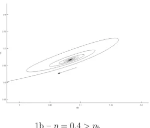
The Hopf bifurcation occurs at ηh ≃ 0.38 corresponding to a public debt ratio of bL ≃ 1.09. For values of the elasticity less than ηh, the low BGP is stable, as in Figure 1a, while it is unstable for values above ηh (Figure 1b). With ηh = 0.38, the corresponding value for the risk premium is around 5%, which seems reasonable for high indebted countries.
1a – η = 0.35 < ηh 1b – η = 0.4 > ηh
Figure 1 – The subcritical Hopf bifurcation
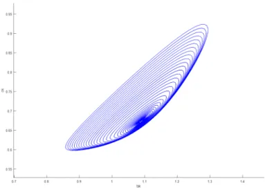
Simulations using c⃝ matcont show that the first Lyapunov coefficient is positive (approximatively 1.00), thus defining a subcritical Hopf bifurcation. At η = ηh the low BGP is neither stable or unstable, but for slightly lower values of η, closed orbits arise that enclose the low BGP. These orbits becomes larger the lower the value of η (see Figure 2). However, these orbits are instable and do not define limit-cycles. Hence, inside the closed orbit, all paths converge towards the low BGP. Consequently, the area of stability
17Since we ignore depreciation, this term can reflect the sum of the risk free (real) interest rate plus
depreciation.
of the low BGP becomes larger as η decreases.18
Figure 2: The family of closed orbits as η declines
Thanks to local analysis, we can now turn to global dynamics.
5. Global Dynamics
The simplicity of our two-dimensional model allows fully characterizing the global dynamics of the system. We can distinguish two cases, depending on the topological behaviour of the low BGP.
In the first configuration, that arises if η > ηh, the low BGP is unstable and only the high BGP can be reached. Figure 4a depicts the phase portrait in this case. There is a heteroclinic connexion between the low and the high BGPs, and the system is both locally and globally well-determined (local and global determinacy).
18The expansion of the closed orbits is limited by the non-negativity condition on public spending.
For some value η = ¯η, we have g=0, hence defining the maximum feasible η and the maximal amplitude in the family of closed orbits.
Figure 4a: Global Dynamics (η > ηh)
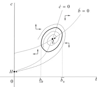
At η = ηh, the Hopf bifurcation arises, and the low BGP is neither unstable or stable. Beyond the Hopf bifurcation, the low BGP becomes stable and there is a closed orbit that encloses it. This gives rise to the second configuration, as depicted in Figure 4b. In this case, η < ηh, and the high BGP is still staddle-path stable and can therefore be reached by a unique well-determined manifold, but the low BGP now is stable, and thus characterized by local indeterminacy. Effectively, inside the closed orbit, all paths converge towards the low BGP, so that the initial consumption ratio and transitory dynamics are undetermined. In addition, if the initial public debt ratio b0 ∈ (b0, ¯b0), where b0 and ¯b0 are, respectively, the leftmost and the rightmost points of the closed orbit, there is global indeterminacy, because either the low or the high BGPs can be reached in the long-run, following an adequate initial jump of the consumption ratio. In this configuration (local and global indeterminacy), both the transition path and the long run equilibrium are subject to “animal spirits”.
Figure 4b: Global Dynamics (η < ηh)
Indeed, the coexistence of multiple feasible equilibrium paths illustrates the possibility of self-fulfilling prophecies: if households think that the economy will end up on the high BGP, then it will; whereas if the low BGP is expected, then this equilibrium will be attained. In such a case, the transition path and the long-run solution of the model are subject to optimistic or pessimistic views on the future. Do the agents expect strong economic growth, the economy will reach the high BGP; do they anticipate a low-growth trap, the economy will be condemned to the low BGP.
Interestingly, as η decreases, the area of indetermination widens, since the values b0 and ¯b0 deviate from each other. Indeterminacy thus can arise for realistic values of the public debt ratio, since, as we have shown in the example of Figure 2, for reasonable pa-rameter values, the largest closed orbit (consistent with a positive public spending ratio) in our benchmark calibration is obtained for b0 ≃ 85% and ¯b0 ≃ 135%.
The intuition of such an indeterminacy is the following. For a given initial public debt ratio (b0), if zero public debt is expected in the future, the after-tax return of private investment is expected to be high, and, at the initial time, households increase their savings, such that the initial consumption ratio c0 is low. This means that, in equilibrium, initial private investment and economic growth will be high, and that the debt ratio will effectively decline in the future, generating a (self-fulfilling) high growth path in the steady-state. On the contrary, if households expect a high debt ratio in the future, the risk premium on public debt will be high, so as the tax rate to finance the debt burden, and the after-tax return of capital will be low. Thus, households initially choose a high initial consumption ratio c0 because the (perfectly expected) return on their savings is expected to be low. In equilibrium, such a consumption ratio crowds out private investment and the initial economic growth is low, which does not allows to
reduce the public debt ratio in the long-run, thus confirming household’s expectations. Therefore, the economy goes towards the no-growth trap.
As we have shown in Lemma 1, indeterminacy crucially depends on the fact that the tax-rate adjusts to the debt burden. This generates the multiplicity of equilibrium paths, because the long-run achievable rate of economic growth depends on the after-tax return of capital.19 But the elasticity of public spending to the debt burden is also a
crucial feature, because it allows stabilizing the low BGP. Effectively, if public spending was independent of the public debt ratio, the low BGP would be unstable, regardless the value of other parameters, and indeterminacy could be removed.
6. Discussion and concluding remarks
This paper shows that local and global indeterminacy can appear when wasteful pubic spending and taxes adjust jointly the government’s budget constraint. Fundamentally, such findings come from the nature of the BBR, which is consistent with non trivial dynamics of the debt ratio when considering endogenous growth. In term of economic policy, our results are mixed.
On the one hand, from the point of view of the high BGP, there is no difference between the two adjustment schemes, because public debt is zero. Furthermore, this BGP is locally well determined, irrespective to the composition of fiscal adjustment. However (partial of full) TB adjustment generates multiplicity of BGPs, with the emergence of a no-growth trap. Such multiplicity can be avoided if public spending fully responds to the debt burden (η = 0). In this case, the tax rate is constant at τ0 and the after-tax expected return of capital is constant, thus removing sunspot equilibria: the no-growth solution vanishes, and the unique long-run BGP is such that public debt is zero, as described in Lemma 1.
This situation pleads for the implementation of full EB adjustments, without any move of the tax rate. Nevertheless, fiscal adjustments exclusively based on expenditure can imply very large cuts in the initial public spending ratio (g0 = τ0−(1−τ0)αAbε
0), especially if the initial public debt is high. Such cuts in public spending could be very costly for households (if, e.g. public expenditures exert a positive externality on households’ welfare), or could simply not be feasible, because public spending cannot take negative values. For countries that are initially highly indebted (in our model, if the initial public debt ratio is larger than ¯b0 := (αA(1− τ0)/τ0)−1/ε), a complete fiscal adjustment with spending-cuts would not be implementable, i.e. an adjustment of the tax ratio to the public debt burden is needed.
On the other hand, if the tax rate partially adjusts to the debt burden ( η > 0), results change dramatically. As we have seen, TB adjustments give birth to a no-growth
19In the context of exogenous growth,Schmitt-Groh´e and Uribe (1997) andGuo and Harrison(2004)
find similarly that the adjustment of the tax-rate is a condition for aggregate instability to emerge.
solution and to multiplicity. From the determinacy perspective, a large adjustement of taxes is then required (η > ηh). Effectively, the lower the share of TB adjustment (η), the larger the area of local stability of the no-growth trap and the more probable the emergence of global indeterminacy. The latter can be removed only if the composition of the adjustment sufficiently relies on taxes (i.e. η > ηh). But strong response of taxes to the debt burden is likely to affect the net return of investment and lower economic growth during the transition path.20 Aggregate instability can therefore be viewed as the
price to be paid for obtaining higher transitional growth.
References
Alesina, A., Ardagna, S., 2010. Large changes in fiscal policy: Taxes versus spending, in: Brown, J.R. (Ed.), Tax Policy and the Economy. The University of Chicago Press, Chicago. volume 24, pp. 35–68. Alesina, A., Ardagna, S., 2013. The design of fiscal adjustments. Tax policy and the economy 27, 19–68. Alesina, A., Barbiero, O., Favero, C., Giavazzi, F., Paradisi, M., 2017. The effects of fiscal consolidations:
Theory and evidence. NBER Working Paper No. 23385 .
Alesina, A., Favero, C., Giavazzi, F., 2015. The output effect of fiscal consolidation plans. Journal of International Economics 96, S19–S42.
Alesina, A., Favero, C., Giavazzi, F., 2018. What do we know about the effects of austerity? NBER Working Paper No. 24246 .
Benhabib, J., Farmer, R., 1999. Indeterminacy and sunspots in macroeconomics, in: Taylor, J., Wood-ford, M. (Eds.), Handbook of Macroeconomics. North Holland Publishing Co., Amsterdam, pp. 387– 448.
Benhabib, J., Meng, Q., Nishimura, K., 2000. Indeterminacy under constant returns to scale in multi-sector economies. Econometrica 68, 1541–1548.
Benhabib, J., Nishimura, K., 1998. Indeterminacy and sunspots with constant returns. Journal of Economic Theory 81, 58–96.
Benhabib, J., Perli, R., Xie, D., 1994. Monopolistic competition, indeterminacy and growth. Ricerche Economiche 48, 279–298.
Boucekkine, R., Nishimura, K., Venditti, A., 2015. Introduction to financial frictions and debt con-straints. Journal of Mathematical Economics 61, 271–275.
Briotti, G., 2005. Economic reactions to public finance consolidation: A survey of the literature. ECB Occasional Paper .
Brito, P., Venditti, A., 2010. Local and global indeterminacy in two-sector models of endogenous growth. Journal of Mathematical Economics 46, 893–911.
DeLong, J.B., Summers, L.H., 2012. Fiscal policy in a depressed economy. Brookings Papers on Economic Activity .
Gal´ı, J., L´opezSalido, J.D., Vall´es, J., 2007. Understanding the effects of government spending on consumption. Journal of the European Economic Association 5, 227–270.
Giannitsarou, C., 2007. Balanced budget rules and aggregate instability: The role of consumption taxes. Economic Journal 117, 1423–1435.
Giavazzi, F., Pagano, M., 1990. Can severe fiscal contractions be expansionary? Tales of two small European countries. NBER macroeconomics annual 5, 75–111.
20Effectively, the rate of consumption growth is, during the transition, ˙C
t/Ct= S[αA(1 − τt) − ρ] =
Guo, J.T., Harrison, S., 2004. Balanced-budget rules and macroeconomic (in)stability. Journal of Economic Theory 119, 357–363.
Guo, J.T., Harrison, S., 2008. Useful government spending and macroeconomic (in)stability under balanced-budget rules. Journal of Public Economic Theory 10, 383–397.
Lled´o, V., Yoon, S., Fang, X., Mbaye, S., Kim, Y., 2017. Fiscal rules at a glance. IMF working paper . Matsuyama, K., 1991. Increasing Returns, Industrialization, and Indeterminacy of Equilibrium. The
Quarterly Journal of Economics 106, 617–650.
Matsuyama, K., 1999. Growing Through Cycles. Econometrica 67, 335–347.
Mattana, P., Nishimura, K., Shigoka, T., 2012. Homoclinic bifurcation and global indeterminacy of equilibrium in a two-sector endogenous growth model, in: Stachurski, J., Venditti, A., Yano, M. (Eds.), Nonlinear Dynamics in Equilibrium Models. Springer, pp. 427–451.
Menuet, M., Minea, A., Villieu, P., 2018a. Deficit, Monetization, and Economic Growth: A Case for Multiplicity and Indeterminacy. Economic Theory 65, 819–853.
Menuet, M., Minea, A., Villieu, P., 2018b. Public debt and endogenous growth cycles. Mimeo .
Minea, A., Villieu, P., 2012. Persistent Deficit, Growth, and Indeterminacy. Macroeconomic Dynamics 16, 267–283.
Mino, K., Nishimura, K., Shimomura, K., Wang, P., 2008. Equilibrium dynamics in discrete-time endogenous growth models with social constant returns. Economic Theory 34, 1–23.
Nishimura, K., Nourry, C., Seegmuller, T., Venditti, A., 2013. Destabilizing balanced-budget consump-tion taxes in multi-sector economies. Internaconsump-tional Journal of Economic Theory 9, 113–130.
Nishimura, K., Nourry, C., Seegmuller, T., Venditti, A., 2015a. Growth and public debt: What are the relevant tradeoffs? Mimeo .
Nishimura, K., Seegmuller, T., Venditti, A., 2015b. Fiscal policy, debt constraint and expectations-driven volatility. Journal of Mathematical Economics 61, 305–316.
Perotti, R., 2011. The ”Austerity Myth”: Gain Without Pain? NBER Working Paper No. 17571 . Perotti, R., Alesina, A., 1995. Fiscal expansions and fiscal adjustments in OECD countries. NBER
Working Paper No. 5214 .
Pescatori, A., Leigh, M.D., Guajardo, J., Devries, M.P., 2011. A new action-based dataset of fiscal consolidation. IMF working paper .
Schmitt-Groh´e, S., Uribe, M., 1997. Balanced-budget rules, distortionary taxes and aggregate instability. Journal of Political Economy 105, 976–1000.
Appendix A. Construction of the phase portrait
To build the phase portrait, we consider that a share η ∈ (0, 1) of debt burden increases are covered by tax-increases, and a share 1− η by a cuts in public spending, namely
τ = ηRb + τ0, and g = τ0− (1 − η)Rb,
where τ0 ≥ 0 is a constant that ensures g ≥ 0. Defining αAbθ(b) =: x(b), and using (5), this leads to the following functional specifications (that will be considered in the numerical section)
τ (b) := ηx(b) + τ0
1 + ηx(b), (A.1)
and
g(b) := τ0(1 + x(b))− (1 − η)x(b)
1 + ηx(b) . (A.2) From (13.a), we have
˙c = 0⇔ c = 1−g−S[α(1−τ)−ρ/A], namely c = (1− τ0)[(1 + x(b))− αS]
1 + ηx(b) +Sρ/A =: Φ1(b),
and, from (13.b),
˙b = 0 ⇔ b = 0 or c = 1 − g, namely c = (1− τ0)(1 + x(b))
1 + ηx(b) =: Φ2(b).
Clearly, Φ1 and Φ2 are monotonic increasing continuous function for b≥ 0, with Φ1(0) = 1− τ0 − S[α(1 − τ0)− ρ/A], and Φ2(0) = 1− τ0. Besides, Φ1(b) = Φ2(b) ⇔ b = ˆb := x−1(1
η[
αA(1−τ0)
ρ − 1]). Therefore, if ˆb > 0 ⇔ Φ1(0) < Φ2(0), b
L = ˆb is the unique positive steady-state.
Figures ?? are built by the way of system (13).
Computation of the Hopf-bifurcation coefficient From Theorem 1, the Hopf bifurcation is obtained for
1− g(bL) = −bLg′(bL).
With g(b) defined in Eq(.2), and using a iso-elastic debt burden function x(·), this con-dition amounts to
(1 + x(bL))(1 + ηx(bL)) = ε(1− η)x(bL), (A.3) where bL is such that γL= S[αA(1− τ(bL)− ρ] = 0; hence 1 − τ(bL) = ρ/αA.
Thus, we can compute, from (.1), 1− τ(bL) := (1− τ0)/(1 + ηx(bL)) = ρ/αA; hence: 1 + ηx(bL) = 1/α0, and (1 + x(bL))/x(bL) = (η + α0− 1)/(α
0− 1), where α0 := αA(1− τ0)/ρ > 1. By reintroducing these value in (.3) we obtain the value ηh that gives rise the the Hopf bifurcation, namely
ηh = (α0− 1)(ε − α0)