HAL Id: hal-02372570
https://hal.inria.fr/hal-02372570
Submitted on 20 Nov 2019HAL is a multi-disciplinary open access archive for the deposit and dissemination of sci-entific research documents, whether they are pub-lished or not. The documents may come from teaching and research institutions in France or abroad, or from public or private research centers.
L’archive ouverte pluridisciplinaire HAL, est destinée au dépôt et à la diffusion de documents scientifiques de niveau recherche, publiés ou non, émanant des établissements d’enseignement et de recherche français ou étrangers, des laboratoires publics ou privés.
Asymmetric Spectral clustering
Antoine Lejay
To cite this version:
Antoine Lejay. Asymmetric Spectral clustering. [Technical Report] Inria Nancy - Grand Est. 2019. �hal-02372570�
Asymmetric Spectral clustering
Antoine Lejay
Université de Lorraine, CNRS, Inria, IECL, F-54000 Nancy, France [email protected]
September 13, 2019 — Version 1
Abstract This report presents the mathematical foundation of the asymmetric spectral clus-tering approach given in the thesis of S.E. Atev (University of Wisconsin, 2011). This method, implemented in a companion R package AsymmetricClustering, is based on a Riemannian conjugate gradient algorithm to find a minimization problem based on an optimization problem involving unitary matrix.
Keywords Asymmetric Clustering — Riemannian Gradient Conjugate — Spectral Embed-ding
1
Introduction
A spectral clustering technique consists in assigning one cluster among 𝑘 for a set of 𝑛 data with 𝑘 ⋘ 𝑛. More precisely, the clustering performed by combining 1) a dimension reduction based on the main eigenvalues of an affinity matrix 𝐴 that encodes the similarities between any pairs of data, and 2) seeking the main direction of this reduced model. The main directions are specified as a basis of ℝ𝑘 (or ℂ𝑘), and
the cluster associated to each data is given by selectionning the closest line among the 𝑘 orthogonal lines specified by the basis.
Many spectral clustering techniques exists, coming from various fields. The survey [6] presents some of them with their rationale.
The affinity matrix 𝐴 is usually symmetric as its coefficients are given by the distance between the pairs of data, this is not necessarily the case. In [2], S.E. Atev presents an algorithm to deal with asymmetric matrices 𝐴, with application to image analysis. He also gives a simplified Matlab code.
This report is the companion of the R package AsymmetricClustering which is a port of the above code. In particular, we present the mathematical foundation of the algorithm.
2
Notations
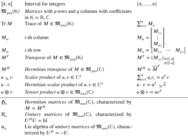
The notations given in Table 1 are used in this report.
3
Spectral clustering
The spectral clustering is performed through the following steps:
• We construct from 𝑛 data 𝑥1,… , 𝑥𝑛 a 𝑛 × 𝑛 matrix 𝐴 for which each entry 𝐴𝑖,𝑗 records a “similarity”
between 𝑥𝑖and 𝑥𝑗.
• Through a spectral embedding step, we transform the matrix 𝐴 into a 𝑘 × 𝑛 matrix 𝑌 that keeps the main features of 𝐴, where 𝑘 is the number of clusters, 𝑘 ⋘ 𝑛. This data reduction step uses the spectral information contained in 𝐴.
J𝑘, 𝑛K Interval for integers {𝑘, … , 𝑛} 𝔐𝑝×𝑞(𝕂) Matriceswith 𝑝 rows and 𝑞 columns with coefficients
in 𝕂 = ℝ, ℂ Tr 𝑀 Trace of 𝑀 ∈ 𝔐𝑛×𝑛(𝕂) ∑𝑛𝑖=1𝑀𝑖𝑖 𝑀∙𝑖 𝑖-th column 𝑀∙𝑖 = ⎡ ⎢ ⎢ ⎣ 𝑀1,𝑖 ⋮ 𝑀𝑛,𝑖 ⎤ ⎥ ⎥ ⎦ 𝑀𝑖∙ 𝑖-th row 𝑀𝑖∙ =[𝑀1,𝑖 ⋯ 𝑀𝑛,𝑖 ] 𝑀𝑇 Transposeof 𝑀 ∈ 𝔐 𝑝×𝑞(𝕂) 𝑀𝑇 = (𝑀𝑗,𝑖)𝑖∈J1,𝑝K 𝑗∈J1,𝑞K 𝑀𝐻 Hermitian transposeof 𝑀 ∈ 𝔐 𝑝×𝑛(ℂ) 𝑀 𝐻 = 𝑀𝑇 𝑢⋅ℝ𝑣 Scalar productof 𝑢, 𝑣 ∈ ℂ𝑑 ∑𝑑 𝑖=1𝑢𝑖𝑣𝑖 = 𝑢 𝑇𝑣
𝑢⋅ 𝑣 Hermitian scalar productof 𝑢, 𝑣 ∈ ℂ𝑑 𝑢⋅ 𝑣 = 𝑢𝑇 ⋅
ℝ𝑣
𝑢 ⊗ 𝑣 Tensor product 𝑢 ⊗ 𝑣∈ 𝔐𝑘×𝑛(ℂ) 𝑢 ⊗ 𝑣= 𝑢𝑣𝑇
ℌ𝑛 Hermitian matrices of 𝔐𝑛×𝑛(ℂ), characterized by
𝑀 = 𝑀𝐻
𝔘𝑛 Unitary matrices of 𝔐𝑛×𝑛(ℂ), characterized by
𝑈𝐻𝑈 = Id
𝔲𝑛 Lie algebra of unitary matrices of 𝔐𝑛×𝑛(ℂ), charac-terized by 𝑈𝐻 = −𝑈.
• We look for an orthogonal (if 𝐴 is symmetric) or unitary matrix 𝑈 whose axes encoding an orthonormal basis {𝑢1,… , 𝑢𝑘}on ℝ
𝑘or ℂ𝑘. This matrix is selected to minimaize the overall distance between the
columns vectors of 𝑌 , seen as elements of ℝ𝑘, and the rays emanating from 0 in one of the direction 𝑢 𝑖.
If the 𝑗-th column vector of 𝑌 is closest to the line in the direction 𝑢𝑖than in any other direction 𝑢𝓁, 𝓁 ∋,
then we assign the data 𝑥𝑗to the 𝑖-th cluster.
3.1 Dealing with asymmetric matrices
We consider a 𝑛 × 𝑛 matrix 𝐴 which is not necessarily symmetric. Lemma 1. The transform 𝐻 ∶ 𝔐𝑛×𝑛(ℝ) → ℌ𝑛defined by
𝐻(𝐴) = 1 2(𝐴 + 𝐴 𝑇 ) + 1 2𝑖(𝐴 − 𝐴 𝑇 )
is one-to-one with inverse 𝐻−1(𝑀) = ℜ𝑀 + ℑ𝑀 for 𝑀 ∈ ℌ𝑛.
As the matrix 𝐻(𝐴) is Hermitian, we may consider the eigenvalue problem
𝐻(𝐴)𝑥 = 𝜆𝑥, 𝑥 ∈ ℂ𝑑, 𝜆∈ ℝ.
The eigenvectors are orthogonal for the Hermitian scalar product. Therefore, we summarize the eigenvalue problem as
𝑉Λ𝑉𝐻 = 𝐻(𝐴) (1)
where 𝑉 is a unitary matrix and
Λ = ⎡ ⎢ ⎢ ⎣ 𝜆1 0 0 0 ⋱ 0 0 0 𝜆𝑑 ⎤ ⎥ ⎥ ⎦
with 𝜆1 ≥ … ≥ 𝜆𝑛. is a diagonal matrix containing the eigenvalues. The eigenvector of norm 1
corresponding to 𝜆𝑖is encoded into 𝑉∙𝑖.
3.2 Spectral embedding
The spectral embedding step consists in transforming the coordinates of the 𝑛 × 𝑛 matrix 𝐴 to a matrix 𝑌 of size 𝑘 × 𝑛, where 𝑘 is the number of clusters. This is a dimensension reduction.
Following [2], the package AsymmetricClustering considers by default the following spectral embedding princple. Other choices are possible [2, Table 3.2, p. 23].
Principle 1(Spectral embedding step). Using Λ and 𝑉 as in (1), we define
𝑌 = ⎡ ⎢ ⎢ ⎣ 𝜆−1∕2 1 0 0 0 ⋱ 0 0 0 𝜆−1∕2𝑘 ⎤ ⎥ ⎥ ⎦ [ 𝑉∙1 … 𝑉∙𝑘]𝐻 ∈ 𝔐𝑛×𝑘(ℂ).
As explained in [4], the spectral embedding step stems from the following principle: “Truncation of the eigenbasis amplifies any unevenness in the distribution of points on the 𝑑-dimensional hypersphere by causing points of high affinity to move toward each other and other to move apart.”
Remark1. With this matrix 𝑌 , we have 𝑌 𝑉∙𝑖=
{
𝜆−1∕2𝑖 if 1 ≤ 𝑖 ≤ 𝑘,
0 otherwise.
3.3 Transformation into an optimization problem The problem is now rewritten as an optimization problem.
Lemma 2. Given a point 𝑦 ∈ ℂ𝑘, 𝑛 ≥ 1 and a direction 𝑢 ∈ ℂ𝑘, the distance 𝑑(𝑦, 𝑢) between 𝑦 and its
orthogonal projection on 𝑢 is given by
𝑑(𝑦, 𝑢) = √
𝑦𝑇(Id −𝑢 ⊗ 𝑢)𝑦. (2)
Principle 2(General principle of spectral clustering). Given a matrix 𝑌 ∈ 𝔐𝑘×𝑛(ℂ), we consider finding a unitary matrix 𝑈 ∈ 𝔘𝑘×𝑘such that 𝑑(𝑌∙𝑖, 𝑈𝜎(𝑖))is minimal for each 𝑖 ∈J1, 𝑛K, where 𝜎 ∶ J1, 𝑛K → J1, 𝑘K. The cluster of the column 𝑖 is given by 𝜎(𝑖).
To set up Principle 2 in practive, we need to rewrite it by defining a cost function. For that, 𝜎 is replaced by 𝑊 ∈ 𝔐𝑘×𝑛containing exactly one and only one 1 on each row. The cost function1 is
𝐽(𝑌 , 𝑈 , 𝑊 ) = 𝑛 ∑ 𝑖=1 𝑘 ∑ 𝑗=1 𝑊𝑗,𝑖𝐷𝑗,𝑖with 𝐷𝑗,𝑖 = 𝑑(𝑌∙𝑖, 𝑈∙𝑗)2 (3) for 𝑌 ∈ 𝔐𝑘×𝑛(ℂ), 𝑈 ∈ 𝔘𝑘×𝑘and 𝑊 ∈ 𝔐𝑘×𝑛(ℝ)with the constraint
𝑊𝑗,𝑖 ∈ {0, 1}and
𝑘
∑
𝑗=1
𝑊𝑗,𝑖= 1for 𝑖 = 1, … , 𝑛. (4)
Principle 3. Fix 1 ≤ 𝑘 ≤ 𝑛. Given 𝑌 ∈ 𝔐𝑘,𝑛(ℝ), find 𝑈 ∈ 𝔐𝑘×𝑘(ℂ)and 𝑊 ∈ 𝔐𝑘×𝑛(ℝ)satisfying (4) such that
𝐽(𝑌 , 𝑈 , 𝑊 )is minimal with 𝑈 ∈ 𝔘𝑘 and 𝑊 satisfies (4).
(5) The constraint (4) is relaxed into
0≤ 𝑊𝑖,𝑗 ≤ 1 and
𝑘
∑
𝑗=1
𝑊𝑗,𝑖 = 1for 𝑖 = 1, … , 𝑛. (6)
We coefficients 𝑊𝑖,𝑗 are then seen as weights that quantify the probability to belong to a class 𝑘.
Principle 4(Minimization of the cost function, relaxed version of Principle 3). Fix 1 ≤ 𝑘 ≤ 𝑛. Given
𝑌 ∈ 𝔐𝑘,𝑛(ℝ), find 𝑈 ∈ 𝔐𝑘×𝑘(ℂ)and 𝑊 ∈ 𝔐𝑘×𝑛(ℝ)satisfying (4) such that
𝐽(𝑌 , 𝑈 , 𝑊 )is minimal with 𝑈 ∈ 𝔘𝑘 and 𝑊 satisfies (6).
(7) The cluster for the column 𝑖 of 𝑌 is given by arg max1≤𝑗≤𝑘𝑊𝑗,𝑖
The minimization problem 7 is solved using an iterative approach in which we alternatively optimize over the weights and over unitary matrices, up to reaching a state in which the update are small. A “temperature” parameter is updated at each global step.
4
Numerical algorithms
4.1 Algorithm 1: updating the weights
When 𝑈 is fixed, the weight matrix 𝑊 is updated through
𝑊𝑗,𝑖(𝜎, 𝑌 , 𝑈 ) = ∑ exp(−𝐷𝑗,𝑖∕𝜎)
𝑘
𝓁=1exp(−𝐷𝓁,𝑖∕𝜎)
for 𝑗 ∈J1, 𝑘K, 𝑖 ∈ J1, 𝑛K,
with 𝐷𝑗,𝑖 = 𝑑(𝑌∙𝑖, 𝑈∙𝑗)2 (see (3)) for a scale parameter 𝜎. Thus, the column 𝑊∙,𝑖is the output the softmax
function ⎛ ⎜ ⎜ ⎝ ⎡ ⎢ ⎢ ⎣ 𝑥1 ⋮ 𝑥𝑘 ⎤ ⎥ ⎥ ⎦ , 𝜎 ⎞ ⎟ ⎟ ⎠ = ∑ 1 𝑘 𝑖=1exp(𝑥𝑖∕𝜎) ⎛ ⎜ ⎜ ⎝ ⎡ ⎢ ⎢ ⎣ exp(𝑥1∕𝜎) ⋮ exp(𝑥𝑘∕𝜎) ⎤ ⎥ ⎥ ⎦ ⎞ ⎟ ⎟ ⎠ ,
applied to the vector 𝐷∙,𝑖. The function 𝜎 ↦ 𝐽(𝑌 , 𝑈, 𝑊 (𝜎, 𝑌 , 𝑈)) is non-decreasing. Reducing 𝜎 reduces
the cost function. At the end of the 𝑚-th step, we update the scale parameter 𝜎 as
𝜎𝑚+1 = 𝐽(𝑌 , 𝑈𝑚, 𝑊(𝜎𝑚, 𝑌 , 𝑈𝑚))
𝑛⋅ 𝑚 .
To avoid numerical problems with the softmax function , we actually use the formula ⎛ ⎜ ⎜ ⎝ ⎡ ⎢ ⎢ ⎣ 𝑥1 ⋮ 𝑥𝑘 ⎤ ⎥ ⎥ ⎦ , 𝜎 ⎞ ⎟ ⎟ ⎠ = ∑ 1 𝑘 𝑖=1exp ( 𝑥𝑖−𝑚 𝜎 ) ⎛ ⎜ ⎜ ⎜ ⎝ ⎡ ⎢ ⎢ ⎢ ⎣ exp ( 𝑥1−𝑚 𝜎 ) ⋮ exp ( 𝑥𝑘−𝑚 𝜎 ) ⎤ ⎥ ⎥ ⎥ ⎦ ⎞ ⎟ ⎟ ⎟ ⎠ with 𝑚 = max 𝑗=1,…,𝑘𝑥𝑗.
See [3] for numerical considerations on the computation of the softmax function. 4.2 Algorithm 2: minimization over the unitary matrices
During this optimisation step, the matrix 𝑊 is fixed. The problem is then to optimize over unitary matrices. For this, a conjugate gradient method is used in the framework of a Riemannian algorithm [5] that takes profits from the geometry of the Lie group of unitary matrices. The algorithm implements the method of [1].
At each point 𝑈 of 𝔘𝑛, the tangent space 𝑇𝑈 𝔘𝑛is the set
𝑇𝑈 𝔘𝑛 = {𝑆𝑈 | 𝑆 ∈ 𝔲𝑛}with 𝔲𝑛 = {𝑆 ∈ 𝔐𝑛× 𝑛(ℂ)| 𝑆𝐻 = −𝑆}. The tangent space is also identified with the set
𝑇𝑈𝔘𝑛 = {𝑆 ∈ 𝔐𝑛×𝑛(ℂ)| 𝑈
𝐻𝑆
+ 𝑆𝐻𝑈 = 0}. On 𝔐𝑛×𝑛(ℂ), we define a scalar product as
⟪𝑀, 𝑁⟫ = 1
2ℜ Tr(𝑀𝑁
𝐻
). Lemma 3. For 𝑀 ∈ 𝔐𝑛×𝑛(ℂ), write 𝑀a = 1
2(𝑀 − 𝑀
𝐻). The map 𝑝⊥ ∶ 𝑀 ↦ 𝑀
a is the orthogonal
Proof. For this scalar product, Hermitian and anti-Hermitian matrices are orthogonal. Any matrix 𝑀
is decomposed as 𝑀 = 𝑀s+ 𝑀a with 𝑀s = 1
2(𝑀 + 𝑀
𝐻)which is Hermitian and 𝑀
a which is
anti-Hermitian.
As any element of 𝑇𝑈 𝔘𝑛is writen 𝑆𝑈 for some 𝑆 ∈ 𝔲𝑛and 𝑈−1 = 𝑈∗, a scalar product is naturally on
𝑇𝑈𝔘𝑛 for any 𝑈 ∈ 𝔘𝑛 as
⟨𝑉 , 𝑊 ⟩𝑈 =⟪𝑉 𝑈
−1, 𝑊 𝑈−1⟫ = 1
2ℜ Tr(𝑉 𝑈
𝐻𝑈 𝑊𝐻) =⟪𝑉 , 𝑊 ⟫.
This way, ⟨⋅, ⋅⟩ gives rise to a Riemannian metric.
Lemma 4. The orthogonal projection of 𝑀 ∈ 𝔐𝑛×𝑛(ℂ) onto 𝑇𝑈𝔘 for 𝑈 ∈ 𝔘𝑛is
𝑝⊥𝑈(𝑀) = 𝑀 − 𝑈 𝑀𝐻𝑈 . (8)
Proof. We set 𝑝⊥
𝑈 ∶ 𝑀 ↦ 𝑝
⊥(𝑀𝑈−1)𝑈. It is easily checked that ⟨𝑝⊥
𝑈(𝑀), 𝑊⟩𝑈 = 0for any 𝑊 ∈ 𝑊 ∈
𝑇𝑈𝔘𝑛. Using Lemma 3, this leads to (8).
The geodesics emanating from 𝑈 in the direction 𝑆𝑈 ∈ 𝑇𝑈 𝔘𝑛, that is for 𝑆 ∈ 𝔲𝑛, are then
𝛾(𝑡) = exp(𝑡𝑆)𝑈 where 𝑆 ↦ exp(𝑆) is the matrix exponential.
Gradients are computed with respect to the complex conjugate derivative operator
𝜕 𝜕𝑈𝐻 = 1 2 ( 𝜕 𝜕ℜ𝑈 + i 𝜕 𝜕ℑ𝑈 ) .
The Riemannian gradient of 𝑓 ∶ 𝔘𝑛 → ℝat 𝑈 is the orthogonal projection of 𝜕𝑓 𝜕𝑈𝐻 onto 𝑇𝑈𝔘𝑛, so that with (8), ∇𝔘𝑓(𝑈 ) = 𝜕𝑓 𝜕𝑈𝐻 − 𝑈 ( 𝜕𝑓 𝜕𝑈𝐻 )𝐻 𝑈 . (9)
4.2.1 The conjugate gradient
Notation 1. The gradient of the cost function 𝐽(𝑌 , 𝑈, 𝑊 ) at point 𝑈 ∈ 𝔘𝑛is denoted by Γ(𝑈) = 𝜕𝐽(𝑌 ,𝑈 ,𝑊 )
𝜕𝑈𝐻 .
The conjugate gradient algorithm consists in finding successive points 𝑈𝑘in 𝔘𝑛by
• At 𝑈𝑘, the next point 𝑈𝑘+1is computed by following the geodesic through a search direction −𝐻𝑘 ∈
𝑇𝑈
𝑘𝔘𝑛, as
𝑈𝑘+1 = exp(−𝜇𝐻𝑘)𝑈𝑘with 𝜇 = arg min 𝐽(𝑌 , exp(−𝜇𝐻𝑘)𝑈𝑘, 𝑊). The scalar 𝜇 is choosen according to a line search algorithm presented in § 4.2.3.
• At 𝑈𝑘+1, the search direction is updated by combining the direction given by steepest descent gradient
𝐺𝑘+1 = Γ(𝑈𝑘+1)𝑈𝑘𝐻+1− 𝑈𝑘+1Γ(𝑈𝑘)𝐻
and 𝐻𝑘. As 𝐺𝑘+1 ∈ 𝑇𝑈𝑘+1𝔘𝑛and 𝐻𝑘 ∈ 𝑈𝑇𝑘𝔘𝑛, 𝐻𝑘a parallel transport is used, so that 𝐻𝑘is transformed
into
̃
The new search direction is defined so that
− 𝐻𝑘+1 = −𝐺𝑘+1− 𝜃 ̃𝐻𝑘 (10)
where 𝜃 is selected so that 𝐻𝑘+1 and ̃𝐻𝑘are Hessian conjugate, that is
𝐻𝑘𝑇+1Hess 𝐽 (𝑌 , 𝑈𝑘+1, 𝑊) ̃𝐻𝑘 = 0.
The value of 𝜃 is actually computed using the Polak-Ribière approximation [1, Eq. (10), § 2.4],
𝜃= ℜ Tr((𝐺𝑘+1− 𝐺𝑘) 𝐻𝐺 𝑘+1) ℜ Tr 𝐺𝐻 𝑘 𝐺𝑘 . (11) 4.2.2 The gradient
Let us compute first the gradient of the distance 𝑑(𝑦, 𝑢)2given by (2) for two vectors 𝑦 and 𝑢 in ℂ𝑘. We
note first that
𝜕𝑢𝑖 𝜕𝑢𝐻𝑖 = 0for 𝑖 ≠ 𝑗, 𝜕𝑢𝑗 𝜕𝑢𝐻𝑖 = 1for 𝑖 ≠ 𝑗 and 𝜕𝑢𝑖𝑢𝑖 𝜕𝑢𝐻𝑖 = 𝑢𝑖. Therefore, 𝜕𝑑(𝑦, 𝑢)2 𝜕𝑢𝐻 𝑖 = − 𝑘 ∑ 𝑝=1 𝑦𝑝𝑢𝑝𝑦𝑖 = −(𝑦𝐻 ⋅ 𝑢)𝑦𝑖.
Applied to the cost function,
𝜕𝐽(𝑌 , 𝑈 , 𝑊 ) 𝜕𝑈𝐻 𝑟,𝑐 = − 𝑛 ∑ 𝑖=1 𝑊𝑐,𝑖((𝑌∙𝑖)𝐻 ⋅ 𝑈∙𝑐)𝑌𝑟,𝑖 = − 𝑛 ∑ 𝑖=1 𝑘 ∑ 𝑗=1 𝑊𝑐,𝑖(𝑌𝐻𝑈)𝑖,𝑐𝑌𝑟,𝑖.
4.2.3 The line search
The line search algorithm consists in finding the minimal point of the cost function along a geodesic curve. More precisely, of
𝐺(𝜇) = 𝐽 (𝑌 , exp(−𝜇𝐻)𝑈 , 𝑊 )
for a direction 𝐻 ∈ 𝔲𝑛, as 𝜇 ↦ exp(−𝜇𝐻)𝑈 is a geodesic passing through 𝑈 in the direction 𝐻𝑈.
Here, 𝐻 is the search direction: it is either the steepest descent (computed from the Riemannian Gradient ∇𝔘𝐽(𝑌 , 𝑈 , 𝑊 )) given by (9)) or the conjugate gradient (see (10) and (11)).
We rewrite
𝐺(𝜇) = 𝐽 (𝑌 , (1 + 𝑍)𝑈 , 𝑊 )with 𝑍 = exp(−𝜇𝐻) − 1.
The cost function 𝐽 is quadratic in 𝑈, so that there exists 𝐽1linear and 𝐽2bilinear on 𝔐𝑘×𝑘(ℂ)such that
𝐺(𝜇) = 𝐺(0) + 𝐽1⋅ (exp(−𝜇𝐻) − 1) + 𝐽2⋅ (exp(−𝜇𝐻) − 1) ⊗ (exp(−𝜇𝐻) − 1). (12) Let us recall a standard result on the spectral decomposition of anti-Hermitian matrices.
Lemma 5. The spectrum of 𝐻 is purely imaginary, so thatexp(−𝜇𝐻) = 𝑄 Diag(𝑒−𝜇i𝜔1,… , 𝑒−𝜇i𝜔𝑘)𝑄𝐻
It follows from the above property and (12) that 𝐺(𝜇) is the linear superposition of function of type
𝜇 ↦exp(−𝜇i𝜔𝑗)and 𝜇 ↦ exp(−2𝜈i𝜔𝑗).
With 𝜔 = max𝑖=1,…,𝑘|𝜔𝑖|, we then restrict the search of the minimum of 𝐺(𝜇) to the interval [0, 2𝜋∕𝑞𝜔]
with 𝑞 = 2, as 𝐺(𝜇 + 2𝜋𝜔) is close to 𝐺(𝜇).
With the chain rule and the definition of the Riemannian gradient,
𝐺′(𝜇) = −2ℜ Tr(∇𝔘𝐽(𝑌 , exp(−𝜇𝐻)𝑈 , 𝑊 )𝑈𝐻exp(−𝜇𝐻)𝐻𝐻𝐻)
since the derivative of 𝜇 ↦ exp(−𝜇𝐻)𝑈 is 𝐻 exp(−𝜇𝐻)𝑈 ∈ 𝑇exp(−𝜇𝐻)𝑈𝔘𝑛.
As the search direction imposes that 𝐺′(0) < 0, to find the minimum of 𝐺(𝜇), we look for the smallest
zero-crossing of the derivative.
To avoid the high cost of computing the exponential exp(−𝜇𝐻) too frequently, we use a polynomial approximation of 𝐺′(𝜇). Thus, 𝐺′(𝜇)is evaluated at the 𝑃 spaced point 𝜇
𝑘 = 𝑘𝜋
𝑃 𝜔, 𝑘 = 1, … , 𝑃 . Hence,
exp(−𝜇𝑘𝐺) = exp(−𝜇1𝐺)𝑘 for 𝑘 = 1, … , 𝑃 .
With the approximation
𝐺′(𝜇) ≈ 𝐺′(0) + 𝑃 ∑ 𝑘=1 𝑎𝑘𝜇𝑘, we obtain 𝐺′(𝜇𝑖) ≈ 𝐺′(0) + 𝑃 ∑ 𝑘=1 𝑎𝑘𝜇𝑖𝑘for 𝑖 = 1, … , 𝑃 .
The 𝑎𝑖are then found by solving the linear system
⎡ ⎢ ⎢ ⎣ 𝐺′(𝜇1) − 𝐺′(0) ⋮ 𝐺′(𝜇𝑃) − 𝐺′(0) ⎤ ⎥ ⎥ ⎦ = ⎡ ⎢ ⎢ ⎣ 𝜇1 ⋯ 𝜇𝑃 1 ⋮ ⋮ ⋮ 𝜇𝑘 ⋯ 𝜇𝑃 𝑘 ⎤ ⎥ ⎥ ⎦ ⎡ ⎢ ⎢ ⎣ 𝑎1 ⋮ 𝑎𝑃 ⎤ ⎥ ⎥ ⎦ .
The line search algorithm returns the smallest positive root of 𝑎0 + 𝑎1𝜇 + ⋯ + 𝑎𝑃𝜇𝑃 = 0if it exist.
Otherwise, it returns 0, and a new direction is computed.
References
[1] T. Abrudan, J. Eriksson, and V. Koivunen. “Conjugate gradient algorithm for optimization under unitary matrix constraint”. In: Signal Processing 89.9 (Sept. 2009), pp. 1704–1714.DOI: 10.1016/
j.sigpro.2009.03.015.
[2] S. E. Atev. “Using Asymmetry in the Spectral Clustering of Trajectories”. University of Minnesota, 2011.
[3] P. Blanchard, D. J. Higham, and N. J. Higham. Accurate Computation of the Log-Sum-Exp and
Softmax Functions. 2019. arXiv: 1909.03469.
[4] M. Brand and K. Huang. “A unifying theorem for spectral embedding and clustering”. In: AISTATS. 2003.
[5] A. Edelman, T. A. Arias, and S. T. Smith. “The Geometry of Algorithms with Orthogonality Con-straints”. In: SIAM Journal on Matrix Analysis and Applications 20.2 (Jan. 1998), pp. 303–353.DOI:
10.1137/s0895479895290954.
[6] U. von Luxburg. “A tutorial on spectral clustering”. In: Statistics and Computing 17.4 (Dec. 2007), pp. 395–416.DOI: 10.1007/s11222-007-9033-z.