A unifying framework for specifying DEVS parallel and distributed simulation architectures

HAL Id: hal-01814164

https://hal.archives-ouvertes.fr/hal-01814164

HAL is a multi-disciplinary open access

archive for the deposit and dissemination of sci-entific research documents, whether they are pub-lished or not. The documents may come from teaching and research institutions in France or abroad, or from public or private research centers.

L’archive ouverte pluridisciplinaire HAL, est destinée au dépôt et à la diffusion de documents scientifiques de niveau recherche, publiés ou non, émanant des établissements d’enseignement et de recherche français ou étrangers, des laboratoires publics ou privés.

A unifying framework for specifying DEVS parallel and

distributed simulation architectures

Adedoyin Adegoke, Hamidou Togo, Mamadou Kaba Traoré

To cite this version:

Adedoyin Adegoke, Hamidou Togo, Mamadou Kaba Traoré. A unifying framework for specifying DEVS parallel and distributed simulation architectures. SIMULATION, SAGE Publications, 2013, 89 (11), pp.1293-1309. �10.1177/0037549713504983�. �hal-01814164�

A Unifying Framework for Specifying DEVS Parallel and Distributed

Simulation Architectures

(1) African University of Science and Technology, Abuja (Nigeria) (2) Université des Sciences, Techniques et Technologies de Bamako (Mali) (3) LIMOS, CNRS UMR 6158, Université Blaise Pascal, Clermont-Ferrand 2 (France)

Abstract

DEVS (Discrete Event System Specification) is an approach in the area of Modeling and Simulation (M&S) that provides a means of specifying dynamic systems. A variety of DEVS tools have been implemented without a standard developmental guideline across the board consequently revealing a lack of central frameworks for integrating heterogeneous DEVS simulators. When implementing a DEVS Simulator there are salient concepts that are intuitively defined like how events should be processed, what simulation architecture to use, what existing procedures (set of rules/algorithm) can be used, what should be the organizational architecture and so on. The aim of this paper is to propose a theoretical guide in building a DEVS distributed simulation as well as a formalization of underlying concepts to allow symbolic reasoning and automated code synthesis. From a review of existing implementation approaches, we propose a taxonomy of the identified concepts including some formal definitions as they constitute the essential building blocks of performing Parallel Discrete-Event Simulation (PDES) by utilizing DEVS. The contribution of this taxonomy and its impact as a unifying framework is that it provides a more systematic understanding of the process of constructing a DEVS simulator. Also, it offers an abstract way for integrating different and heterogeneous DEVS implementation strategies and thus can serve as a contribution to the on-going DEVS standardization efforts.

1. INTRODUCTION

DEVS (Discrete Events Systems Specification) offers a platform for the modeling and simulation of sophisticated systems in a variety of domains. It provides a mechanism to mix different formalisms as well as a generic mechanism for modeling and simulation. A DEVS simulator is capable of reproducing behaviors that are identical to that of the system under observation. In doing so, the modeler is provided with some level of abstraction by being able to build models without having knowledge of how the simulator was built.

Due to the growing complexity of systems to be modeled, efficient simulation of such systems cannot be performed on a single physical processor. One way out of this is to make use of distributed strategies by exploiting the computing power of current technologies (grid, cloud, web services etc.). Some benefits of this include: reduction in execution time, improved simulation performance, real time execution and integration of simulators [1]. Parallel Discrete-Event Simulation (PDES) [1] has been a widely researched area with some potential benefits. First, the use of parallel processors promises an increase in execution speed and a reduction in execution time. Second, the potentially larger amount of available memory on parallel processors will enable the execution of larger simulation models. Third, with the use of multiple processors comes an increased tolerance to a possible processor failure. In addition, it provides a solution to the scientific need to federate existing and naturally dispersed simulation codes. Thus, simulation architecture can be called parallel if its main design goal is to reduce execution time while the term distributed simulation could be referred to as interoperating geographically dispersed simulators [1, 2, 3]. Building a simulation model on a particular world view significantly reduces implementation complexity [4]. However, the distribution

of the DEVS simulation protocol (which unifies the three classic simulation strategies also known as the world views [2]) is a challenging issue.

PDES is a matured field of study but its adaptability to some existing modeling and simulation formalisms (e.g., DEVS or Petri nets) is an arduous task. Two main reasons concur to this point:

• Various concerns are involved in the process of building a DEVS PDES. A good building strategy would be based on a clear separation of concerns. The formal specification of the key concepts and transformation that are found in these concerns would remove ambiguity and reduce accidental complexity (i.e., wrong implementation due to misunderstanding of concepts).

• There is a lack of systematic and quantifiable approach that can guide this process.

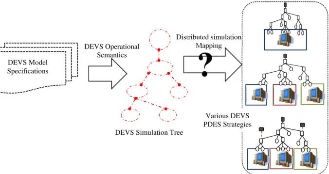
DEVS simulation principle takes a DEVS model specification and maps it to DEVS simulation tree using well-defined DEVS operational semantics [2]. From studied literature it is seen that most works are moving from sequential to parallel/distributed infrastructures due to the benefits involved in so doing. Also from this study we see the existence of various DEVS PDES strategies (as shown in Figure 1). However this raises the question of how we can achieve the mapping of a DEVS simulation tree onto parallel/distributed infrastructures. The objective of this work is to:

• Propose a conceptual framework that models the process of mapping DEVS simulation tree to a graph of simulation components distributed over a network. Then, each builder of DEVS distributed simulation can instantiate this generic model to get his own mapping strategy which, therefore is a guideline for any user to apply this strategy.

• Formalize the concepts and operations of such a process so that: 1. There can be the partial or full automation of such a process.

2. One can symbolically reason and derive properties (for evaluation or verification). The rest of the paper is organized as follows: Section 2 presents the foundations of DEVS simulation, i.e., the simulation tree, from which all the distributed strategies are built. Section 3 presents the key concepts in use in this paper. Identified aspects in DEVS PDES as well as classification of research contributions in this area are presented in Section 4. In Section 5 we present the generic approach for building a DEVS PDES implementation and we show how it instantiates in a case study. In Sections 6, we give a discussion on the framework and then conclude in Section 7.

Figure 1: Process of mapping DEVS to PDES Distributed simulation

Mapping DEVS Model

Specifications

DEVS Simulation Tree DEVS Operational

Semantics

?

Various DEVS PDES Strategies

2. DEVS SIMULATION PROTOCOL

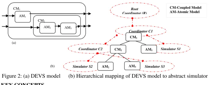
The DEVS formalism [2] provides a comprehensive modeling and simulation framework for modeling and analysis of Discrete Event Systems. It specifies system behavior as well as system structure. System behavior in DEVS is described through its DEVS dynamic functions while system structure is built from the composition of atomic and coupled models. A coupled model is composed of several atomic or coupled models and atomic model is a basic component that cannot be decomposed any further. They are hierarchically organized as shown in Figure 2.a.

A DEVS model is built according to specification, i.e., Classic DEVS (CDEVS) or Parallel DEVS (PDEVS). CDEVS was introduced in 1976 by Zeigler [5] to simulate and execute models sequentially on single processor machine. PDEVS has later been introduced to increase the potential of parallelism in simulating DEVS models [6].

Due to the separation of concerns in DEVS, the modeler needs to focus only on the models being created avoiding the details about the abstract simulator (algorithms). The operational semantics of DEVS models has been defined by abstract algorithms [2]. These algorithms consist of different Nodes (Coordinator, Simulator) organized in a hierarchy that mimics the hierarchical structure of a model. In these algorithms, a DEVS atomic model is executed by assigning a simulator to it and to a DEVS coupled model a coordinator is assigned. From its original definition, the DEVS abstract simulator structure is hierarchical in nature and the hierarchy of models is mapped onto it (Figure 2.b). The distinctiveness of the DEVS framework is in its hierarchical compositional structures which help in complexity reduction. During simulation, the interaction/communication between different model components is achieved through event messages exchanged between the Simulators and Coordinators, each representing an event to be processed.

Two key information carried by these messages are their category and timestamp. The category of a message is associated to a certain form of treatment the receiver component (Coordinator or Simulator) must perform. The timestamp indicates the simulation time this message has been generated.

In CDEVS [5], categories are *, i, x, and y. In the first version of PDEVS [6], categories are *, i, q, done, @, and y. Next versions propose various sets of categories (with associated set of treatments). However, all DEVS-based algorithms adhere to the same simulation principle (i.e., generalized or specialized Coordinators and Simulators exchanging messages and performing specific actions on receipt of specific categories of message).

Figure 2: (a) DEVS model (b) Hierarchical mapping of DEVS model to abstract simulator

3. KEY CONCEPTS

In this section we briefly introduce key concepts of the framework. They are:

• Root Coordinator: it is the simulating element that manages the time of a simulation tree.

• Nodes: They are simulation entities used for executing DEVS models. These nodes are Coordinators, Simulators and Root Coordinators. The Root Coordinator has an event loop

(a) CM1 AM1 CM2 AM2 AM3 CM-Coupled Model AM-Atomic Model Root Coordinator (R) Coordinator C2 CM2 AM1 Simulator S1 Simulator S2 AM2 AM3 Simulator S3 Coordinator C1 CM1 (b)

which sends event messages and controls the simulation cycles while the Coordinator and Simulator are capable of receiving, treating and sending event messages.

• Simulation Tree: A tree is made up of nodes. The Root Coordinator is always at the top of the Tree’s hierarchy and has a Coordinator as its descendant. Also, the Coordinator has either a Coordinator or Simulator as its descendant but the Simulator has none.

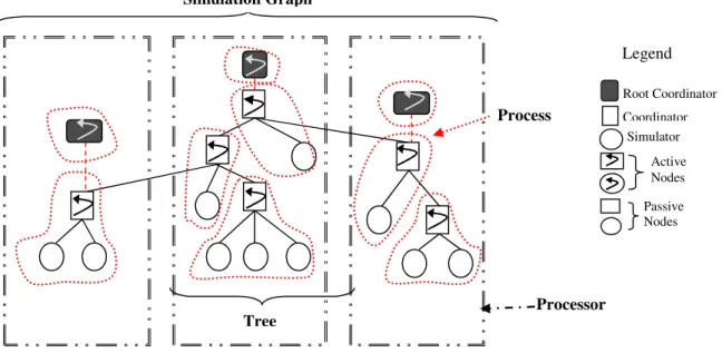
• Process: We define it as a stream of execution. It contains two types of nodes during execution; they are active and passive nodes. An active node is a node that is currently active in an execution stream (e.g., Java threads or ADA tasks). While a passive node is part of an execution stream but not actively involved until it is triggered (e.g., function calling in Object Oriented Paradigm). We consider that a process would have at most one active node. If a process has more than one active node, those nodes are then regarded as being autonomous sub-processes. Also, there can be more than one passive node in a process.

• Activity: Set of actions that are performed at the receipt of an event.

• Processor: Computing resource that allows the execution of a program (a process, an entire tree, any other executable code) on itself.

• Simulation Graph: A representation of the relationship between the identified aspects in DEVS simulation. An example of Simulation Graph can be seen in Figure 3. Details about its components are discussed in the following sections.

We also formalize these concepts. Numerous formal definitions are given throughout the paper for the following reasons:

• They provide a clear understanding (by reducing ambiguity) of simulation structures and operations we introduce. We use definitions given in earlier sections to formalize concepts presented in later sections.

• They provide mathematical objects that one can use for consistency checking or validity checking.

• They can ease the automation of processes defined with them.

Definitions 1 and 2 given below will be used as building blocks to formalize simulation structures we’ll introduce later, as well as the generic operations that make up the framework. Although they are equivalent, one or the other definition is more convenient to use in specifying other concepts.

Definition 1: We formally define Simulation Tree as T = <R, N, f> With:

• R

∈

• f: N →

℘

℘

∅

• f-1_(J)

≠

∅

∀

∈

Where:

R: The Root Coordinator of the tree N: The set of nodes of the tree

f: A function that maps a child node to its parent (the one at one step higher in the hierarchy).

For example, the tree given in Figure 2.b is defined as T = <R, {R, C1, C2, S1, S2, S3}, f>, where f(R) = {C1}, f(C1) = {C2, S1}, f(C2) = {S2, S3}, and f(S1) = f(S2) = f(S3) = ∅

Definition 2: Simulation Tree can also be defined as T = <R, N, F> With:

• R

∈

• F

⊂

×

∈

⇔

∈

Using Definition 2 for the example of Figure 2.b, and will be defined as same while will be {(R, C1), (C1, C2), (C1, S1), (C2, S2), (C2, S3)}

Figure 3: Relationship between Trees, Processes and Processors in a Graph

4. TAXONOMY IN DEVS PARALLEL AND DISTRIBUTED SIMULATION

There are different practices behind the concept of exploiting DEVS with PDES. Due to this, the concept becomes burdened with variances in opinions on how to build a DEVS simulator. We were able to identify four major factors in use in these practices. First, some approaches alter the tree structure [3, 7, 8, 9, 10, 11, 12, 13]. We call this “Tree Transformation”. Second, most approaches split the model tree into many trees [14, 15, 16, 17]. We call this “Tree-Splitting”. Also, some approaches differ on the number of executions/processes that can be performed per simulation run [19]. We call this “Node-Clustering”. Lastly, some approaches vary the number of computing resources to be used during simulation [2, 11]. We call this “Process-Distribution. In the following sections we present and formalize these concepts. Doing so, we also offer a review of major strategies proposed in the literature.

4.1. Tree Transformation

It has been observed that altering a simulation tree structure can improve simulation performance and also enhance distribution. This transformation is usually achieved either by reducing or increasing the number of nodes of a tree.

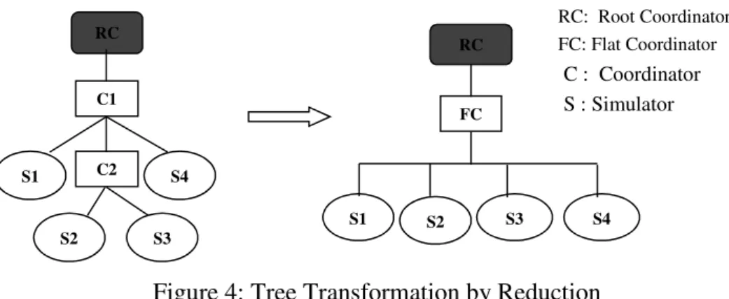
4.1.1. Reduction

As presented in [7] the hierarchical structure of the simulator (which has a one-to-one correspondence with the DEVS model architecture) can increase the communication overhead between Nodes. The process of reducing the number of these nodes on a tree is also known as flattening. A flattened simulator [8] simplifies the hierarchical simulator while keeping a hierarchical model structure (see Figure 4). Various studies [9, 10] have shown that a flattened simulator reduces these costs. CD++ uses a flat simulation approach that eliminates the need for intermediate coordinators to improve the performance of simulation [3, 12]. Some other approaches prefer to alter the compositional structure of a DEVS model. Kim proposed transforming a hierarchical DEVS model into a non-hierarchical structure to ease synchronization in a distributed simulation [11]. Zeigler also considered building Conservative DEVS simulator for non-hierarchical models [2].

Simulation Graph Processor Process Tree Root Coordinator Simulator Coordinator Active Nodes Passive Nodes Legend

Figure 4: Tree Transformation by Reduction

4.1.2. Expansion

In [13] the expansion was achieved by introducing new simulation nodes into the simulation tree structure as presented in Figure 5. This is to enable the distribution of nodes on different processors. The introduction of extra components on the tree introduces more concerns as to what type of information each of these new components should contain. Also, communication between these Nodes constitutes an increasing overhead cost as the structure of the messages being passed is altered to accommodate extra information. For example a new sub-coordinator has no coupled model associated with it and therefore contains no coupling information. Also, it has to correctly identify imminent models and influencees. One way to deal with this is through the composition of messages, i.e., by including more information in a message’s construct, as seen in [13]. In PCD++ [24, 25], the inclusion of Node Coordinators in the simulation tree was to enable synchronization and communication between processes in a distributed environment.

Figure 5: Tree Transformation by Expansion

4.1.3. Formal Specification for Tree Transformation

Definition 3:Σ = ⋃ _∈ X ∪ (⋃ _∈ Y ) ∪ (R ∪ 0, +∞ ) Formally we define Tree

Transformation as

Transf[Na,Nr,Fa,Fr]: τ → τ where τ is the set of all possible simulation trees

Transf[Na,Nr,Fa,Fr](<R, N, F>) = <R’, N’, F’> With

• N’ = N

∪

∪

• Na is the set of nodes to be added to

• Nr is the set of nodes to be removed from

• Fa is the set of relationships to be added to

• Fr is the set of relationships to be removed from

Based on the following conditions:

• Na

∩

∅

RC C1 C2 _S4 S3 S2 S1 RC FC S3 S1 S2 S4 RC: Root Coordinator FC: Flat Coordinator C : Coordinator S : Simulator RC C S3 S1 S2 S4 RC C S3 S4 C*2 S1 S2 C*1 C* : New Coordinator

• Nr

⊂

• Fa

⊂

×

∪

∪

×

• Fr

⊆

Tree splitting can be referred to as the decomposition of a simulator tree to form sub-trees based on the analysis of the model’s structure. We identified two types namely, single tree structure and multiple tree structure. It is necessary to state here that this section does not deal with how the tree structure can be split or executed, or how they can be mapped to available number of processors.

4.2.1. Single Tree Structure

In describing this structure, executing a model with a single tree structure can be expressed as having an entire model tree simulated with the use of a central scheduler called the Root Coordinator. Single tree structures are mostly implemented using CDEVS and PDEVS algorithms. In CDEVS [2] events are processed in a sequence. This approach is the simplest form of simulation but it does not properly reflect the simultaneous occurrence of events in the system being modeled. Indeed, serialization reduces possible utilization of parallelism during the occurrence of events. On the other hand, Chow and Zeigler [6] introduced PDEVS as a possible solution to the problem of serialization. According to Chow, one desirable property provided by PDEVS is the degree of parallelism which can be exploited in parallel and distributed simulation. It beats the restrictions in CDEVS in both execution time and memory usage.

4.2.2. Multiple Trees

We look at the multiple tree structure as when a tree can be split into different sub-trees with each having its own central scheduler/Root Coordinator and different simulation clocks. This is the preferable solution in distributed simulation. Based on this structure, all events with the same timestamp are scheduled to be processed simultaneously. Distributed simulation algorithms are used to synchronize trees.

The two basic distributed simulation algorithms in use are the Optimistic [17] and Conservative (Pessimistic) [14, 15, 16] algorithms. Optimistic algorithms, in contrast to Conservative algorithms, enable increased degrees of parallelism. However, they also result in more complex algorithms. Communication between these trees is usually between:

a. Root Coordinator and Root Coordinator (see Figure 6a), e.g., DEVS Time Warp [2]. b. Coordinators and Simulators (Parents and their Children in the initial tree), e.g.,

DOHS scheme [7] (see Figure 6b)

a) Communication between Root b) Communication between Coordinators Figure 6: Communication schemes between tree structures

4.2.3. Formal Specification for Tree Splitting Definition 4: Formally we define Tree Splitting as

Split:τ → Σ Split(<R, N, f>) = <{Ri}, N’, f’> Where Communication Parenthood in the initial Simulation Tree

• Σ is the set of all simulation skeletons (see the definition of this structure in section 5)

• R

∈

• N’ = N

∪

• f’/N = f

4.3. Node Clustering

This is the association of one or many nodes to various processes. Events execution is driven through the use of processes. We take a look at the concept of process as an execution stream. A process can be seen as a mechanism that is able to execute events. We categorize based on the number of processes: as “one process” execution or “many processes” execution. However, we will not be dealing with how execution takes place on processors.

4.3.1. One Process

A one-process execution denotes having events processed in a serially and orderly manner, i.e., one after another. This restricts concurrent execution streams. In [18] the authors denote this form of execution as “sequentialization”. In this sense, for example, the “main” program is a process. A desired speed up may not be achieved when using a one-process execution stream. On the other hand, it is easier and faster to implement. During the one-process execution, interaction between the nodes is called intra-process communication. Most implementations based on CDEVS make use of one-process type of execution stream.

4.3.2. Multiple Processes

In the case of many processes, execution of events can be split into several logical processes (autonomous tasks) for concurrent processing. Examples of such processes are Java threads, POSIX threads, Ada tasks and so on.

Using many processes could speed-up execution as each could execute events without interrupting other processes. However this is balanced by the increase of memory consumption and the burden of communication between processors. This type of communication is called inter-process communication. It is possible that during a simulation run only one process, out of many, is scheduled for execution. This situation is called pseudo-parallelism; otherwise it is pure-parallelism. During implementation, it is essential to manage how processes access resources that are common to all of them (e.g., shared data type). Locks, Semaphores, Monitors and other synchronizing mechanisms can be used to coordinate these processes. The CCD++ implementation utilizes many processes for model execution [19].

4.3.3. Formal Specification for Node Clustering Definition 5: Formally we define Node Clustering as

Cluster: → "#

Where

• Ps is the set of Processes.

•

(

)

•

∀

∈

⋂

∅

4.4. Process Distribution

This can be referred to as the allocation of one or many processes to available number of processors. We considered that the number of processors play a major role in speed, performance and efficiency that can be achieved during simulation. We therefore categorize this into 2 distinct classes: “one-processor” or “many-processors”.

4.4.1. One Processor

On a uniprocessor system, the entire simulation runs on one processor so there is no overhead cost but it is limited to the size of the memory in use. Thus, it is not completely suitable for executing complex models. The type of communication that takes place in this case is called an intra-processor communication.

4.4.2. Multiple Processors

In order to coordinate simulation on many networked processors, some form of inter-processor communications is required to convey data between processors and synchronize each processor’s activities. When utilizing multiple processors for simulation, the memory architecture type could either be shared memory (processors have direct access to common physical memory), or distributed memory. Meanwhile, in shared memory only one processor can access the shared memory hereby introducing the need to control access to the memory through synchronization. Distributed memory refers to the fact that the memory is physically distributed as well. Memory access in shared memory is faster but it is limited to the size of the memory. Therefore, increasing the number of processors without increasing memory size can cause severe bottlenecks. Inter-processor communications is usually achieved through interoperability mechanisms (e.g., CORBA [28], or more recently Web Services [32, 33]).

As a consequence of using more than one processor, the nodes can be split into a set of partition blocks based on certain decision criteria and mapped unto the available number of processors. This is called partitioning. In the case of no partition, simulation is performed on a single processor machine. The partitioning problem is one of the most important issues in parallel and distributed simulation as it directly affects the performance of the simulation. Different partitioning algorithms have been proposed. An example is Generic Model Partitioning (GMP) algorithm proposed by Park [20]. It uses cost analysis methodology to construct partition blocks, although it makes an effort to guarantee an incremental quality of partitioning. However, it is restricted only to models from which cost analysis can be extracted and processed.

4.4.3. Formal Specification for Process Distribution Definition 6: Formally we define Process Distribution as

Distrib: "# → ") Where

• Pr is the set of Processors

•

∀

∈

⋂

∅

4.5. Simulation Graph Strategies

Due to the increasing complexity and size of models, various studies have been conducted to improve efficiencies and performances of DEVS simulators [2, 9, 10, 12, 13, 24, 25], thus giving rise to various graph strategies. In a general overview, most implementation decisions have been observed to be based on the presented aspects in the previous sections. In this section we use figures to illustrate how these aspects are interrelated with one another using a three-categorized view: the Processor-Tree-Process view. Since the Tree Transformation and Tree Splitting aspects both focus on the Tree, they will be represented as the same category, i.e., the Tree. In each of these categories, the number of elements, i.e., Trees, Processes or Processors is put into consideration. This therefore forms the basis for development of any Simulation Graph Strategy presented.

4.5.1. Single Processor – Single Tree – Single Process

This is the simplest form of mapping strategy which has one root coordinator (one tree) controlling the simulation on one processor (see Figure 7a). Execution of events is purely sequential with no need to synchronize communication between the Nodes. In this case, when simultaneous events occur, one event is selected and others are ignored thereby introducing rigidity during

execution. PythonDEVS [21] uses this mapping strategy as an implementation of the CDEVS formalism and as a consequence it performs sequential simulation.

4.5.2. Single Processor – Single Tree – Multiple Processes

The entire simulation depends on one Root Coordinator while execution is through the use of many processes as shown in Figure 7b. These processes run concurrently and are mostly used to increase execution speed, but as the number of processes increase the rate of memory consumption increases thereby slowing down execution and time.

This strategy was proposed for use in Abstract Threaded Simulator [18]. However, depending on the memory size of the processor and the model size, the cost of creating threads gets expensive as the number of models increases. This is a critical factor to be considered when using many processes.

4.5.3. Single Processor – Multiple Trees – Single Process

Several trees or root coordinators exist on one processor with each performing sequential execution one at a time. An example is shown in Figure 7c. This scenario is not realistic because execution is asynchronous and can be done simultaneously using many processes instead.

4.5.4. Single Processor – Multiple Trees – Multiple Processes

Several root coordinators or trees exist on a partition (as seen in Figure 7d). This makes it easy to implement a synchronization mechanism (optimistic or pessimistic) for dealing with causality errors. Causality errors usually occur when messages are not processed in a time-stamp order [1]. Communication between different trees can be made via the root coordinators or coordinators and simulators. This strategy brings about the idea of federating existing abstract simulators. Since all the trees are on one processor there is intra-processor communication thereby eliminating the need for an interoperability technology.

4.5.5. Multiple Processors – Single Tree – Single Process

A root coordinator controls the entire simulation on multiple partitions while execution is sequential. An example of this is shown in Figure 7e. The sequential execution can only take place locally, i.e., when a simulating node receives a message from its parent on the same processor. This strategy is not realistic, since nodes on different processors require different execution streams. Therefore, a single process is not enough to cover the entire simulation execution.

4.5.6. Multiple Processors – Single Tree – Multiple Processes

One Root Coordinator controls the entire simulation on multiple partitions but with multiple processes. There are two types of communication between the nodes, i.e., locally (intra-processor) and remotely (inter-processor). At the local level, communication is between Nodes on the same processor. Remote communication is achieved through the use of interoperability technologies. This is the case of the abstract simulator proposed in [13]. Also, as seen in [22] when running parallel and distributed simulations, the entire simulation tree is divided among a set of processes, each of which will execute on a different processor. In general terms, each process will host one or more simulation nodes as shown in Figure 7f.

4.5.7. Multiple Processors – Multiple Trees – Single Process

This case, which concerns multiple partitions (each containing at least a tree running independently, as shown in Figure 7g), is also not feasible for the same reasons mentioned at “Single Processor – Multiple Trees – Single Process".

4.5.8. Multiple Processors – Multiple Trees – Multiple Processes

As shown in Figure 7h, each partition contains at least one tree and several executions at the same time. Each tree implements a synchronization mechanism for causal errors (because each tree has its own clock). Communications between partitions are either between the root coordinators (as

in [2]) or between the coordinators and simulators (between ascendants and descendants as in [11]) via distributed simulation middleware such as HLA [29, 30].

Optimistic and Conservative strategies are synchronization techniques used for PDES in general. The conservative approach is the first synchronization algorithm that was proposed in the late 1970s by Bryant [14], Chandy and Misra [15]. It is also known as the Chandy-Misra-Bryant (CMB) algorithm and strictly avoids the possibility of processing events out of time stamp order. In contrast the optimistic approaches, introduced by Jefferson’s Time Warp (TW) protocol [17], allow causality errors to happen temporarily but provide mechanisms to recover from them during execution. The first attempt to combine DEVS and Time Warp mechanism for optimistic distributed simulation is DEVS-Ada/TW [23]. It is an asynchronous approach that uses the Time Warp mechanism for global synchronization; it treats all Nodes on one processor as one process. In DEVS-Ada/TW, the hierarchical DEVS model can be partitioned at the highest level of the hierarchy for distributed simulation. As a consequence, the flexibility of partitioning models is restricted.

The DOHS (Distributed Optimistic Hierarchical Simulation) scheme [7] is a method of distributed simulation for hierarchical and modular DEVS models that uses the Time Warp mechanism for global synchronization.

A proposal was made by Zeigler [2] to combine Time Warp with the CDEVS hierarchical simulator as Time Warp DEVS Simulator. In this approach, the overall model is distributed so that each sub-model is a single coupled model. Then, hierarchical execution is done locally on each processor using the classic abstract simulator with extensions for state saving and restores (rollback). In addition, each processor has a root coordinator which realizes the mechanism for Time Warp. On each processor, the root coordinator performs optimistic Time Warp synchronization. For this, it stores the input and output messages of the processor and takes care of anti-messages.

The "Risk-Free" Optimistic Simulator [2] is another version of optimistic DEVS simulator. The operational semantics of the "risk-free" version of optimistic DEVS is based on optimistic DEVS Time Warp. The Time Warp optimistic simulator and coordinator are used without change but the synchronization mechanism in the optimistic root coordinator changes. Local events on each compute node (tree) are processed sequentially but optimistically. That is to say if a straggler event is received by a node, a rollback occurs but is local to that node. This is less costly when compared to Time Warp.

In parallel versions of CD++ (PCD++ [24, 25] and CCD++ [19, 26]), the authors proposed a distributed simulation architecture for DEVS and Cell-DEVS models. These variants use the flattening structure of simulators with four kinds of simulation nodes on each tree: Simulators, Flat Coordinator (FC), Node Coordinator (NC) and Root Coordinator (RC). Root Coordinator is created on one of the processors to start/end the simulation process and perform I/O operations. FC and NC are created on each processor. FC is in charge of intra-processor communication between its children Simulators. NC is the local central controller on each processor. Simulator executes the DEVS functions defined in its atomic model. In section 5, we will use this specific strategy to illustrate how our conceptual framework can apply.