HAL Id: hal-01484700
https://hal-univ-rennes1.archives-ouvertes.fr/hal-01484700
Submitted on 27 Mar 2017
HAL is a multi-disciplinary open access
archive for the deposit and dissemination of
sci-entific research documents, whether they are
pub-lished or not. The documents may come from
teaching and research institutions in France or
abroad, or from public or private research centers.
L’archive ouverte pluridisciplinaire HAL, est
destinée au dépôt et à la diffusion de documents
scientifiques de niveau recherche, publiés ou non,
émanant des établissements d’enseignement et de
recherche français ou étrangers, des laboratoires
publics ou privés.
Sparse-view X-ray CT reconstruction with Gamma
regularization
Junfeng Zhang, Yining Hu, Jian Yang, Yang Chen, Jean-Louis Coatrieux,
Limin Luo
To cite this version:
Junfeng Zhang, Yining Hu, Jian Yang, Yang Chen, Jean-Louis Coatrieux, et al.. Sparse-view X-ray
CT reconstruction with Gamma regularization. Neurocomputing, Elsevier, 2017, 230, pp.251–269.
�10.1016/j.neucom.2016.12.019�. �hal-01484700�
Sparse-view X-ray CT Reconstruction with Gamma
Regularization
Junfeng Zhang1, Yining Hu1,2, Jian Yang 3, Yang Chen1,2*, Jean-Louis Coatrieux4,5,6, Limin Luo1,2
1Laboratory of Image Science and Technology, Southeast University, Nanjing, China;
2 Key Laboratory of Computer Network and Information Integration (Southeast University), Ministry of Education, China 3 Beijing Engineering Research Center of Mixed Reality and Advanced Display, School of Optics and Electronics, Beijing Institute of
Technology, Beijing 100081, China
4Centre de Recherche en Information Biomédicale Sino-Francais (LIA CRIBs),Rennes, France; 5INSERM, U1099, Rennes, F-35000, France;
6Université de Rennes 1, LTSI, Rennes, F-35000, France. *Correspondence should be addressed to Yang Chen; [email protected]
Abstract.
By providing fast scanning with low radiation doses, sparse-view (or sparse-projection) reconstruction has attracted much research attention in X-ray computerized tomography (CT) imaging. Recent contributions have demonstrated that the total variation (TV) constraint can lead to improved solution by regularizing the underdetermined ill-posed problem of sparse-view reconstruction. However, when the projection views are reduced below certain numbers, the performance of TV regularization tends to deteriorate with severe artifacts. In this paper, we explore the applicability of Gamma regularization for the sparse-view CT reconstruction. Experiments on simulated data and clinical data demonstrate that the Gamma regularization can lead to good performance in sparse-view reconstruction.
Keywords: computer tomography, Gamma regularization, TV regularization, l2-norm.
1. Introduction.
By non-invasively providing high-contrast human anatomic information, X-ray CT has become an important tool in radiological examination since its introduction in 1970s. However, accumulated radiation doses due to repeated X-ray CT examinations can induce cancer and other diseases in human bodies [1-3]. The quality of CT images being dependent of the radiation dose [4], how to improve the image quality under low dose CT scanning has become a major research topic. Generally, there are two main approaches to reduce the X-ray radiation dose, which are lowering the tube current (or voltage) values and sparse-view scanning. Lowering tube current (or voltage) unavoidably leads to less effective photons and to increased noise in projection data (or sinogram) and consequently degrades the quality of reconstructed images. Much work has been conducted to obtain clinically acceptable CT images from low dose projection data, and the main solutions include sinogram data restoration [5, 6], statistical reconstruction [7-9], and image based post-processing [10-12].
Reducing the number of projections is another solution. Sparse-view reconstruction leads to low radiation doses as well as faster reconstruction. But, by doing this, the original inverse problem becomes more and more ill-posed. Severe streak artifacts in CT images can be observed when using for instance the Filtered Back Projection (FBP) reconstruction algorithm. Compared with FBP algorithm, iterative methods can improve the image quality by modeling the measurement statistics and the imaging geometry. However, due to the underdetermined linear system with sparse projections, the reconstruction obtained this way is still far from being satisfactory [13]. Recently, a special attention has been devoted to compressed sensing (CS) theory [14-17]. Studies on CS theory unveil the possibility of recovering from sparse signals when the requirement specified by the Nyquist sampling theorem cannot be satisfied [14]. CS has been extensive applied in pattern recognition and computer vision, such as machine learning [18, 19], sparse coding and regression [20-24], image segmentation [25, 26], and so on [27, 28]. In the field of medical imaging, CS theory has been successfully considered in Magnetic Resonance Imaging (MRI) with sparse sampling [29, 30], spectrally resolved bioluminescence tomography [31], optical coherence tomography [32].
CS theory assumes that sparse-distributed gradient information can be used to regularize tomographic reconstruction by minimizing a constrained TV function [14, 33]. Although the restricted isometry property (RIP) condition is not often satisfied in practice, CS theory based reconstruction can yield more satisfactory results than the traditional FBP algorithm in sparse-view CT reconstruction [34]. In [35], Sidky et al. developed a TV minimization algorithm for 3-D divergent beam CT reconstruction with limited projections. Chen’ group suggested a prior image constrained compressed sensing (PICCS) to reconstruct dynamic cardiac CT images from highly under sampled projections, where the gradient difference between the target
image and a high-quality prior image is incorporated [36, 37]. Lu et al. proposed a dual dictionary algorithm for CT image reconstruction from limited projections [38]. It was also pointed out that, as to a piecewise constant object, a region of interest (ROI) could be exactly and stably reconstructed via the TV minimization [39]. Recently, Liu et al. proposed a total TV-stokes based method to improve sparse-view X-ray CT reconstruction [40]. Liu et al. proposed an algorithm, which combines a first order primal-dual and a projection onto convex sets (FOPD-POCS) to solve the TV minimization problem [41].
Theoretically, the l0-norm can provide a sparser representation than the TV. But the reconstruction using l0-norm regularization is a NP hard problem due to its nonconvex function in discontinuous form [14]. The application of l0-norm regularization has already been explored in sparse-view CT reconstruction. Guo et al. proposed an EdgeCS (edge guided CS reconstruction) where a truncated TV regularization is applied to preserve those edges with gradient values larger than some specified threshold values [42, 43]. Lee et al. formulated the imaging problem as a joint sparse recovery problem under CS framework and proposed an exact inversion algorithm that achieved the l0 optimality as the measurement rank increases [44]. Hu et al. developed an approximate l0-norm constrained sparse reconstruction algorithm for 3-D CT reconstruction [45]. Zhang et al. proposed a Gamma regularized CT reconstruction [46].
The contributions of the present work can be featured as follows. Firstly, the Gamma regularization is extended to the sparse-view CT reconstruction to get an improved reconstruction performance over the general l1-norm based TV reconstruction. Secondly, the convexity property of the regularization term is thoroughly analyzed to show that the cost function can be monotonically decreased with ensured local minimum solution in the proposed algorithm. Thirdly, the proposed reconstruction is shown not sensitive to initial conditions. Experiments point out that the Gamma regularization leads to better reconstruction results than the cases using l2-norm and TV regularizations.
In section 2, the sparse-view CT reconstruction model and Gamma regularization are reviewed. The optimization of Gamma regularization based sparse-view reconstruction model and the related parameters setting are given in section 3. The performance of our model is assessed on simulated and clinical data in section 4. A discussion is provided in section 5 and concluding remarks and perspectives are sketched in section 6.
2. Sparse-view reconstruction with Gamma regularization.
Similar to the normal-view CT reconstruction, sparse-view reconstruction is also the process of finding the attenuation coefficients of the scanned object using available projection data. Intuitively, the mathematical formula of sparse-view CT reconstruction problem can be expressed as follows:
Gf
y
(1) wheref
represents the image to reconstruct corresponding to the attenuation coefficients, andyrefers to the projection measurements (or sonogram data). The system matrix G specifies the particular CT imaging geometry [47-51].Iterative reconstruction algorithms have received more attention over the last years. Among all the iterative reconstruction models, Least Mean Square (LMS) model is the simplest one, and can be formulated as follows: 2 2 1 arg min 2 ( ) f f f Gf y (2)
where
( )
f
is the cost function. In standard CT reconstruction, due to the highly underdetermined property of G, directly solving (2) to getf
is already an ill-posed problem. In sparse-view reconstruction, the reduction of projection views makes (2) much more underdetermined and leads to unstable and non-unique solutions.CS theory can be used to overcome the ill-posed nature of (2) by adding a regularization term based on certain assumptions. The TV norm regularization with a sparse prior on image gradients has been reported in the 3-D sparse-view CT reconstruction [35]. However, the performance of TV norm regularization significantly decreases as the number of projections decreases [14]. Recently, by utilizing the l0-norm approximation inherent to cumulative distribution function (CDF) of the Gamma distribution, Zhang et al. proposed a Gamma based regularization model for low dose CT reconstruction. It has been shown that this model yields better reconstruction performance in low dose CT imaging than the l1-norm based TV regularization [46, 52]. The corresponding Gamma potential function can be written:
; ,
0 1
t xt e x dt
(3)where
denotes the Gamma function. α and β are called respectively the shape and the scale parameters. By taking the gradient term in (3), the Gamma regularization function can be expressed by:
, , 1 1 1 0 1 1 1 0 v i j h i j t f m n i j t f m n i j t e f dt t e dt
(4)where m and n are the two dimensional sizes of the 2D image to reconstruct. ,
v i j
f
andfi j,h denote the vertical and horizontal direction gradients, respectively.
By combining (2) and (4), the cost function for the sparse-view reconstruction with Gamma regularization is given by:
2
2 1 arg min ( ) 2 f f f Gf y
f (5)where λ is the positive balance parameter.
3. Optimization. 3.1. Optimization.
The conjugate gradient method (CG) [53, 54] is used in the optimization of sparse-view reconstruction model (5). The partial derivative of (5) with respect to image element
f
i j, contains two terms. The derivative of the data fidelity term can be written:
2 2 , , 1 2 = T i j i j Gf y G Gf y f ( ) (6)while the derivative of the Gamma regularization term is given by (7):
, i j f f
1 2 2 1, , 1 2 2 1, , 1 2 2 1, , 1, , i j i j f f i j i j i j i j i j i j f f e f f f f
1 2 2 , 1 , 1 2 2 , 1 , 1 2 2 , 1 , , 1 , i j i j f f i j i j i j i j i j i j f f e f f f f
1 2 2 1, , 1 2 2 1, , 1 2 2 , 1, , 1, i j i j f f i j i j i j i j i j i j f f e f f f f
1 2 2 , 1 , 1 2 2 , 1 , 1 2 2 , , 1 , , 1 i j i j f f i j i j i j i j i j i j f f e f f f f (7)where ε is a positive constant. As a consequence, the derivative with respect to the proposed model (5) can be expressed by:
,
, , ( ) T i j i j i j f G Gf y f f f ( ) (8)The overall solution is outlined in Algorithm 1 where the stopping criterion is jointly determined by the minimum norm of gradient
0 and the preset maximum iteration number N0. The Armijo-Goldstein condition based step setting parameters
,
,
are specified in Table 1 [55, 56].Algorithm 1: Sparse-view reconstruction with Gamma Regularization Input : projection data y
Output: reconstructed image
f
Set ,
,
, , ,
, N0, k1 Initializef
0,g
0,d
0 while gk
0or kN0 while ( ) ( ) ( ) T k k f d f f d f
endf
k1
f
k
d
kg
k1
(
f
k1)
2 1 2 2 2 k k g g d
k1
g
k1
d
k k k 1 end3.2. Gamma parameters setting.
The Gamma regularization term contains two parameters, the shape parameter α and the scale parameter β. Their setting strategies have been discussed in [46]. An interesting finding is that the two parameters affect the approximation to l0-norm in opposite ways. Based on that, the parameters α and β can be set by: (i) applying the FBP method to get a FBP reconstructed image for parameter estimation; (ii) calculating the 25% quantile of the gradient amplitude distribution of the FBP reconstructed image; (iii) setting α to 1.2 and 5E (E is the expectation the corresponding Gamma distribution with α and β, i.e. E=α/β) to the acquired quantile value to solve β. More details on the choice of these two parameters can be found in [46]. The experiments conducted in this study validate that this parameter setting strategy is effective in providing good reconstruction results.
4. Experiment setting and results.
We conducted experiments on two numeric phantom data and one clinical pelvis projection data. The implementation runs under Matlab 2012a, 64Bit Microsoft Windows 7, Intel Core™ 2.40GHz (Quad-Core), 8Gb RAM. The proposed Gamma regularization is compared to the l2-norm and TV regularizations in sparse-view reconstruction. The initialization is performed with a zero-valued image and the parameter setting indicated in Table 1. The values of α and β were selected by applying the procedure described in section 3.2. λ was adjusted to get the best results in terms of PSNR (peak signal to noise ratio):
2 max 2 , , 1 1 PSNR , 10log10 1 m n i j i j i j P P I P I mn
(9)where I is the reconstructed image and P the reference image.Pmax denotes the maximum intensity value in the reference image P. The reference image P is set as the phantom image for the simulated data, and the image reconstructed with TV regularization from the complete projection views for the clinical data.
4.1. Simulation Settings.
The numeric phantoms include a Modified Shepp-Logan (MSL) phantom (Fig. 1 (a)) and a simulated non-uniform rational B-splines (NURBS) based cardiac-torso (NACT) phantom (Fig. 1 (b)) [57]. Both phantoms are composed of 256×256 pixels with 1mm×1mm pixel size. A monochromatic single slice CT parallel scanner with a total of 180 scanning views and 367 radial bins per view is modeled in the simulation. As illustrated in Fig. 2, we simulated uniformly-spaced 10, 12, 15, 18 projections for the MSL phantom, and uniformly-spaced 8, 9, 10, 11 projections for the NACT phantom. The total iteration number was set to 5000 to ensure a stable convergence in reconstruction.
Table 1: Parameter values involved in reconstruction algorithm
Parameters Values Initialization
η backtracking line search parameter η = 0.1 ρ backtracking line search parameter ρ = 0.6
τ Step size τ0 = 1
ε0 minimum norm of gradient ε0 = 1×10⁻³
g gradient of the cost function g0 = 0
d descent direction d0 = - g0
Fig. 1: The numeric phantom data used in this paper. (a) MSL phantom, (b) NACT phantom.
(a) (b)
Fig. 2: Simulated projections. (a): the complete projection data of the MSL phantom. (b): the complete projection data of the NACT phantom. (a1)-(a4): the simulated sparse data of uniformly-spaced 18, 15, 12, 10 views for the MSL phantom. (b1)-(b4): the simulated sparse data of uniformly-spaced 11, 10, 9, 8 views for the NACT phantom.
l2-norm TV Gamma
(a1) (a2) (a3)
(b3) (b2) (b1) (b1) (a2) (a1) (a3) (b3) (b2) (a4) (b4) 1 8 v iews 1 5 v iews
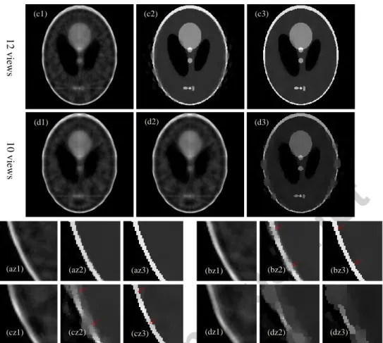
Fig. 3: Reconstructed images of the MLS phantom. (a1)-(a3), (b1)-(b3), (c1)-(c3) and (d1)-(d3) are the reconstructed images using the l2-norm regularization, TV regularization and the Gamma regularization with 18 views, 15 views, 12 views and 10 views, respectively.
(az1)-(az3), (bz1)-(bz3), (cz1)-(cz3) and (dz1)-(dz3) show the zoomed marked ROI in (a1)-(a3), (b1)-(b3), (c1)-(c3), and (d1)-(d3), respectively. l2-norm TV Gamma (c3) (c2) (d3) (d2) (d1)
(az1) (az2) (az3) (bz1) (bz2) (bz3)
(cz1) (cz2) (cz3) (dz1) (dz2) (dz3)
(a1) (a2) (a3)
(b3) (b2) (b1) (c1) 1 0 v iews 1 2 v iews 1 1 v iews 1 0 v iews
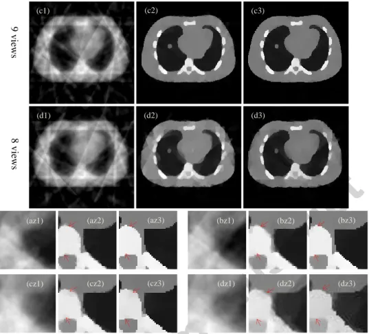
Fig. 4: Reconstructed images of the NACT phantom. (a1)-(a3), (b1)-(b3), (c1)-(c3) and (d1)-(d3) are the reconstructed images using the l2-norm regularization, TV regularization and the Gamma regularization with 11 views, 10 views, 9 views and 8 views,
respectively. (az1)-(az3), (bz1)-(bz3), (cz1)-(cz3) and (dz1)-(dz3) show the zoomed marked ROI in (a1)-(a3), (b1)-(b3), (c1)-(c3), and (d1)-(d3), respectively.
4.2. Visual evaluation of the simulation data.
Fig. 3 and Fig. 4 display the images reconstructed for performance assessment and comparison. For each phantom, a zoomed region of interest (ROI) is chosen (delineated by red line) to highlight the local image structures. The PSNR values of the reconstructed images are summarized in Tables 2 and 3. As it can be seen from (a1), (b1), (c1), (d1) and the zoomed ROI (az1), (bz1), (cz1), (dz1) in Fig. 3 and Fig. 4, the l2 -norm regularization fails to provide satisfying results in sparse-view reconstruction (some structures are blurred in the reconstruction). The reconstructions obtained with the Gamma and the TV regularizations lead to images with better visual quality than those resulting from the reconstruction based on the l2-norm regularization. When compared with the TV regularization, the proposed Gamma regularization provides a better contrast preservation (see the arrows in (bz3), (cz3) in Fig. 3 and the arrows in (az3)-(dz3) in Fig. 4). The performances of all the methods decrease as the number of projections decreases. The results of the TV regularization suffer from structure blurring and increased artifacts when the projection number is less than 12 for the MSL phantom and 10 for the NACT phantom (see the (az2), (bz2), (cz2), (dz2) in Fig. 3 and Fig. 4). However, even in these situations, the robustness of the proposed Gamma regularization appears much better as it is shown in the images (cz3) of Fig. 3 and Fig. 4).
4.3. Quantitative analysis of the simulation data. The PSNR values together with the corresponding
regularization parameters of the reconstructed images calculated via (9) are reported in Tables 2 and 3. These results confirm the observations made through visual image inspections. The PSNR values decrease
(c3) (c2) (c1) (d3) (d2) (d1)
(az1) (az2) (az3) (bz1) (bz2) (bz3)
(cz3) (cz2) (cz1) (dz1) (dz2) (dz3) 8 v iews 9 v iews
as the view number decreases and higher PSNR values are obtained for the Gamma regularization. Note that, for the two phantoms, α was set to 1.2 for the two phantoms and β according to the strategy described in section 3.2. [46].
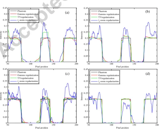
In Fig. 6 and Fig. 7, we plot the horizontal intensity profiles across the central lines of different reconstructed images (Fig. 5). Although the TV regularization performs already well, the Gamma reconstructions appear slightly better when matched to the ground truth phantom profiles.
Table 2: The PSNR (dB) of the reconstructed CT images with different view numbers for MSL phantom Phantom Methods 10 views 12 views 15 views 18 views
MSL l2-norm 22.67(λ=0.1) 24.10 (λ=0.1) 25.56 (λ=0.1) 26.07 (λ=0.1) TV 21.77 (λ=0.03) 25.28 (λ=0.03) 32.34 (λ=0.03) 38.67 (λ=0.05) Gamma (λ=0.1, α=1.2, β=8.55) (λ=0.1, α=1.2, β=7.59) (λ=0.1, α=1.2, β=6.67) (λ=0.1, α=1.2, β=5.83) 27.90 33.03 45.11 49.61
Table 3: The PSNR (dB) of the reconstructed CT images with different view numbers for NACT phantom Phantom Methods 8 views 9 views 10 views 11 views
NACT l2-norm 18.39 (λ=0.1) 19.05 (λ=0.1) 21.14(λ=0.1) 21.95 (λ=0.1) TV 23.73(λ=0.03) 28.68 (λ=0.03) 30.76 (λ=0.03) 34.16 (λ=0.03) Gamma (λ=0.01, α=1.2, β=9.07) (λ=0.1, α=1.2, β=10.85) (λ=0.01, α=1.2, β=9.65) (λ=0.01, α=1.2, β=8.78) 24.69 29.62 32.58 42.08
Fig. 5: The profiles (the 128th row from the top) of the two phantoms.
50 100 150 200 0 0.05 0.1 0.15 0.2 0.25 0.3 0.35 0.4 0.45 P ixel position In te n si ty P hantom Gamma regularization T V regularization l2-norm regularization 50 100 150 200 0 0.05 0.1 0.15 0.2 0.25 0.3 0.35 0.4 0.45 P ixel position In te n si ty P hantom Gamma regularization T V regularization l2-norm regularization 50 100 150 200 0 0.05 0.1 0.15 0.2 0.25 0.3 0.35 0.4 0.45 P ixel position In te n si ty P hantom Gamma regularization T V regularization l 2-norm regularization 50 100 150 200 0 0.05 0.1 0.15 0.2 0.25 0.3 0.35 0.4 0.45 P ixel position In te n si ty P hantom Gamma regularization T V regularization l2-norm regularization (a) (d) (c) (b) (a) (b)
Fig. 6: Intensity values along the horizontal profiles (the 128th row, as shown in Fig. 5 (a)) of the reconstructed MSL phantom images in Fig. 3. (a)-(d) are the horizontal profiles for the reconstruction with 10, 12, 15, 18 views, respectively.
Fig. 7: Intensity values along the horizontal profiles (the 128th row, as shown in Fig. 5 (b)) of the reconstructed NACT phantom images in Fig. 4. Note that (a)-(d) are the horizontal profiles for the reconstruction with 8, 9, 10, 11 views, respectively.
4.4. Experiments on clinical pelvis projection data
The proposed approach was also tested on a clinical pelvis projection data of a 56-year-old male patient
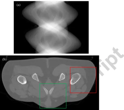
acquired on a monoenergetic Siemens Somatom CT system. The tube voltage and the current are 120 KVp and 100 mA, respectively. The image to reconstruct is composed of 256×256 pixels with 1mm×1mm pixel size. The imaging geometry is set as follows: the distance of source to center of rotation is 408 mm, and the distance of source to detector is 816 mm. A monochromatic single slice CT fan-beam scanner is imaged with a total of 360 scanning views and 512 radial bins per view. The acquired complete projection data is illustrated in Fig. 8 (a). For quantitative analysis purpose, a reference image (shown in Fig. 8 (b)) is reconstructed by means of a TV regularization using the complete projection data. Two ROIs (ROI1 and ROI2) marked in red and green rectangles are specified in Fig. 8 (b).
Fig. 9 to Fig. 12 illustrate the reconstruction results for l2-norm, TV, and Gamma regularizations with 1000 iterations for the uniformly-sampled 180, 120, 90 and 60 views, respectively. The regularization parameters λ, α and β are given in the corresponding figure captions below. We also display the two zoomed ROIs for comparison and we can observe much less strip artifacts in the reconstruction using Gamma regularization than other methods. Fig. 13 plots the PSNR values (with respect to the reference image in Fig. 8 (b)) for the whole image and two ROIs. We can see that the proposed method always leads to the highest PSNR among all the methods when the total sampling view is lower than 180.
Some ringing artifacts can be observed in Fig.4 (dz3) and Fig. 8-12 around the edge structures in the reconstructed images. As a matter of fact, the generated ringing artifacts are composed of the streak artifacts’ residues. The main reason is due to the regularization effects that are related to the combination of streak artifacts and the inherent image edges,which can be analyzed as follows. On the one hand, when compared to the l2-norm or TV regularization based algorithms, the proposed Gamma regularization significantly reduces streak artifacts in the homogeneous areas of the reconstructed images, whether it is the bright bone areas or the dark areas. On the other hand, in the high contrast connected areas, it cannot well distinguish the bright streak artifacts from bright bone areas as the l2-norm or TV regularization based
60 80 100 120 140 160 180 200 0 0.05 0.1 0.15 0.2 0.25 0.3 P ixel position In te n si ty P hantom Gamma regularization T V regularization l2-norm regularization 60 80 100 120 140 160 180 200 0 0.05 0.1 0.15 0.2 0.25 0.3 P ixel position In te n si ty P hantom Gamma regularization T V regularization l2-norm regularization 60 80 100 120 140 160 180 200 0 0.05 0.1 0.15 0.2 0.25 0.3 P ixel position In te n si ty P hantom Gamma regularization T V regularization l2-norm regularization 60 80 100 120 140 160 180 200 0 0.05 0.1 0.15 0.2 0.25 0.3 P ixel position In te n si ty P hantom Gamma regularization T V regularization l 2-norm regularization (a) (c) (d) (b)
algorithms. Thus, these streak artifacts’ residues are leaved around the bright bone areas and thus, ringing artifacts are formed. How to overcome this drawback, by means of postprocessing, such as segmentation, edge detection, etc., will be studied in our next work.
Fig. 8: (a) the complete pelvis projection data. (b) image reconstructed with TV regularization. Note that the two ROIs (ROI1 and ROI2) for more thorough analysis are delineated in red and green rectangles.
(a)
(b)
(a)
Fig. 9: Reconstructed pelvis CT images with 180 projections. (a)-(c): the images reconstructed by l2-norm regularization (λ=0.1), TV
regularization (λ=0.1), Gamma regularization (λ=1.8, α=1.2, β=2.4), respectively. (az1)-(cz1): the corresponding zoomed ROI1 in the (a)-(c). (az2)-(cz2): the corresponding zoomed ROI2 in the (a)-(c). (dz1) and (dz2) are the corresponding zoomed ROIs from the reference image in Fig. 8 (b).
(c) (cz1) (bz1) (az1) (cz2) (bz2) (az2) (a) (b) (dz1) (dz2)
Fig. 10: Reconstructed pelvis CT images with 120 projections. (a)-(c): the images reconstructed by l2-norm regularization (λ=0.1), TV
regularization (λ=1.3), Gamma regularization (λ=3, α=1.2, β=2.1), respectively. (az1)-(cz1): the corresponding zoomed ROI1 in the (a)-(c). (az2)-(cz2): the corresponding zoomed ROI2 in the (a)-(c). (dz1) and (dz2) are the corresponding zoomed ROIs from the reference image in Fig. 8 (b).
(c) (bz1) (az1) (cz1) (cz2) (bz2) (az2) (a) (b) (c) (dz1) (dz2)
Fig. 11: Reconstructed pelvis CT images with 90 projections. (a)-(c): the images reconstructed by l2-norm regularization (λ=0.1), TV
regularization (λ=1.3), Gamma regularization (λ=3.6, α=1.2, β=1.2), respectively. (az1)-(cz1): the corresponding zoomed ROI1 in the (a)-(c). (az2)-(cz2): the corresponding zoomed ROI2 in the (a)-(c). (dz1) and (dz2) are the corresponding zoomed ROIs from the reference image in Fig. 8 (b).
(a) (c) (b) (az1) (bz1) (cz1) (az2) (bz2) (cz2) (dz1) (dz2)
Fig. 12: Reconstructed pelvis CT images with 60 projections. (a)-(c): the images reconstructed by l2-norm regularization (λ=0.5), TV
regularization (λ=1.9), Gamma regularization ((λ=3.2, α=1.2, β=2.4), respectively. (az1)-(cz1): the corresponding zoomed ROI1 in the (a)-(c). (az2)-(cz2): the corresponding zoomed ROI2 in the (a)-(c). (dz1) and (dz2) are the corresponding zoomed ROIs from the reference image in Fig. 8 (b).
(az1) (bz1) (cz1) (cz2) (bz2) (az2) (dz1) (dz2) (a)
Fig. 13: PSNR of the reconstructed pelvis CT images using the different methods. (a): PSNR of the whole reconstructed images. (b): PSNR of the ROI1. (c): PSNR of the ROI2.
5. Discussion.
5.1. The RIP condition for the TV regularization
The RIP condition defined in [14, 58], is a key element in the CS theory. It is an important property of the sample matrix that evaluates the deviation between the reconstruction results and the optimal sparse approximation. This deviation for l1-norm regularization has been analyzed in [58].
Different from the canonical regularization term within the CS reconstruction model, TV regularization is used to constrain the total gradient fluctuations of the image to reconstruct. TV regularization has been widely employed in CS for image reconstruction [14]. Furthermore, the RIP condition of the sample matrix for the TV regularization has also been analyzed in [59] together with the sample condition in order to obtain satisfying reconstructions. More precisely, the relation between the RIP of the sample matrix and the reconstruction error has been established in [59]. When compared to the l1 -norm regularization, the total reconstruction error of TV regularization is not only up to the error between the gradients of the reconstruction results and the optimal sparse approximation, but also to the logarithmic value related to the pixel number in the target image [59].
5.2. Why the Gamma regularization works better than l1-norm?
The reason why the l0-norm regularization is better than the l1-norm in the case of highly limited measurements has been already theoretically proven in CS [14]. Therefore, because the Gamma regularization approaches closer to the l0-norm regularization than the l1-norm one in those points with larger gradients, it works better than l1-norm regularization in sparse-view reconstruction. This mechanism in modulating regularization effect is closely consistent with the intuitive observation that large gradients are often related to image edges while small gradients often come from noise and artifacts. A better preservation of edge structures with improved reconstruction quality can thus be achieved with the Gamma regularization.
5.3. Convergence analysis.
The first fidelity term in (5) is a function with strict convexity. However, a global minimum of the objection function cannot be guaranteed with Algorithm 1, as explained in the convexity analysis of the regularization term in the Appendix below.
Nevertheless, according to the Armijo-Goldstein based backtracking line search step length setting strategy applied in our CG algorithm [46, 55, 56], the following relation can be easily established:
(c) (b)
2 1 1 1 1 2 1 2 ( ) 1 2 ( ) k k v h k k k k v h k k Gf y f f f Gf y f f f (10) where k f denotes the thk
iterated image in reconstruction, and k1f denotes
(
k
1
)
th. It can be seen that a monotonic decrement in iteration can be obtained for Algorithm 1, which means that a local minimum can be reached. The convergence behavior of our algorithm is similar to the majorization-minimization (MM) algorithm investigated in [60]. As a consequence, with the condition of accepted error tolerance, a local minimization can be carried out in practice.
Fig. 14: The PSNR (a) and logarithmic cost function values (b) over iterations for MSL phantom with 15 views and NACT phantom with 10 views.
We analyzed the monotonic property of the overall cost function (5) in Algorithm 1 via the reconstructions of the MSL phantom with 15 views and the NACT phantom with 10 views. All the reconstruction parameters were set according to Table 1. The evolutions of the cost function values and the PSNR values over iterations are displayed in Fig. 14 (a) and Fig. 14 (b). We can observe monotonic decreases of the cost function values and monotonic increases of the PSNR over the whole 5000 iterations, and this shows that the proposed algorithm provides a stable solution for sparse-view reconstructions.
Fig. 15. The reconstruction images with different iterations in the experiments using the MSL phantom with 15 views and the NACT phantom with 10 views. (a1) reconstructed image with 5000 iterations for MSL phantom (λ=0.1), PSNR=45.11. (a2) reconstructed
image with 10000 iterations for MSL phantom (λ=0.1), PSNR=48.50. (b1) reconstructed image with 5000 iterations for NACT phantom (λ=0.01), PSNR=32.58. (b2) reconstructed image with 10000 iterations for NACT phantom (λ=0.01), PSNR=37.21.
To explore the impact of the iterations, we also conducted experiments with the MSL phantom with 15 views and the NACT phantom with 10 views. The iteration numbers are set to 5000 and 10000, respectively. The reconstructed images are shown in Fig.15. It can be seen that the reconstructed images are not impacted by the iterations.
5.4. Initial condition analysis
Although the Gamma norm is not convex, our algorithm always converges to an ensured local minimization. To examine the influence of the initialization (i.e. zero-valued initial image or FBP initial reconstruction), we analyzed the reconstructions of the MSL phantom with 12 views and the NACT phantom with 10 views. The reconstruction results are depicted in Fig. 16. The balance parameter λ was here selected to get the reconstruction with the highest PSNR value. We can see that nearly the same reconstructed images with same PSNR values can be obtained for these two different initial conditions. Therefore, the proposed reconstruction method does not appear sensitive to initial conditions.
5.5. Computation complexity analysis.
The proposed method needs about 9 minutes for the simulated data experiments (5000 iterations) and the clinical data experiments (1000 iterations) which is more time-consuming than the reconstruction using TV (about 2 minutes) and l2-norm (less than 1 minute) based regularizations. This is mainly due to the CDF calculation of Gamma regularization in the step size searching. Approximations of the CDF will be studied in our future work to speed up the computation efficiency.
Fig.16. The reconstruction images with different initial conditions for the experiment using the MSL phantom with 12 views and the NACT phantom with 10 views. (a1) reconstructed image using FBP initial condition for MSL phantom (λ=0.08), PSNR=33.03. (a2) reconstructed image using all zero initial condition for MSL phantom (λ=0.1), PSNR=33.03. (b1) reconstructed image using FBP initial condition for NACT phantom (λ=0.01), PSNR=32.58. (b2) reconstructed image using all zero initial condition for NACT phantom (λ=0.01), PSNR=32.58.
5.6. Comparison with Hu’ l0-norm regularization.
In [45], Hu et al. proposed an l0-norm based helical CT reconstruction method. The so-called l0-norm is in fact an approximate mathematical l0-norm obtained by introducing a potential function:
t, log(t 1)
(11)
where ρ is a positive parameter. We compared the performance of the proposed Gamma regularization with Hu’s l0-norm regularization in our sparse-view CT reconstruction method. The MSL phantom with 12 views and the NACT phantom with 10 views were used for validation. All the involved parameters in Hu’
our algorithm leads to reconstructed images with better edge preservation than Hu’s method for sparse-view CT reconstruction (see the arrows in the zoomed images in Fig.17).
Fig. 17. The reconstruction images with Hu’s method and the proposed method. (a1) Hu’ method, λ=0.5, PSNR=31.37; and (b1), Hu’ method, λ=0.3, PSNR=30.98, (a2) the proposed method, λ=0.1, PSNR=33.03, (b2), the proposed method, λ=0.01, PSNR=32.58.
6. Conclusion.
In this paper, the Gamma regularization proposed in [46] was employed for sparse-view CT reconstruction. This Gamma regularization provides a tunable strategy of fractional order norm to improve the reconstruction. The performance of the proposed approach wasassessed on simulated phantoms and real clinical data. In the simulations on the MSL phantom, we conducted the reconstructions using 10, 12, 15 and 18 views. For the NACT phantom, the sampled 8, 9, 10 and 11 sinogram views were used. In the clinical data experiments, 180, 120, 90, 60 views were used. Comparisons with the TV and l2-norm regularizations were also conducted. Although more clinical applications are still required, the present visual and quantitative evaluations confirmed the benefits brought by our approach and that its advantage becomes more prominent as the projection number decreases. However, some ring artifact residuals remain in the reconstructed images. They are due to regularization effects related to the combination of streak artifacts and the inherent image edges. Operations like edge detection, segmentation [61] or classification [62] should be incorporated to our model capable to deal with these problems.
Currently, all the parameters involved in our approach were chosen according to the strategy reported in [46] where the shape parameter α was fixed to 1.2, and the scale parameter β set according to the image distribution histogram issued from a preliminary FBP reconstruction. Our future work will develop adaptive strategies for setting these parameters in order to better use the intrinsic image data features, and doing so, we will explore the connection between Gamma regularization and factor regularization [61-63]. Furthermore, this proposed method will be tested in other image processing direction, like segmentation [64], classification [65], and advanced medical imaging modalities, such as MRI [66-68], et al.
Its applicability in clinical setting requires however a significant acceleration which will be achieved by means of parallel computation based on Graphics Processing Unit (GPU).
Appendix.
We analyze the concavity of the Gamma regularization function (5) by evaluating its second order derivative. We can see in (7) that the first derivative of Gamma regularization function includes four terms, all with the same structure. The second order derivative can be derived by calculating the derivative of the first term in (7):
1 2 2 1, , 1 2 2 1, , , 1, , i j i j f f i j i j i j i j i j f f e f f f
1 2 2 1, , 1 2 2 1, , 1 2 2 1, , 2 2 2 2 1, , , 1, 3 2 2 2 1, , , 1, 1 2 2 1, , 1 i j i j i j i j i j i j f f i j i j i j i j f f i j i j i j i j f f i j i j f f e f f e f f f f f f e
1 2 2 1, , 2 2 2 1, , 1 2 2 2 2 , 1, 1, , , 1, 2 1, , 1 i j i j f f i j i j i j i j i j i j i j i j i j i j f f e f f f f f f f f
1 2 2 1, , 2 2 2 1, , 1 2 2 2 , 1, 1 1, , 1 i j i j f f i j i j i j i j i j i j f f e f f f f
1 2 2 1, , 2 2 2 1, , 1 2 2 2 , 1, 1, , i j i j f f i j i j i j i j i j i j f f e f f f f (A1)Similarly, we can obtain (A2), (A3) and (A4) for the remaining three terms and thus, the overall second order derivative of the regularization term is:
1 2 2 , 1 , 1 2 2 , 1 , , , 1 , i j i j f f i j i j i j i j i j f f e f f f
1 2 2 , 1 , 1 2 2 2 2 2 2 , 1 , , , 1 , 1 , i j i j f f i j i j i j i j i j i j f f e f f f f (A2)
1 2 2 1, , 1 2 2 1, , , 1, , i j i j f f i j i j i j i j i j f f e f f f
1 2 2 1, , 1 2 2 2 2 2 2 1, , , 1, 1, , i j i j f f i j i j i j i j i j i j f f e f f f f
(A3)
1 2 2 , 1 , 1 2 2 , 1 , , , 1 , i j i j f f i j i j i j i j i j f f e f f f
1 2 2 , 1 , 1 2 2 2 2 2 2 , 1 , , , 1 , 1 , i j i j f f i j i j i j i j i j i j f f e f f f f
(A4)
1
2 2 1, , 2 , 1 2 2 2 2 2 2 1, , , 1, 1, , i j i j i j f f i j i j i j i j i j i j f f f f e f f f f
1
2 2 , 1 , 1 2 2 2 2 2 2 , 1 , , , 1 , 1 , i j i j f f i j i j i j i j i j i j f f e f f f f
1
2 2 1, , 1 2 2 2 2 2 2 1, , , 1, 1, , i j i j f f i j i j i j i j i j i j f f e f f f f
1
2 2 , 1 , 1 2 2 2 2 2 2 , 1 , , , 1 , 1 , i j i j f f i j i j i j i j i j i j f f e f f f f
(A5) From (A5), we can see that if fi1,jfi j, fi1,jfi j, fi j, 1fi j, fi j,1fi j, 0, we have
1 2 2 1 2 , 4 0 i j f e f (A6) Otherwise, if
fi1,jfi j,
2 fi1,jfi j,
2 fi j, 1fi j,
2 fi j, 1fi j,
2
0, we get
2 , 0 i j f f s.t.
1 2 s Min (A7)Here, S
fi1,jfi j,
2, fi1,jfi j,
2, fi j, 1fi j,
2, fi j,1fi j,
2
and Mins denotes the minimumamong the four values in S. In the same way, we can define Maxs as the maximum among the four values in S and get (A8):
2 , 0 i j f f s.t.
1 2 s Max (A8)From above we can see that (A8) cannot well hold to ensure the overall convexity of the cost function (5) because the Maxs value is determined by the unpredictable intensity variation in the reconstructed images.
So, the global minimum cannot be obtained through Algorithm 1, and a local minimum solution can only be attained.
Acknowledgements
This research was supported by National Basic Research Program of China under grant (2010CB732503),
Natural Science Foundation under grants (81370040, 31100713), and the Open Fund of China-USA Computer Science Research Center (KJR16026) and by the Qing Lan Project of Jiangsu Province.
References
1. D. J. Brenner, C. D. Elliston, E. J. Hall and W. E. Berdon, “Estimated risks of radiation-induced fatal cancer from pediatric CT,” American journal of roentgenology, 2001, vol. 176, no. 2, pp. 289-296, 2001.
2. D. J. Brenner & E. J. Hall, “Computed tomography—an increasing source of radiation exposure,” New England Journal of Medicine, vol. 357, no. 22, pp. 2277-2284, 2007.
3. De González, A. B. & Darby, S, “Risk of cancer from diagnostic X-rays: estimates for the UK and 14 other countries”, The lancet, vol. 363, no. 9406, pp. 345-351, 2004.
4. J. Hsieh, “Computed Tomography Principles, Design, Artifacts, and Recent Advances”, Wiley, 2009.
5. J. Hsieh, “Adaptive streak artifact reduction in computed tomography resulting from excessive X-ray photon noise,” Medical Physics, vol. 25, no.11, pp. 2139-2147, 1998.
6. M. Kachelriess, O. Watzke, and W. A. Kalender, “Generalized multidimensional adaptive filtering for conventional and spiral single-slice multi-slice, and cone-beam CT”, Medical physics, vol. 28, no. 4, pp. 475-490, 2001.
7. G. L. Zeng, “A filtered back projection MAP algorithm with non-uniform sampling and noise modeling”, Medical physics, vol. 39, no. 4, pp. 2170-2178, 2012.
8. J. Wang, T. Li, H. Lu and Z. Liang, “Penalized weighted least-squares approach to sinogram noise reduction and image reconstruction for low-dose x-ray CT”, IEEE Transactions on Medical Imaging, vol. 25, no. 10, pp. 1272-1283, 2006.
9. Y. Chen, Q. Feng, L. M. Luo, P. Shi and W. Chen, “Nonlocal prior Bayesian tomographic reconstruction”, Journal of Mathematical Imaging and Vision, vol. 30, no. 2, pp. 133-146, 2008.
10. Y. Chen, Z. Yang, Y. N. Hu, G.Y. Yang, Y.C. Zhu, Y.S. Li, L. M. Luo, W. F. Chen and C. Toumoulin, “Thoracic low-dose CT image processing using an artifact suppressed large-scale nonlocal means,” Physics in medicine and biology, vol. 57, no. 9, pp. 2667-2668, 2012.
11. Y. Chen, X. D. Yin, L. Y. Shi, H. Z. Shu, L.M. Luo, J. L. Coatrieux and C. Toumoulin, “Improving abdomen tumor low-dose CT images using a fast dictionary learning based processing,” Physics in medicine and biology, vol. 58, no. 16, pp. 5803-5820, 2013.
12. Y. Chen, L. Y. Shi, Q. J. Feng, J. Yang, H. Z. Shu, L. M. Luo, J. L. Coatrieux and W. F. Chen, “Artifact suppressed dictionary learning for low dose CT image processing”, IEEE Transactions on Medical Imaging, vol. 33, no.12, pp. 2271-2292, 2014. 13. R. Gordon, R. Bender, G. T. Herman, “Algebraic reconstruction techniques for three-dimensional electron microscopy and
photography”, Journal of theoretical Biology, vol. 29, no. 3, pp, 471-48, 1970.
14. E. Candes, J. Romberg, and T. Tao, “Robust uncertainty principles: Exact signal reconstruction from highly incomplete frequency information”, IEEE Transactions on Information Theory, vol. 52, no. 2, pp. 489-509, 2006.
15. Z. Dong, P. Phillips, S. Wang, and J. Yang, “Exponential Wavelet Iterative Shrinkage Thresholding Algorithm for Compressed Sensing Magnetic Resonance Imaging”, vol. 322, pp. 115-132, 2015
16. D. Donoho, “Compressed sensing,” IEEE Transactions on Information Theory, vol. 52, no. 4, pp. 1289-1306, 2006.
17. Y. Zhang, G. Ji, and Z. Dong, “Exponential Wavelet Iterative Shrinkage Thresholding Algorithm with Random Shift for Compressed Sensing Magnetic Resonance Imaging”, IEEJ Transactions on Electrical and Electronic Engineering, vol. 10, no. 1, pp. 116-117
18. Y. Liu, J. Hu. “A neural network for ℓ1− ℓ2 minimization based on scaled gradient projection: Application to compressed sensing”, Neurocomputing, vol. 173, pp. 988-993, 2016.
19. Z. Wang, H. Li, Q. Zhang, et al. “Magnetic Resonance Fingerprinting with compressed sensing and distance metric learning”, Neurocomputing, vol. 174, pp. 560-570, 2016.
20. H. Lee, A. Battle, R. Raina, A. Y. Ng, “Efficient sparse coding algorithms”, In Advances in neural information processing systems, pp. 801-808, 2006.
21. Y. Deng, Y. Kong, F. Bao, Q. Dai, “Sparse Coding Inspired Optimal Trading System for HFT Industry,” IEEE Transactions on Industrial Informatics. vol. 11, no. 2, pp. 467-475, 2015.
22. Y. Zhu, S. Lucey, “Convolutional sparse coding for trajectory reconstruction”, IEEE Transactions on Pattern Analysis and Machine Intelligence, vol. 37, no. 3, pp. 529-540, 2015.
23. J. A. Tropp, A. C. Gilbert, M. J. Strauss, “Algorithms for simultaneous sparse approximation, Part I: Greedy pursuit”, Signal Processing, vol. 86, no. 3, pp. 572-588, 2006.
24. S. I. Lee, H. Lee, P. Abbeel, A. Y. Ng, “Efficient L1 regularized logistic regression”, In Proceedings of the National Conference on Artificial Intelligence, vol. 21, no. 1, pp. 401-408,2006.
25. J. Maiora, B. Ayerdi, M, Graña. Random forest active learning for AAA thrombus segmentation in computed tomography angiography images”, Neurocomputing, vol. 126, pp. 71-77, 2014.
26. Y. Kong, Y. Deng, Q. Dai. “Discriminative Clustering and Feature Selection for Brain MRI Segmentation”, IEEE Signal Processing Letters, vol. 22, no. 5, pp. 573-577, 2015.
27. M. Elad, M. Aharon. “Image denoising via sparse and redundant representations over learned dictionaries”, IEEE Transactions on Image Processing, vol. 15, no.12, pp. 3736-3745, 2006.
28. Y. Shen, J. Li, Z. Zhu, et al. “Image reconstruction algorithm from compressed sensing measurements by dictionary learning”, Neurocomputing, vol. 151: pp.1153-1162, 2015.
29. M. Lustig, D. Donoho, and J. M. Pauly, “Sparse MRI: The application of compressed sensing for rapid MR imaging. Magnetic Resonance in Medicine”, Magnetic resonance in medicine, vol. 58, no. 6, pp. 1182-1195, 2007.
30. J. Trzasko, A. Manduca, and E. Borisch, “Highly undersampled magnetic resonance image reconstruction via homotopic ell-0-minimization”, IEEE Transactions on Medical imaging, vol. 28, no. 1, pp. 106-121, 2009.
31. Y. J. Lu, X. Q. Zhang, A. Douraghy, D. Stout, J. Tian, T. F. Chan and A. F. Chatziioannou, “Source Reconstruction for Spectrally-resolved Bioluminescence Tomography with Sparse A priori Information”, Optics express, vol. 17, no. 10, pp. 8062-8080, 2009.
32. L. Y. Fang, S. T. Li, R. P. McNabb, Q. Nie, A. N. Kuo, C. A. Toth, J. A. Izatt and S. Farsiu, “Fast Acquisition and Reconstruction of Optical Coherence Tomography Images via Sparse Representation”, IEEE Transactions on Medical Imaging, vol. 32, no. 11, pp. 2034-2049, 2013.
33. L. I. Rudin, S. Osher and E. Fatemi, “Nonlinear total variation based noise removal algorithms”, Physica D: Nonlinear Phenomena, vol. 60, no. 1, pp. 259-268, 1992.
34. H. Y. Yu, G. Wang, “A soft-threshold filtering approach for reconstruction from a limited number of projections”, Physics in medicine and biology, vol. 55, no. 13, pp. 3905-3916, 2010.
35. E. Y. Sidky, C. M. Kao, and X. Pan, “Accurate image reconstruction from few-views and limited-angle data in divergent-beam CT,” Journal of X-Ray Science and Technology, vol. 14, no. 2, pp. 119-139, 2006.
36. G. H. Chen, J. Tang, S. Leng, “Prior image constrained compressed sensing (PICCS): A method to accurately reconstruction dynamic CT image from highly undersampled projection data sets”, Medical physics, vol. 35, no. 2, pp. 660-663, 2008. 37. P. T. Lauzier, J. Tang, G. H. Chen, “Prior image constrained compressed sensing: implementation and performance evaluation”,
Medical physics, vol. 39, no. 1, pp. 66-80, 2012.
38. Y. Lu, J. Zhao and G. Wang, “Few-view image reconstruction with dual dictionary”, Physics in medicine and biology, vol. 57, no. 1, pp.173-189, 2012.
39. H. Y. Yu and G. Wang, “Compressed sensing based interior tomography”, Physics in medicine and biology, vol. 54, no. 9 pp. 2791-2805, 2009.
40. Y. Liu, Z. R. Liang, J. H. Ma, et al., “Total Variation-Stokes Sparse-View X-ray CT Image Reconstruction, IEEE Trans. Med. Imaging”, IEEE Transactions on Medical Imaging, vol. 33, no. 3, pp. 749-763, 2014.
41. L. Liu, Lin W, Pan J, et al. “X-ray computed tomography using sparsity based regularization”, Neurocomputing, vol. 173, pp. 256-269, 2016.
42. W. H. Guo, W. T. Yin, “EdgeCS: Edge Guided Compressive Sensing Reconstruction”, in “Proceedings of SPIE Visual Communication and Image Processing”, pp. 77440L-1-77440L-10, 2010.
43. W. H. Guo and W. T. Yin, “Edge guided reconstruction for compressive imaging”, SIAM Journal on Imaging Sciences, vol. 5, no. 3, pp. 809-834, 2012.
44. O. Lee, J. M. Kim, Y. Bresler, and J. C. Ye, “Compressive Diffuse Optical Tomography: Non-Iterative Exact Reconstruction using Joint Sparsity”, IEEE Transactions on Medical Imaging, vol. 30, no. 5, pp. 1129-1142, 2011,
45. Y. Hu, L. Xie, L. Luo, L., J. C. Nunes and C. Toumoulin, “L0 constrained sparse reconstruction for multi-slice helical CT reconstruction”, Physics in medicine and biology, vol. 56, no. 4, pp. 1173-1189, 2011.
46. J. F. Zhang, Y. Chen, et al, “Gamma regularization based reconstruction for low dose CT”, Physics in medicine and biology, vol. 60, no. 17, pp. 6901-6921, 2015.
47. T. M. Peters, “Algorithms for fast back-and re-projection in computed tomography”, IEEE Transactions on Nuclear Science, vol. 28, no. 4, pp. 3641-3647, 1981.
48. W. Zhuang, S. S. Gopal, T. J. Hebert, “Numerical evaluation of methods for computing tomographic projections”, IEEE Transactions on Nuclear Science, vol. 41, no. 4, pp. 1660-1665, 1994.
49. P. M. Joseph, “An improved algorithm for reprojecting rays through pixel images,” Medical Imaging, IEEE Transactions on, vol. 1, no. 3, pp. 192-196, 1982.
50. R. Siddon, “Fast calculation of the exact radiological path of a three-dimensional CT array”, Medical physics, vol. 12, no. 2, pp. 252-255, 1985.
51. B. D. Man and S. Basu, “Distance-driven projection and backprojection in three dimensions”, Physics in medicine and biology, vol. 49, no. 11, pp. 2463, 2004.
52. R. V. Hogg J. W. Mckean and A. T. Craig, “Introduction to Mathematical Statistics”, Pearson, 2013. 53. S. Boyd, L. Vandenberghe, “Convex Optimization”, Cambridge University Press, 2004.
54. R. Fletcher and C. Reeves, “Function minimization by conjugate gradients”, The computer journal, vol. 7, no. 2, pp. 149-154, 1964.
55. M. Frank and P. Wolfe, “An algorithm for quadratic programming”, Naval research logistics quarterly, vol. 3, no. (1-2), pp. 95-110, 1956.