On the root mean square quantitative chirality and quantitative symmetry measures

HAL Id: hal-02122820

https://hal.archives-ouvertes.fr/hal-02122820

Submitted on 7 May 2019

HAL is a multi-disciplinary open access

archive for the deposit and dissemination of

sci-entific research documents, whether they are

pub-lished or not. The documents may come from

teaching and research institutions in France or

abroad, or from public or private research centers.

L’archive ouverte pluridisciplinaire HAL, est

destinée au dépôt et à la diffusion de documents

scientifiques de niveau recherche, publiés ou non,

émanant des établissements d’enseignement et de

recherche français ou étrangers, des laboratoires

publics ou privés.

Copyright

On the root mean square quantitative chirality and

quantitative symmetry measures

Michel Petitjean

To cite this version:

Michel Petitjean. On the root mean square quantitative chirality and quantitative symmetry measures.

Journal of Mathematical Physics, American Institute of Physics (AIP), 1999, 40 (9), pp.4587-4595.

�10.1063/1.532988�. �hal-02122820�

On the root mean square quantitative chirality

and quantitative symmetry measures

Michel Petitjeana)

ITODYS (CNRS, ESA 7086), 1 rue Guy de la Brosse, 75005 Paris, France 共Received 22 February 1999; accepted for publication 22 March 1999兲

The properties of the root mean square chiral index of a d-dimensional set of n points, previously investigated for planar sets, are examined for spatial sets. The properties of the root mean squares direct symmetry index, defined as the normal-ized minimnormal-ized sum of the n squared distances between the vertices of the d-set and the permuted d-set, are compared to the properties of the chiral index. Some most dissymetric figures are analytically computed. They differ from the most chiral figures, but the most dissymetric 3-tuples and the most chiral 3-tuples have a common remarkable geometric property: the squared lengths of the sides are each equal to three times a squared distance vertex to the mean point. © 1999

Ameri-can Institute of Physics.关S0022-2488共99兲01009-9兴

I. INTRODUCTION

Chirality and symmetry properties of a solid body can be viewed as a continuous varying quantity taking values over关0;1兴 rather than a logical property, i.e., the body is or is not symmetric or chiral. The use of a chirality measure seems to be introduced by Rassat.1Then, various quan-titative chirality or symmetry measures have been used.2–12This concept has received applications in physics, proposed mostly by the Avnir group.2–4

The root mean square chiral index CHI of a d-dimensional set of n points was defined12as the sum of the n squared distances between the vertices of the set and those of its inverted image, normalized to 4T/d, T being the inertia of the set. This index is computed after minimization of the sum of the squared distances in respect to all rotations and translations and all permutations between equivalent vertices. It was shown to be a second kind of continuous chirality measure taking values over 关0;1兴, the zero value corresponding to an achiral compound perfectly super-posed to its inverted image. Similarly, the direct symmetry index DSI of a d-dimensional set of n points is defined here as follows. When all vertices are unequivalent, DSI is undefined. When there are at least two equivalent vertices, the sum of the n squared distances between the vertices and those of the permuted set is minimized for all rotations and translations and permutations 共exclud-ing the identity permutation兲 between equivalent vertices. DSI is the ratio of this minimized sum to twice the inertia T of the set.

The quantitative symmetry and chirality concepts used here are fully different from those of Avnir et al. for the following reasons: no achiral reference is needed to compute CHI, no sym-metry assumptions are needed to compute CHI and DSI, no folding and unfolding process5 are needed here, the normalization are different, and the farthest point from the centroid is not needed here, and, of course, the extremal figures are different.

The properties of CHI were examined for monodimensional sets and planar sets.12 They are now examined for spatial sets. Hyperspatial sets共i.e., d is any positive integer兲 are examined when all vertices are unequivalent. The major difference between planar, spatial, and hyperspatial sets lies in the expression of the optimal rotation. The properties of DSI are also examined. For clarity, a set of n⫽3 points will be called a triangle. The most dissymetric triangles, i.e., those maximiz-ing DSI, are here analytically computed when there are two or three equivalent vertices.

a兲_{Phone: 33共0兲1 4427 4857; fax: 33 共0兲1 4427 6814; electronic mail: Petitjean@itodys.jussieu.fr}

4587

II. NOTATIONS

The notations are those used in Ref. 12. X0 and X1 are the n rows and d columns arrays of coordinates. X0 is the fixed set and X1 is to move. The quote denotes the transposition operator. All vectors are written as one-column matrices.

具

x兩y

典

is the scalar product of the vectors x and y, and when d⫽3, x∧y is their cross product. The trace and the determinant operators are denoted,

respectively, Tr and Det. Y1 is the rotated and translated image of X1, and D2⫽Tr„(X0⫺Y1)

•(X0⫺Y1…

⬘

) is the sum of the squared distances. D2 is minimized for rotation plus translation when X0 and X1 are centered before computing the optimal rotation. Translations will be no longer considered, and the centering condition will not be assumed unless otherwise mentioned. The following matrices are used: V00⫽X0

⬘

•X0, V11⫽X1

⬘

•X1, V10⫽X1

⬘

•X0, V01⫽V10

⬘

, and

T⫽(T0⫹T1)/2, T0⫽Tr共V00兲 and T1⫽Tr共V11兲 being the respective inertia of X0 and X1,

reduc-ing to the usual inertia when the arrays are centered. The identity matrix is I, and R is a rotation matrix, such that Y1⫽X1•R

⬘

.

The correspondence between X0 and X1 is handled via an n-dimensional square permutation matrix P. Let be Z1⫽P•Y1. When X1 is the inverted image of X0 and when the centering condition is satisfied, the chiral index of a spatial set is CHI⫽D2/(4T/d), with D2⫽Tr„(X0

⫺P•X1•R

⬘

)•(X0⫺P•X1•R

⬘

)

⬘

… being minimized over all rotations R and allowed permutations

P. When X1 is a rotated and translated image of X0 and when the centering condition is satisfied,

DSI⫽D2/2T, D being minimized over all rotations and allowed nonidentity permutations. The computation of either CHI or DSI requires the optimal rotation superimposing two sets. When d⫽3, the analytical expression of the optimal rotation superposing X1 on X0, X0 and X1 being any n rows and 3 columns arrays of coordinates, is given in the Appendix.

III. THE OPTIMAL ROTATION FOR 3D ENANTIOMERS

In this section, the centering condition is not assumed and three-dimensional enantiomers are considered. For clarity, X0 is noted ⬃X and its inverted image is X1⫽⫺P•X, and we define

V⫽X

⬘

•P•X⫽⫺V01. From Appendix A, we have

D2⫽D02⫺2

具

q兩Bq

典

, 共1兲 the optimal quaternion q being the eigenvector associated to L1, the highest eigenvalue of B:

B⫽

冉

0 c

⬘

c A

冊

, 共2兲 A⫽Tr共V⫹V

⬘

兲•I⫺共V⫹V

⬘

兲, 共3兲 c⫽

冉

V共2,3兲⫺V共3,2兲 V共3,1兲⫺V共1,3兲 V共1,2兲⫺V共2,1兲

冊

. 共4兲

When P is a symmetric permutation, c is null, and the eigenvalues of B are the three eigenvalues of A and zero.

IV. ENANTIOMERS WITH ALL VERTICES UNEQUIVALENT

All the conditions of the preceding section are assumed to stand, and the vertices are all unequivalent, i.e., the only allowed permutation is P⫽I. V⫽X

⬘

•X is symmetric and c is therefore null. The sum of squares prior rotation is D02⫽4 Tr(V), which is the maximized D2 value because zero is the smallest eigenvalue of B. We have A⫽2„Tr(V)•I⫺V…. Let v1, v2, v3 be the eigenvalues of V arranged in decreasing order. The largest eigenvalue of B is L1⫽d1⫽2共v1⫹v2兲 and the optimal rotation of⫺X is 180 degrees around the principal axis associated to the smallest eigenvalue of V. Now we have D2⫽4 Tr(V)⫺4(v1⫹v2), i.e.,

D2⫽4v3. 共5兲

We assume now that X is centered, i.e., V is n times its variance matrix. The chiral index of the set of n vertices is therefore:

CHI⫽3v3/共v1⫹v2⫹v3兲. 共6兲

CHI is d times the percentage of inertia associated to the smallest eigenvalue of V. Looking at Eqs.共3兲 and 共7兲 in Ref. 12 and Appendix 1 in Ref. 12, we can see that this is also true for planar sets (d⫽2) and unidimensional sets (d⫽1).

The eigenvalues of V being positive and in decreasing order, CHI is maximized for v1⫽v2⫽v3⫽v, i.e., CHI⫽1 and V⫽v•I. When X has only 4 vertices, it is therefore a regular tetrahedron共see Appendix 2 in Ref. 12兲.

V. HYPERSPATIAL SETS WITH ALL UNEQUIVALENT VERTICES

The optimal rotation superimposing two d-dimensional sets is unknown when d⬎3, except for enantiomers with all unequivalent vertices, as shown hereafter. The sum of squares to be mini-mized is D2⫽Tr„(X⫺X•Q

⬘

)•(X⫺X•Q

⬘

)

⬘

…⫽2„Tr(X

⬘

•X)⫺Tr(Q•X

⬘

•X)…, X being the 共n,d兲 ar-ray of coordinates and Q being an orthogonal matrix with det(Q)⫽⫺1. Thus, Tr(Q•X

⬘

•X) has to be maximized. Assuming that X is in its principal components axis共i.e., V⫽X

⬘

•X is diagonal兲, we have to find the maximum of E⫽v共1兲•Q共1,1兲⫹v共2兲•Q共2,2兲⫹...⫹v(d)•Q(d,d),v共1兲,...,v(d) being the eigenvalues of V in decreasing order.

E⫽关„v共1兲⫺v共d兲…•Q共1,1兲⫹„v共2兲⫺v共d兲…•Q共2,2兲⫹¯⫹„v共d⫺1…⫺v共d兲兲

•Q共d⫺1,d⫺1兲兴⫹v共d兲•Tr共Q兲.

The eigenvalues of Q can be either⫹1, or ⫺1, or pairs of conjugate complex roots of 1. It follows that Tr(Q) is maximized when d⫺1 eigenvalues are ⫹1 and one is ⫺1. Obviously, the sum of the d⫺1 terms (v(i)⫺v(d)…•Q(i,i) is also maximized for Q(i,i)⫽1 when i⬍d. Thus E is maximized and D2 is minimized when X and its enantiomer have opposite coordinates on the principal axis with smallest inertia. Thus, Eqs.共5兲 and 共6兲 are generalized:

D2⫽4v共d兲, 共7兲

and assuming X centered:

CHI⫽d•v共d兲/„v共1兲⫹v共2兲⫹¯⫹v共d兲…. 共8兲

As previously, CHI is maximized when all eigenvalues of V are equal. When n⫽d⫹1, CHI is therefore maximized when X is a regular d-simplex.共See Appendix 2 in Ref. 12.兲

From Eq.共8兲, it is possible to compare practical CHI values with the distribution of CHI when

X is an isotropic multinormal sample. V is a Wishart matrix,13from which the joint density of the percentages of inertia can be derived,14 leading to the distribution15of CHI/d. Unfortunately, the final expression is not trivial when d⬎2.

VI. THE DIRECT SYMMETRY INDEX

In this section, d-dimensional sets are considered and the centering condition is not assumed. The situation where all vertices are unequivalent precludes the existence of direct symmetry in the set. This situation should not be confused with the purely geometric situation where all vertices are equivalent 共i.e., undistinct兲, for which symmetry properties are potentially observable. Thus, we consider now only sets with at least two equivalent vertices. As for the chiral index, the sum D2

of the n squared distances between the vertices and those of the permuted set is minimized for all rotations and all authorized permutations, excluding of course the identity permutation P⫽I. When the set is centered DSI⫽D2/(2T).

P being fixed, the sum of the squared distances to minimize is, as previously, D2⫽Tr„(X0

⫺P•X1•R

⬘

)•(X0⫺P•X1•R

⬘

)

⬘

…. Setting X0⫽X1⫽X and V⫽X

⬘

•P•X, we get

D2⫽2„T⫺Tr共V•R

⬘

兲…. 共9兲

There are at least two equivalent points x and y. Thus the minimum of D2for all rotations and permutations cannot exceed the minimum of D2for all rotations and for the permutation exchang-ing x and y, i.e., P is such that V⫽x•y

⬘

⫹y•x

⬘

⫹Z

⬘

•Z, with Z being the (n⫺2,d) block extracted from X by elimination of x and y. For this permutation,

Tr共V•R

⬘

兲⫽y

⬘

•R

⬘

•x⫹x

⬘

•R

⬘

•y⫹Tr共Z

⬘

•Z•R

⬘

兲. 共10兲

Assuming d⬎1, a rotation exists R which rotates from ⫹90 degrees the first axis toward the second axis, i.e., R(2,1)⫽⫺R(1,2)⫽1, R(i,i)⫽1 for i⬎2, all other elements of R being null. Thus, R⫹R

⬘

⫽0, y

⬘

•R

⬘

•x⫹x

⬘

•R

⬘

•y⫽0 and ⫺Tr(Z

⬘

•Z•R

⬘

)⫽Tr(Z

⬘

•Z•R)⫽Tr(R

⬘

•Z

⬘

•Z)

⫽Tr(Z

⬘

•Z•R

⬘

)⫽0, which means that Tr(V•R

⬘

) is null. Because a permutation and a rotation exist such that Tr(V•R

⬘

)⫽0, it follows from 共9兲 that the minimum of D2is upper bounded by 2T, and then DSI pertains to 关0;1兴 when d⬎1.

The following centered set containing three points is such that DSI⫽1 for all d⬎1: x⫽e1

•(⫺1⫺))/2, y⫽e1•(⫺1⫹))/2, z⫽e1, e1 being the first base vector, x and y being equivalent

and z being not.

When d⫽1, x and y are numbers, Z is a vector, T⫽x2⫹y2⫹Z

⬘

•Z, R⫽1, and Tr(V•R

⬘

)

⫽2x•y⫹Z

⬘

•Z. Thus, 4T⫺D2_{⫽2•„T⫹Tr(V•R}

_⬘

_{)…⫽2(x⫹y)}2_⫹4•Z

_⬘

_{•Z, which cannot be}

nega-tive. Thus, for d⫽1, D2 _{varies from 0 to 4T and the direct symmetry index pertains to关0;2兴, the}

extremal value DSI⫽2 being reached for a centered set containing two opposite values. But of course, direct rotational symmetry has little interest for d⫽1.

Computing simultaneously CHI and DSI for spatial sets is easy, since they both lead to the same quadratic form defined by Eqs.共1兲–共4兲, except that the quadratic form associated to DSI now takes the opposite sign, because X1 was set to X rather than to ⫺X. It means that the smallest eigenvalue L4 should be used to compute DSI rather than L1 for CHI, the minimized sum of squared distances being now

D2⫽D02⫹2L4. 共11兲

As shown in the Appendix, L4 is always nonpositive. Another difference between CHI and DSI is that the normalizing coefficients are, respectively, 4T/d and 2T, but this is not a crucial difference.

VII. THE DIRECT SYMMETRY INDEX OF PLANAR TRIANGLES

We assume that d⫽2. Let x be the column vector of the abscissas, and y the column vector of their ordinates: x

⬘

⫽(x1,x2,...,xn) and y

⬘

⫽(y1,y2,..., yn). The points will be p1, p2,..., pn. The image of共x,y兲 through the permutation P is 共Px,Py兲. P being fixed, the distance D minimized for all rotations is known:12

D2⫽2共T⫺E兲, 共12兲

E being the non-negative number, such that

E2⫽共x

⬘

P

⬘

x兲2⫹共x

⬘

P

⬘

y兲2⫹共y

⬘

P

⬘

x兲2⫹共y

⬘

P

⬘

y兲2⫹2共x

⬘

P

⬘

x兲共y

⬘

P

⬘

y兲⫺2共y

⬘

P

⬘

x兲共x

⬘

P

⬘

y兲.

Thus,

E2⫽共x

⬘

Px⫹y

⬘

P y兲2⫹共y

⬘

Px⫺x

⬘

P y兲2. 共13兲 The minimization for rotations plus translations is reached when the set is centered. The inertia is thus T⫽x

⬘

x⫹y

⬘

y . We assume T non-null, i.e., there are at least two distinct points. Let 1 be the n-vector such that all its n components are 1. Centering means 1

⬘

x⫽1

⬘

y⫽0. We define also M

⫽(P⫹P

⬘

)/2 and N⫽(P⫺P

⬘

)/2, which implies that x

⬘

Nx⫽y

⬘

Ny⫽0.

We assume now that n⫽3, and that all vertices are equivalents. d12, d23 and d31 are the

respective lengths of the sides of the triangle.储p1储, 储p2储 and 储p3储 are the lengths of the segments

joining the barycenter to the vertices at the opposite of the sides with respective lengths d23, d31

and d12. The inertia can be also written as T⫽储p1储2⫹储p2储2⫹储p3储2, or T⫽(d23 2_⫹d 31 2_⫹d 12 2 )/3. The surface S of the triangle is such that 16S2⫽2(d₁₂2 d₂₃2 ⫹d₂₃2 d2₃₁⫹d₃₁2 d₁₂2 )⫺(d₁₂4⫹d₂₃4

⫹d31 4

).

A. Extremal values for a given permutation

Using M and N, Eq.共13兲 becomes

E2⫽共x

⬘

M x⫹y

⬘

M y兲2⫹4共x

⬘

N y兲2. 共14兲 The gradient of (1⫺D2/2T)2⫽(E2/T2) if set to zero for x, then for y,

T共x

⬘

M x⫹y

⬘

M y兲Mx⫹2T共x

⬘

Ny兲Ny⫽E2x, 共15兲

T共x

⬘

M x⫹y

⬘

M y兲My⫺2T共x

⬘

N y兲Nx⫽E2y . 共16兲

Multiplying on the left共15兲 by x

⬘

then共16兲 by y

⬘

, and substracting,

T共x

⬘

M x兲2⫺T共y

⬘

M y兲2⫽E2共x

⬘

x⫺y

⬘

y兲. 共17兲

Then from共15兲 or 共16兲,

T共x

⬘

M x⫹y

⬘

M y兲共x

⬘

M y兲⫽E2共x

⬘

y兲 . 共18兲

From 共17兲 and 共18兲, it comes

E2共x

⬘

M y兲共x

⬘

x⫺y

⬘

y兲⫽E2共x

⬘

y兲共x

⬘

M x⫺y

⬘

M y兲. 共19兲

When n⫽3,5 permutations are possible: 3 are symmetric and 2 are circular.

When P is symmetric, M⫽P, N⫽0, and Eqs. 共15兲 and 共16兲 reduce to the same eigenvalues equations: T2_Px⫽E2_{x and T}2_Py⫽E2_{y . For n⫽3, the eigenvalues of P are ⫹1, ⫹1 and ⫺1. Only}

the solution such that E2_⫽T2_{is possible, implying D⫽0, leading to a minimum for DSI, rather to}

a maximum.

When P is one of the 2 circular permutations共the other being its transposed兲, we have: 2M

⫽1•1

⬘

⫺I, implying that x

⬘

M x⫽⫺x

⬘

x/2 and y

⬘

M y⫽⫺y

⬘

y /2, and then E2⫽4(x

⬘

N y )2⫹T2/4. Moreover, 2x

⬘

N y is equal to the determinant of the matrix 关1兩x兩y兴 or to the opposite of this

determinant, depending on which circular permutation is used. That implies E2⫽4S2⫹T2/4. The minimum is therefore reached by a null-area triangle: the points are aligned.

B. Maximizing DSI

Let us consider the symmetric permutation associating p1 to itself. The following comes: N

⫽0 and E2_⫽2x 2x3⫹x1 2_⫹2y 2y3⫹y1 2_⫽(T⫺d 23

2 ₎2_{. Similarly, the E values associated with the}

symmetric permutations associating p₂ with p₂ and p₃ with p₃ are such that E2⫽(T⫺d₃₁2)2 and

E2⫽(T⫺d12 2

)2. Both circular permutations lead to E2⫽4S2⫹T2/4, S2and T being homogeneous polynomials of d₁₂2, d₂₃2 and d₃₁2. The 4 expressions of E2 are homogeneous polynomials of 3 variables, returning non-negative values.

For a given triangle, the optimal permutation is that which leads to the highest E value. Thus a maximum of DSI, or a minimum of 关Max(E2)/T2兴, should be searched either among the extrema of E2/T2 associated with a permutation, or at the intersection of at least two of the 4 polynomials associated with the permutations, T being the same for all permutations.

It was shown above that only one extremum of E2/T2is useful, and it is such that E⫽T/2 and

S⫽0. This is possible only if the length of a side is equal to the sum of the two others. Assuming

for example, that d23⫽d31⫹d12, and reporting it in E⫽兩T⫺d23 2_兩⫽兩d 12 2_⫹d 31 2_⫺2d 23 2_{兩/3. The}

fol-lowing comes: E⫽(d₂₃2 ⫹2d₁₂d₃₁)/3, or E⫽(T/2)⫹d₁₂d₃₁. The circular permutation could be optimal only if d₁₂d₃₁⫽0, which should imply that DSI⫽0 共degenerate isocele triangle兲. Similar

conclusions should be reached if d31or d12have been used: the extrema of E2/T2 associated to a

given permutation are not adequate.

Thus, it is needed to look at the intersection of the polynomials. Noting that the E/T values depend only on the distances ratios, we can work with only two independent variables, and we search the minimum at the intersection of 3 among the 4 polynomials. There are at least 2 among 3 symmetric permutations which lead to the same value. Assuming, for example, that E⫽兩T

⫺d12 2_{兩⫽兩T⫺d} 31 2_{兩, thus, 兩d} 23 2 _⫹d 31 2 _⫺2d 12 2_兩⫽兩d 12 2 _⫹d 23 2 _⫺2d 31 2_{兩. Either we get d} 12 2_⫽d 31 2_{, which does}

not work because the triangle should be isocele (DSI⫽0), or we get 2d₂₃2⫽d₃₁2⫹d₁₂2, and thus

E⫽兩d12 2 _⫺d

31

2_{兩/2. In this situation, the E value associated to the third symmetric permutation is}

null, and the E value associated to circular permutations is E⫽d12d31. The equality between the

3 nonzero E2values give the desired relation: (d₁₂2 ⫺d₃₁2)2⫽4d₁₂2d₃₁2. Reusing 2d₂₃2⫽d₃₁2 ⫹d₁₂2 , the ratios of the squared lengths of the sides are deduced: (d₁₂2 /d₂₃2)⫽1⫹&/2, (d₃₁2 /d₂₃2)⫽1⫺&/2, and E2/T2⫽(1⫺DSI)2⫽1/2.

C. Remarkable geometric properties of the optimal triangles

Using the distances, we get the angles associated, respectively, to the points p1, p2 and

p3:␲/4, ␲/8 and 5␲/8.

A possible set of coordinates of the most dissymetric triangle is

X⫽

冉

&/3 1/3

共⫺3⫺&兲/6 ⫺1/6 共3⫺&兲/6 ⫺1/6

冊

. 共20兲

It is easy to see that d₂₃2 ⫽3储p1储2, d12 2_⫽3储p

2储2, and d31 2 _⫽3储p

3储2. It should be pointed out that

this relation is symmetric only for p2 and p3. This remarkable proportionality exists also for the

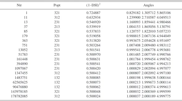
degenerate triangle with only two equivalent vertices, which was cited in Sec. VI, and correspond-ing to the maximal value DSI⫽1, for any dimension d⬎1. For d⫽2, the most chiral triangles also offer this remarkable proportionality, discarding which vertices are equivalent,12but none of them has the shape of the most dissymmetric triangle. The shape of the most dissymmetric triangle has been measured using random triangles, with vertices uniformly distributed over a square. The results共Table I兲 are in accordance with the theory.

VIII. DISCUSSION AND CONCLUSION

The properties of the RMS共root mean square兲 chiral index have been examined for spatial sets. As for planar sets, it is easily analytically computed, but the expression of the optimal 3D rotation is fully different from those of the 2D one. The optimal rotation is unknown for hyper-spatial sets, except when X is superposed with its unpermuted enantiomer. When d⬎3, it is proposed to extend the iterative procedure16 to compute the optimal rotation superposing two

d-dimensional sets, and to use it for permuted enantiomers. Similarly, computing the RMS direct

symmetry index is easy for 2D and 3D sets, but suffers from the same limitation than the chiral index when d⬎3.

Looking at Eq. 共8兲, it is clear that the RMS chiral index is also extendible to continuous distributions with all distinct points, provided that the variance exists. When there are subsets of 4592 J. Math. Phys., Vol. 40, No. 9, September 1999 Michel Petitjean

undistinct points, handling continuous sets is more difficult, because the set of authorized permu-tations must be redefined. This latter remark applies to the direct symmetry index. Thus, the extension of CHI and DSI to continuous sets will be examined in a further work.

The most chiral triangles and the most dissymmetric triangles offer the same remarkable geometric property. Its extension to higher-dimensional simplices is an open problem.

The chiral index and the direct symmetry index provides a coherent quantification of rota-tional symmetries carrying more information than a boolean value indicating the presence or absence of such symmetries. Although a perfect symmetry can be destroyed when a small pertur-bation is applied, the ability to quantify proper and improper rotational symmetries provides a robust tool to overcome this problem. As a by-product of computing CHI or DSI, the axe and angle associated to the optimal quaternion locate nonambiguously the symmetry element. When computing either CHI or DSI, if more than one permutation leads to small values of the indices, the set of optimal quaternions provides informations about the existence of more than one sym-metry element. Building an automated procedure returning all symsym-metry elements of a perturbated symmetric set is currently investigated.

ACKNOWLEDGMENT

The author thanks Professor D. Avnir for useful discussions and encouragement to publish this work.

APPENDIX: THE OPTIMAL ROTATION FOR SPATIAL SETS

In this section, the centering condition is not assumed, and d⫽3. X0 and X1 are any n rows and 3 columns arrays of coordinates. The identity permutation P⫽I is assumed, but the final result will be valid for any P with replacing X1 by P•X1. The well-known Procrustes algorithm16,17 used to find the optimal orthogonal transformation superposing two d-sets does not work for enantiomers, because it leads always to D⫽0 and the optimal orthogonal matrix has a negative determinant (Det⫽⫺1). Some iterative procedures are available,18,19but the final expression of the optimal rotation was found by Diamond,20leading to express D2 with a quadratic form of the

TABLE I. Measure of the shape of the most dissymmetric triangle with three equivalent vertices. Ntr: number of random triangles. Popt: optimal permutation. DSI: direct symmetry index. The 3 angles are expressed as multiples of␲/8.

Ntr Popt (1-DSI)2 Angles

1 321 0.724887 0.829182 1.305712 5.865106 11 312 0.632934 1.239900 2.710587 4.049513 13 231 0.546920 1.160093 1.859441 4.980466 37 213 0.539919 1.004153 1.865056 5.130791 85 321 0.537833 1.120757 1.822010 5.057233 179 321 0.519058 0.988815 2.067136 4.944049 363 321 0.513820 0.993675 2.054628 4.951697 751 231 0.503264 1.007408 2.009480 4.983112 13052 213 0.501541 0.999541 2.006778 4.993681 51783 231 0.500970 1.001485 2.007749 4.990766 161448 231 0.500631 1.001784 1.999454 4.998762 394890 231 0.500541 1.000720 2.005067 4.994213 1097067 231 0.500420 1.000829 2.002094 4.997077 1347455 312 0.500412 1.000807 2.002092 4.997100 1483751 132 0.500085 1.000198 1.999638 5.000164 62565625 132 0.500073 1.000213 1.999673 5.000114 90476880 132 0.500062 1.000012 2.000374 4.999613 143978185 321 0.500048 1.000032 2.000369 4.999599 178782085 312 0.500024 1.000037 2.000189 4.999775

quaternion associated to the rotation. This quadratic form is maximized by an orthonormal basis of four quaternions. For convenience, the expression of the optimal rotation is retrieved here follow-ing a different presentation.

A 3D-rotation R is associated to a 3D rotation axis u and to a rotation angle r. This is expressed with a quaternion q⫽(p,u), with p⫽cos(r/2) and 储u储⫽

具

u兩u

典

1/2⫽sin(r/2). Thus

具

q兩q

典

⫽1, and the image of a point x through R is21 Rx⫽(1⫺2

具

u兩u

典

)x⫹2

具

u兩x

典

u⫹2p(u∧x).

Because (⫺p,⫺u) is the same rotation than (p,u), p is always taken non-negative, i.e., r takes values from 0 to 180 degrees.

Let c be the sum of the n vectors x1i∧x0i. Thus, we have c(1)⫽V10共2,3兲⫺V10共3,2兲,

c(2)⫽V10共3,1兲⫺V10共1,3兲, and c(3)⫽V10共1,2兲⫺V10共2,1兲. The matrix A is defined as A

⫽共V10⫹V01兲⫺Tr共V10⫹V01兲•I. Let D02 _{be the initial sum of squares, prior to rotating X1.}

Now, we have the following equalities:

具

Rx1i兩x0i典⫽ (1⫺2

具

u兩u

典

)

具

x1i兩x0i典⫹ 2

具

u兩x1i典具u兩x0i典

⫹2p

具

u∧x1i兩x0i典⫽ (1⫺2

具

u兩u

典

)

具

x1i兩x0i典⫹

具

u兩(x1i•x0i

⬘

⫹x0i•x1i

⬘

)u

典

⫹2p

具

u兩x1i∧x0i典. V10 is the sum of the n matrices x1i•x0i

⬘

, and Tr(V10) is the sum of the n quantities

具

x1i兩x0i

典

. Thus we get D2⫽D02⫺2

具

u兩Au

典

⫺4p

具

u兩c

典

. Let us define the 4⫻4 matrix B:

B⫽

冉

0 c

⬘

c A

冊

,

q⫽(p,u) being the unknown quaternion; it follows that: D2⫽D02⫺2

具

q兩Bq

典

.

B is a constant symmetric matrix depending only on the input data, and the quadratic form

具

q兩Bq

典

has to be maximized, q being a unit vector. This problem has a well-known solution:17the stationary points are an othonormal basis eigenvectors of B, and the associated eigenvalues are the optimal values of the quadratic form. The sense of each eigenvector is known because p must be non-negative. It is unimportant to get ⫹u or ⫺u when p⫽0. Let L1, L2, L3, L4 be the eigen-values arranged in decreasing order.

B is the sum of two 4⫻4 symmetric matrices. One contains only A and zeros on the first row

and column. Let B1 be this matrix. The other contains only c

⬘

on the right of the first row and c on the bottom of the first column, zero as a first diagonal element, and nine zeros in the remaining 3⫻3 block. Let B2 be this one-rank matrix, of which the four eigenvalues are obviously 储c储 and zero with three as multiplicity. Let d1, d2, d3 be the eigenvalues of A arranged in decreasing order. Thus, the following inequalities stand:22 the eigenvalues of A separate those of

B:L1⭓d1⭓L2⭓d2⭓L3⭓d3⭓L4, and 兩Li–di

⬘

兩⭐储c储 for i⫽1,2,3,4, di

⬘

being the ith greatest value among共0,d1,d2,d3兲.

Two situations may arise. If d1 and d3 have not the same sign, the first set of inequalities means that L1 and L4 have not the same sign. If d1 and d3 have the same sign, let us look at the determinant of B expressed after diagonalization of A. The components of c become c共1兲, c共2兲, c共3兲, and det(B)⫽⫺c共1兲2•d2•d3⫺c共2兲2•d1•d3⫺c共3兲2•d1•d2. This determinant cannot be positive, thus again L1 and L4 cannot have the same sign.

Thus L1 is always non-negative and L4 is always non-positive. The rotation minimizing D2is those associated to the quaternion q1, such that D2⫽D02⫺2L1, and the rotation associated to q4 such that D2⫽D02⫺2L4 is that which maximizes D2. D2 has one saddle point associated to q2 and one associated to q3.

Some minor properties of the four optimal quaternions are obtained from their othonormality. Considering the first row of the equation Bq⫽Lq, it comes that D02⫺D2⫽2L⫽2

具

v兩c

典

, withv

⫽u/p. It shows than only a positive L value leads to D2_⬍D02_{. The three others equations may be}

rewritten: (A⫺

具

v兩n

典

I)v⫹n⫽0, but this is neither an eigenvector equation nor a linear system.

Two distinct directions ui and uj are generally not orthogonal: cos(ui,uj)⫽⫺pi•pj/„(1⫺pi2_)•(1

⫺p j2_)…1/2_{⫽⫺cot g(ri)•cot g(rj), ri and rj being the 2D-angles associated, respectively, to qi}

and qj.

1_{A. Rassat, ‘‘Un crite`re de classement des syste`mes chiraux de points a` partir de la distance au sens de Haussdorf,’’}

Compt. Rend. Acad. Sci. Paris 299, Se´r. II, 53–55共1984兲.

2_{Y. Pinto, P. W. Fowler, D. Mitchell, and D. Avnir, ‘‘Continuous chirality analysis of model Stone–Wales}

rearrange-ments in fullerenes,’’ J. Phys. Chem. B 102, 5776–5784共1998兲.

3

D. R. Kanis, J. S. Wong, T. J. Marks, M. A. Ratner, H. Zabrodsky, S. Keinan, and D. Avnir, ‘‘Continuous symmetry analysis of hyperpolarizabilities. Characterization of the second-order nonlinear optical response of distorted benzene,’’ J. Phys. Chem. 99, 11061–11066共1995兲.

4_{V. Buch, E. Gershgoren, H. Zabrodsky Hel-Or, and D. Avnir, ‘‘Symmetry loss as a criterion for cluster melting, with}

application to共D2兲13,’’ Chem. Phys. Lett. 247, 149–153 共1995兲.

5_{H. Zabrodsky and D. Avnir, ‘‘Continuous symmetry measures. 4. Chirality,’’ J. Am. Chem. Soc. 117, 462–473共1995兲.} 6_{G. Gilat and Y. Gordon, ‘‘Geometric properties of chiral bodies,’’ J. Math. Chem. 16, 37–48共1994兲.}

7_{J. Maruani, G. Gilat, and R. Veysseyre, ‘‘Chirality limits of convex bodies,’’ Compt. Rend. Acad. Sci. Paris 319, Se´r. II,}

1165–1172共1994兲.

8

N. Weinberg and K. Mislow, ‘‘Distance functions as generators of chirality measures,’’ J. Math. Chem. 14, 427–450 共1993兲.

9_{Z. Zimpel, ‘‘A geometrical approach to the degree of chirality and asymmetry,’’ J. Math. Chem. 14, 451–465共1993兲.} 10_{J. Maruani and P. G. Mezey, ‘‘From symmetry to syntopy: a fuzzy-set approach to quasi-symmetric systems,’’ J. Chim.}

Phys. 87, 1025–1047共1990兲.

11

M. Petitjean, ‘‘Calcul de chiralite´ quantitative par la me´thode des moindres carre´s,’’ Compt. Rend. Acad. Sci. Paris, Se´r. IIc 2, 25–28共1999兲.

12_{M. Petitjean, ‘‘About second kind continuous chirality measures. 1. Planar sets,’’ J. Math. Chem. 22, 185–201共1997兲.} 13_{M. S. Srivastava and C. G. Khatri, An Introduction to Multivariate Statistics共Elsevier, New York, 1979兲, Chap. 3.} 14

M. S. Bartlett, ‘‘The effect of standardization on a␹2 approximation in factor analysis,’’ Biometrika 38, 337–344 共1951兲.

15

F. J. Schuurmann, P. R. Krishnaiah, and A. K. Chattopadhyay, ‘‘On the distributions of the ratios of the extreme roots to the trace of the Wishart matrix,’’ J. Multivariate Anal. 3, 445–453共1973兲.

16_{J. R. Hurley and R. B. Cattell, ‘‘The Procrustes Program: Producing direct rotation to test a hypothesized factor}

structure,’’ Behav. Sci. 7, 258–262共1962兲.

17_{G. H. Golub and C. F. Van Loan, Matrix Computations共Johns Hopkins University Press, Baltimore, 1985兲, Secs. 8.1 and}

12.4.

18_{A. D. McLachlan, ‘‘Rapid comparison of protein structures,’’ Acta Crystallogr. Sect. A: Cryst. Phys., Diffr., Theor. Gen.}

Crystallogr. 38, 871–873共1982兲.

19_{M. J. Sippl and H. Stegbuchner, ‘‘Superposition of three-dimensional objects: A fast and numerically stable algorithm}

for the calculation of the matrix of optimal rotation,’’ Comput. Chem. 15, 73–78共1991兲.

20

R. Diamond, ‘‘A note on the rotational superposition problem,’’ Acta Crystallogr., Sect. A: Found. Crystallogr. 44, 211–216共1988兲.

21_{R. Deheuvels, Formes Quadratiques et Groupes Classiques共Presses Universitaires de France, Paris, 1981兲, p. 375.} 22_{J. H. Wilkinson, The Algebraic Eigenvalue Problem共Clarendon, Oxford, 1965兲, Secs. 39–41.}