READ THESE TERMS AND CONDITIONS CAREFULLY BEFORE USING THIS WEBSITE.
https://nrc-publications.canada.ca/eng/copyright
Vous avez des questions? Nous pouvons vous aider. Pour communiquer directement avec un auteur, consultez la première page de la revue dans laquelle son article a été publié afin de trouver ses coordonnées. Si vous n’arrivez Questions? Contact the NRC Publications Archive team at
[email protected]. If you wish to email the authors directly, please see the first page of the publication for their contact information.
NRC Publications Archive
Archives des publications du CNRC
Access and use of this website and the material on it are subject to the Terms and Conditions set forth at Data pooling and key comparison reference values
Steele, A.; Hill, K.
https://publications-cnrc.canada.ca/fra/droits
L’accès à ce site Web et l’utilisation de son contenu sont assujettis aux conditions présentées dans le site LISEZ CES CONDITIONS ATTENTIVEMENT AVANT D’UTILISER CE SITE WEB.
NRC Publications Record / Notice d'Archives des publications de CNRC: https://nrc-publications.canada.ca/eng/view/object/?id=e32d8a84-62d6-4f0f-84df-d7a5a8bb57f2 https://publications-cnrc.canada.ca/fra/voir/objet/?id=e32d8a84-62d6-4f0f-84df-d7a5a8bb57f2
Data Pooling and Key Comparison Reference Values
A.G. Steele and K.D. Hill National Research Council of Canada
As we are all aware, the usual practice for reporting Key Comparison data is to take a key comparison reference value (KCRV) as the baseline, since “it is required by the MRA”. In fact, the current policy for CIPM Key Comparisons conducted by the CCT requires a technical explanation in cases where a comparison is to be reported without a KCRV. In this short note, we contend that more careful consideration of the comparison data sets is required to justify the use of a KCRV, and that reliance on policy when arguing in favor of a KCRV is not always warranted for the particular data sets obtained experimentally. We consider explicitly the case for comparisons near the triple point of argon, performed in two different Key Comparisons, each using a very different experimental procedure.
There are several statistical calculations that are appropriate and useful for examining various candidate reference values, and for deciding whether or not the data is amenable to presentation in terms of a single KCRV. We can calculate the uniformly weighted mean, the mean weighted by the inverses of the experimental variances, and the median of the data set in an attempt to compare candidate quantities to be used as the KCRV. We can pool the data, combining the individual laboratory distributions, and obtain
information about the distribution we would expect to observe upon many repeats of the comparison. Similarly, we can calculate the distributions of the comparison mean, weighted mean, and median.
Much of this work can be done analytically, since the uncertainty budgets are generally expressed in terms of normal distributions. Calculating the distribution of the median is somewhat complicated, however, and is more easily accomplished using Monte Carlo techniques. We therefore use Monte Carlo simulations to predict each of the
aforementioned distributions, using 109 “rolls of the dice” to represent repeat comparisons, thus building up the statistical picture. For each “comparison” in the simulation, the laboratory data is obtained using a Gaussian random number generator, centred on the laboratory value and having a half-width equal to the laboratory
uncertainty. The pooled data distribution assumes that all laboratory data are
independent, and can thus be added directly. Each of the aggregate quantities (weighted mean, simple mean, and median) is calculated for each “comparison”, and a histogram is built up during the simulation to illustrate the corresponding distributions.
Consider the comparison data obtained near the triple point of argon from the report CCT-K2: Key Comparison of Capsule-type Standard Platinum Resistance Thermometers from 13.8 K to 273.16 K. In this experiment, each participant calibrated their
thermometers locally, and then carried the instruments to the Pilot laboratory for the comparison measurements. The experimental design of CCT-K2 was such that the “average temperature of the comparison block” was expected to be a physically meaningful quantity, since all of the thermometers in a given measurement sequence were loaded into the cryostat simultaneously, and the values indicated by each
thermometer were measured in round-robin fashion over a very short time interval. This might be the simplest comparison topology to imagine, where none of the artifacts were shipped during the measurement phase. The data near the argon point are summarized in Table 1.
Table 1. Comparison data near 83.8058 K for the Group B thermometers as presented in
the CCT-K2 Report. Lab (T – KCRV) / mK Uncertainty (k=1) / mK BNM-INM 0.11 0.22 IMGC -0.09 0.10 KRISS 0.01 0.17 NIST 0.04 0.11 NPL -0.04 0.13 NRC 0.24 0.22 PTB 0.22 0.21 Mean 0.07 Wt Mean 0.01 Median 0.04 -1.0 -0.8 -0.6 -0.4 -0.2 0.0 0.2 0.4 0.6 0.8 1.0 pooled data weighted mean simple mean median
Figure 1. Graphs of the CCT-K2 data near 83.8058 K. The expected distributions for i)
pooled laboratory data; ii) the weighted mean; iii) the simple mean; iv) the median, have been calculated using Monte Carlo techniques. This data set exhibits no obvious
The CCT-K2 data near 83.8058 K (shown in Figure 1) are pretty close to the ideal for a “successful” comparison: the data pool has an almost-normal distribution, and the simple mean, weighted mean, and median values are in reasonable agreement with each other. The pooled distribution is somewhat asymmetric, but not enough to “worry” us, or prevent the use of an aggregate statistical estimator to describe the comparison results.
The experiments in CCT-K2 represent the kind of comparison result that we believe the authors of the MRA had in mind when they proposed that all laboratory degrees of equivalence should be calculated through the degree of equivalence to the KCRV. There appears to be no compelling reason to reject the notion that a KCRV can be used as the baseline, and there is some scientific information available to assist in choosing among more-or-less equivalent candidate values.
In sharp contrast, consider a data set from the Report to the CCT on Key Comparison 3 (Comparison of Realization of the ITS-90 over the Range 83.8058 K to 933.473 K). CCT-K3 had a significantly more complicated experimental topology than that used for CCT-K2: a variety of fixed points and reference thermometers were circulated among the participants in three separate “loops” over a period of many months. Calculations were performed by the Pilot laboratory to account for substantially different correlation effects and degrees of freedom in the measurement results, and the final bilateral degrees of equivalence are summarized in an extensive set of tables and graphs.
Table 2 lists the laboratory values and comparison uncertainties for nine participants at the triple point of argon, 83.8058 K. We have chosen to display the results against the Pilot laboratory value in this presentation, although the Key Comparison report provides tables and graphs from all perspectives.
Table 2. Data from the CCT-K3 report at 83.8058 K.
Lab (T – TNIST) / mK Uncertainty (k=1) / mK
BNM -0.35 0.29 IMGC 0.73 0.26 NIM -0.24 0.33 NIST 0.00 0.04 NML -2.42 0.49 NPL -1.01 0.34 NRC 0.10 0.16 PTB -0.23 0.28 VSL -0.06 0.33 Mean -0.39 Wt Mean -0.02 Median -0.23
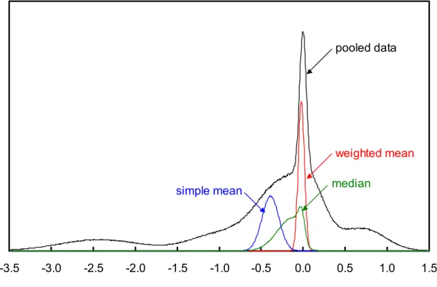
The Monte Carlo modeling for the pooled distribution and the distributions of the various “candidate KCRV” statistics is shown in Figure 2. In this particular example, the pooled
data distribution has at least four easily identifiable modes. The distributions for the mean and weighted mean appear to select two different modes. The median distribution is quite asymmetric, and almost bridges the gap between the uniformly weighted mean and the mean weighted by the inverses of the experimental variances: the mode of the median distribution is close to the weighted average of the pooled data (as seen in Figure 2), although the median itself is close to the simple average (as seen in Table 2).
All three of these candidate KCRV statistics are clearly unrepresentative of the underlying “population” of comparison data sets obtained by pooling the independent laboratory results. The pooled data is not normally distributed, and cannot be
unambiguously represented by a single measure of “central tendency”. In this case, the simple mean, the weighted mean, and the median should therefore be rejected as
aggregate estimators for use in summarizing this comparison in Appendix B of the MRA.
-3.5 -3.0 -2.5 -2.0 -1.5 -1.0 -0.5 0.0 0.5 1.0 1.5 pooled data
weighted mean
simple mean median
Figure 2. Graph of the CCT-K3 data at 83.8058 K. The expected distributions for i)
pooled laboratory data; ii) the weighted mean; iii) the simple mean; iv) the median have been calculated using simple Monte Carlo techniques.
In our experience, simple data pooling such as has been done in this paper can often provide insight into the appropriateness of statistical treatment of Key Comparison data. It is often the case that extremely careful and well-performed comparisons produce results which are not amenable to “blind statistical analysis”, and which should not be thought of in terms of a simple Key Comparison Reference Value.
Other questions, particularly the use of null hypothesis testing and the relevance of treating the widths of the aggregate statistical distributions as “uncertainties” for the corresponding candidate KCRV quantity, will be addressed in a more complete article.
For completeness, we have included the pooled distributions for all of the comparison values from the CCT-K2 and CCT-K3 reports as appendices to this brief report. Here, the distributions have been summed directly from the individual laboratory results without recourse to the Monte Carlo techniques mentioned previously.
Appendix 1. Pooled distributions based on the Group B data in the CCT-K2 report
For completeness, we include the pooled distributions for all of the Group B comparison values from CCT-K2. Here, the distributions have been summed directly from the individual laboratory results without recourse to the Monte Carlo techniques mentioned previously; the distributions for the mean, weighted mean, and median are not shown.
CCT-K2 eH2 Pooled Distribution -1.0 -0.5 0.0 0.5 1.0 ∆ ∆ ∆ ∆ T / mK CCT-K2 17K Pooled Distribution -1.0 -0.5 0.0 0.5 1.0 ∆ ∆ ∆ ∆ T / mK CCT-K2 20K Pooled Distribution -1.0 -0.5 0.0 0.5 1.0 ∆ ∆∆ ∆ T / mK CCT-K2 Ne Pooled Distribution -1.0 -0.5 0.0 0.5 1.0 ∆ ∆ ∆ ∆ T / mK
CCT-K2 O2 Pooled Distribution -1.0 -0.5 0.0 0.5 1.0 ∆ ∆ ∆ ∆ T / mK CCT-K2 Ar Pooled Distribution -1.0 -0.5 0.0 0.5 1.0 ∆ ∆ ∆ ∆ T / mK CCT-K2 Hg Pooled Distribution -1.0 -0.5 0.0 0.5 1.0 ∆ ∆∆ ∆ T / mK
Appendix 2. Pooled distributions based on the CCT-K3 report.
For completeness, we include the pooled distributions for all of the comparison values from the CCT-K3 report. Here, the distributions have been summed directly from the individual laboratory results without recourse to the Monte Carlo techniques mentioned previously; the distributions for the mean, weighted mean, and median are not shown.
CCT-K3 Ar Pooled Distribution -4 -2 0 2 4 ∆ ∆ ∆ ∆ T / mK CCT-K3 Hg Pooled Distribution -1.0 -0.5 0.0 0.5 1.0 ∆ ∆∆ ∆ T / mK CCT-K3 Ga Pooled Distribution -2 -1 0 1 2 ∆ ∆ ∆ ∆ T / mK CCT-K3 In Pooled Distribution -4 -2 0 2 4 ∆ ∆∆ ∆ T / mK
CCT-K3 Sn Pooled Distribution -4 -2 0 2 4 ∆ ∆ ∆ ∆ T / mK CCT-K3 Cd Pooled Distribution -4 -2 0 2 4 ∆ ∆∆ ∆ T / mK CCT-K3 Zn Pooled Distribution -4 -2 0 2 4 ∆ ∆ ∆ ∆ T / mK CCT-K3 Al Pooled Distribution -4 -2 0 2 4 ∆ ∆∆ ∆ T / mK