HAL Id: hal-00795078
https://hal.archives-ouvertes.fr/hal-00795078
Submitted on 27 Feb 2013
HAL is a multi-disciplinary open access
archive for the deposit and dissemination of sci-entific research documents, whether they are pub-lished or not. The documents may come from teaching and research institutions in France or abroad, or from public or private research centers.
L’archive ouverte pluridisciplinaire HAL, est destinée au dépôt et à la diffusion de documents scientifiques de niveau recherche, publiés ou non, émanant des établissements d’enseignement et de recherche français ou étrangers, des laboratoires publics ou privés.
M. Richier, R. Lenain, Benoît Thuilot, M. Berducat
To cite this version:
M. Richier, R. Lenain, Benoît Thuilot, M. Berducat. ATV rollover prevention system including varying grip conditions and bank angle. 3rd International Conference on Machine Control & Guidance, Mar 2012, Stuttgart, Germany. 10 p. �hal-00795078�
ATV rollover prevention system including varying grip
conditions and bank angle
Mathieu Richier1, Roland Lenain1, Benoit Thuilot2, 3, Michel Berducat 1 1
Cemagref, 24 avenue des Landais, 63172 Aubière, France
2
Clermont université, Université Blaise Pascal, Institut Pascal, BP 10448, 63000
Clermont-Ferrand, France
3
CNRS, UMR 6602, Institut Pascal, 63171 Aubière, France
Abstract
In this paper, an algorithm dedicated to light ATVs, which estimates and anticipates the rollover, is proposed. It is based on the on-line estimation of the Lateral Load Transfer (LLT), allowing the evaluation of dynamic instabilities. The LLT is computed thanks to a dynamical model split into two 2D projections. Relying on this representation and a low cost perception system, an observer is proposed to estimate on-line the terrain properties (grip conditions and slope), then allowing to deduce accurately the risk of instability. Associated to a predictive control algorithm, based on the extrapolation of rider’s action, the risk can be anticipated, enabling to warn the pilot and to consider the implementation of active actions.
Keywords
Light All-Terrain Vehicles (ATV), quad bikes, dynamic stability, Lateral Load Transfer (LLT), lateral rollover, sliding, modelling, observers and slope.
1 INTRODUCTION
Thanks to their high manoeuvrability, quad bikes are more and more popular and especially in agricultural context. Nevertheless, their mechanical properties lead to a significant rollover risk which constitutes the main cause of serious accidents for All-Terrain Vehicles (ATV) (almost 50 % of ATV crashes as mentioned in [1] and [2]). If a rollover protective structure (ROPS) may limit health damages, it is not convenient for light vehicles. In contrast, the development of active devices, improving the stability of ATVs, constitutes a promising solution.
In on-road context, some stability systems have been designed in order to improve vehicle stability such as [3], [4] and [5]. As they use a linear tire model, these algorithms are not adapted to large grip condition variations, encountered in off-road context.
Some systems dedicated to off-road mobile robots have been developed like [6], [7], [8] and [9]. However they are hardly transposable to light ATV, since the required sensors remain expensive such as highly accurate INS or RTK GPS. Moreover, the accessibility of GPS data cannot be ensured when the ATV moves in natural environment (trees, mountains, building, etc.).
In previous work [10], a rollover risk prevention system dedicated to high speed ATVs has been proposed, based on low cost sensing equipment. It estimates on-line the tire-ground friction. The Lateral Load Transfer (LLT) has been chosen as a relevant stability criterion among several rollover indicators [11], because low cost sensing equipment is sufficient to estimate it. The main limitation of this system was the assumption of a flat ground, which is not representative of off-road applications. A less important limitation was a singularity in the algorithm, which entails to stop grip conditions update. A new modelling and a new approach to the grip condition observation is proposed in this paper. With low cost sensing equipment composed of a 3-axes accelerometer/gyrometer, a Doppler radar and a steering angle sensor, the LLT can be predicted whatever the grip conditions and the slope. More precisely, a bicycle model is associated to an adapted backstepping observer, which estimates the sliding parameters and the slope. These estimations are then used within a prediction algorithm based on a roll model, in order to anticipate the LLT.
The paper is organized as follows: first, the vehicle modelling is depicted. It allows the rollover metric computation. As the LLT expression requires the knowledge of the sliding parameters, an adapted backstepping observer is developed in the second part. In the same part, a prediction algorithm allowing the anticipation of LLT time-evolution is described. Finally, full scale experiments (with a commercial quad bike) are presented to investigate the capabilities and the applicability of the proposed approach.
2 ROLLOVER METRIC COMPUTATION
2.1 Dynamic model
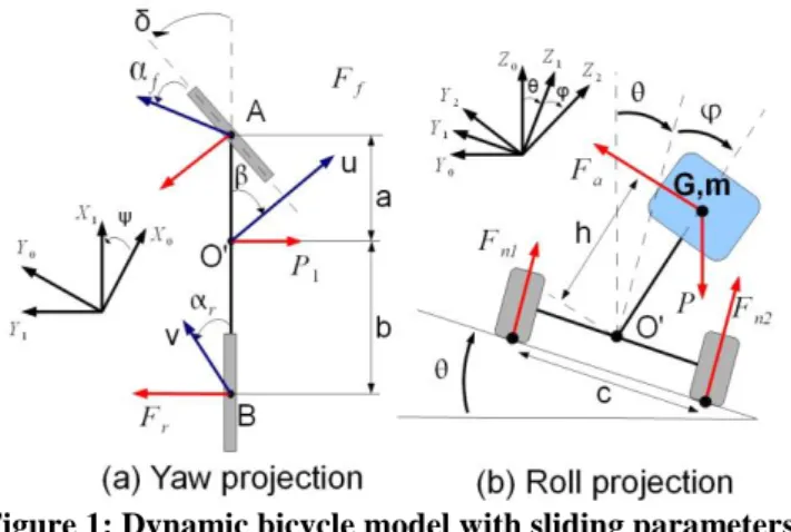
In order to achieve on-line LLT computation when the ground is uneven, the global vehicle modelling depicted on Fig.1 is considered. The dynamical model of vehicle is split into two models. The first model represents a yaw 2D projection (shown on Fig.1 (a)) assuming a flat ground. In order to account for ground variation, a lateral force (P1) is added. Relying on the state observer described in section 3, this model enables the estimation of the sliding parameters (sideslip angles , f, r and lateral forces
Ff and Fr) and the bank angle (θ), which significantly impact the risk of rollover. These sliding conditions are then injected into the second model: a roll 2D projection (shown on Fig.1 (b)) used to estimate the LLT.
Figure 1: Dynamic bicycle model with sliding parameters.
The variables and parameters used in the sequel, reported on Fig.1 (a) and Fig.1 (b), are listed below: • is the vehicle yaw angle,
• β is the vehicle global sideslip angle, • αr is the vehicle rear sideslip angle,
• αf is the vehicle front sideslip angle,
• is the bank angle of the terrain in the roll projection, • is the steering angle,
• v is the linear velocity at the center of the rear axle, • u is the linear velocity at the roll center O',
• a and b are the front and rear vehicle half-wheelbases, • c is the vehicle track,
• h is the distance between the roll center and the vehicle center of gravity G, • Ix, Iy, Iz are the roll, pitch and yaw moments of inertia,
• P=mg is the gravity force on the suspended mass m, with g denoting the gravity acceleration, • P1=mgsin( ) is the influence of the gravity force on the lateral dynamics,
• Fn1 and Fn2 are the normal component of the tire-ground contact forces on the vehicle left and right sides,
•
F
a(
)
is a restoring-force parameterized by kr and br, the roll stiffness and dampingcoefficients:
Equation 1
where is the roll angle of the suspended mass associated to the roll dynamics, depicted on Fig.1. In section 2.4, a way to calculate is given. The parameters krand brare evaluated previously thanks to
a preliminary calibration procedure.
2.2 Contact model
The forces Fr and
F
f acting on lateral dynamics widely depend on grip conditions. As a result, a tire-ground model is mandatory. Among several models describing the sliding phenomena (such as Pacejka or LuGre model [12], [13]), the linear model (2) is considered:Equation 2
Its main advantage lies in the few numbers of parameters to be known. Nevertheless, in order to take into account the non-linearity of the contact and the variations of grip conditions, cornering stiffnesses (Cf and Cr) are considered as varying. They are on-line adapted thanks to the observer detailed in
section 3.
2.3 Motion equations in yaw frame
Based on both the linear tire model and the bicycle model representation depicted on Fig.1 (a), the equations of motion can be derived using the fundamental principle of the dynamic. In the yaw frame, longitudinal forces as well as roll and pitch motions are neglected. Moreover, the influence of the bank angle is accounted via the addition of a gravity force in acceleration equations. Motion equations are then finally given by:
Equation 3
As this paper deals with dynamic LLT estimation, the velocity is assumed to be always strictly positive. As a result the condition u 0 is always met.
2.4 Roll motion and LLT computation
The Lateral Load Transfer (LLT) represents the unbalanced repartition of the normal components of the tire-ground contact forces. It is mathematically defined as:
Equation 4
According to definition (4), the LLT reaches 1 when two wheels on a vehicle’s side lift off, which is representative of a rollover risk. In practice a threshold can be chosen above which the vehicle is considered in a hazardous situation. This threshold is chosen as 80% (classical value used in the literature) in order to define a safety margin.
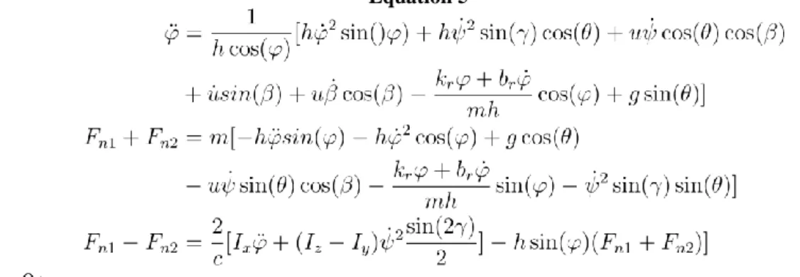
Thanks to the fundamental principle of the dynamic applied to the roll model depicted Fig.1(b), and assuming that
and
, dynamics equation for the roll angle and for the normal forces are given (5):Equation 5
where = + .
Consequently, as soon as the roll angle can be calculated using (5), the LLT can be evaluated thanks to the normal force expressions.
In view of (5), the calculation of requires the knowledge of sideslip angle ( ) whose value depends on cornering stiffnesses
C
f and Cr in view of (3). As quad bikes are expected to move on a natural and slippery ground, grip conditions have an important influence and are moreover varying. Since these variables cannot be measured, their on-line adaptation is then required in order to obtain relevant estimation and prediction of the LLT. Therefore a backstepping observer has been designed to supply on-line their values. Moreover a prediction algorithm is mandatory, if the LLT has to be anticipated in order to prevent the hazardous situations.3 ROLLOVER PREVENTION
3.1 System overview
The developed system aiming at ATV rollover prevention is summarized on Fig.2. It is composed of:
Figure 2: Algorithm overview.
3.1.1 ATV box
The ATV is manually controlled, i.e. the driver specifies the vehicle speed v and steering angle . As described in the introduction, the measured data are the roll/yaw rate, the accelerations, the speed and the steering angle.
3.1.2 Observer box
Contact conditions are then on-line estimated. However for observability reasons (see [10]), the two cornering stiffnesses cannot be estimated separately, and are therefore considered to be equal to a global virtual cornering stiffness Ce. An estimation of the sideslip angle
ˆ
and yaw rateˆ
is alsosupplied. Moreover, the bank angle estimation is integrated into the observer thanks to the measure of the lateral acceleration.
3.1.3 Rollover prevention box
Relying on the measured and observed variables (v, , Ce,
ˆ
andˆ
), future LLT values can bepredicted on-line, in order to prevent the risk of rollover.
The observer and LLT prediction algorithms are more precisely described in the following sections.
3.2 Observer design
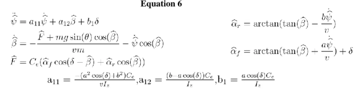
As the front/rear/global sideslip and steering angles can be large, a non-linear system (6) is considered:
Equation 6
Where
ˆ
,ˆ
, ˆrandˆ
f are respectively the observed yaw rate, global sideslip angle, rear sideslipangle and front sideslip angle. Fˆ is named the global lateral force. In order to compute the LLT, and
C
e have to be estimated from (6). With this aim, a backstepping approach composed of 4 steps is proposed. An overview is depicted on Fig.3.Figure 3: Observer overview.
3.2.1 First step “Sideslip angle estimation”
The first step consists in treating as a control input (denoted ), to be designed in order to impose the following dynamic on the observed yaw rate error~:
Equation 7
where is derived from the measured yaw rate. Injecting (7) into the first equation in (6) leads to the following expression for control variable :
Equation 8
under condition a12 0, which is ensured in practice. Since ensures that
ˆ
converges to theactual value supplied by the gyrometer, can be considered as a relevant estimation of the actual global sideslip angle.
3.2.2
Second step“Lateral force reconstruction”
Just as in the first step, F is then treated as a control input (denoted
F
) to be designed to impose thatˆ
~
converges to 0 with the following dynamic:
Equation 9
where is derived from . Injecting (9) into the second equation of (6) leads to the following expression for control variable
F
:Equation 10
Since
F
ensures that converges to the actual value ,F
can be considered as an estimation of the actual lateral force.3.2.3 Third step “Cornering stiffness adaptation”
This step consists in adapting
C
e in order to ensure the convergence of F toF
as defined in equation (6). In view of (6), the adaptation ofC
e cannot be achieved when F=0, which occurs especially when moving straight ahead on a flat ground.The adaptation law used in [10] was stopped during the straight line because of a singularity into the equation (division by δ=0), and it might generate a divergence when the observation restarts.
In order to avoid an adaptation interruption in such a case, a MIT rule adaptation [14] is proposed to obtain the convergence:
Equation 11
with R a strictly positive gain.
As it can be seen on (11), the expression of
C
e is never singular: when moving in straight line on an even ground, the global lateral force (F) tends to zero and consequentlyC
e0
. As a result thecornering stiffness adaptation is frozen in a natural way. This adaptation law (11) does not require to monitor a singularity during straight line motion.
3.2.4 Fourth step “Bank angle estimation”
The principle is to compare the lateral acceleration measured to the one estimated. As the accelerometer is able to measure the constant acceleration like the gravity, the measured lateral acceleration can be modelled into the equation (12).
Equation 12
Moreover, thanks to the yaw and roll representation shown on Fig.1, an estimated lateral acceleration (alongy1
) can be computed:
Equation 13
Finally, the bank angle can be easily estimated with the equation (12) and (13):
3.3 LLT prediction
The previous observer on-line supplies a realist estimation of
C
e, θ describing respectively the grip conditions, the global sideslip and the bank angle. All variables in model equations (3) and (5) are therefore available, and the LLT can then be predicted by integrating these equations over some temporal horizon H. If this prediction reaches a value superior than the threshold (i.e.8
.
0
predictedLLT
), the driver is warned of a rollover risk.More precisely, to perform the integration, the slow-varying variables, i.e. the cornering stiffness
C
eand the bank angle , are supposed constant over the horizon H. On the contrary, the driver’s inputs (i.e. the steering angle and the speed v) have an important influence on the short term evolution of the LLT. Therefore, it is proposed to extrapolate them using a linear function if v and/or present an evolution raising the instability. Otherwise they are kept constant over the horizon H. In this way, the values of the LLT predicted from equations (3) and (5) are at worst overestimated, as it suits for a security device. Precisely, the extrapolation law that has been chosen is:
Equation 15
4 RESULTS
4.1 Setup testbed
Figure 4:MF400H, Massey Fergusson quad bike used for experiments.
In order to validate the observer and the relevance of the LLT prediction proposed in section 3, experimental results are presented. They have been performed with a quad bike MF400H, manufactured by Massey Fergusson and depicted on Fig.4. Its dynamic parameters m ,Iz, kr, br, h, a and b have been preliminary calibrated, and it is equipped with the following sensors:
• a Xsens MTI IMU providing accelerations and angular velocities, • a Doppler radar supplying the linear speed,
• an angular sensor providing the steering angle.
This set of sensors constitutes a low cost perception system (compared to the ATV cost) enabling LLT estimation without requiring for expensive sensors. In addition, dynamometric sensors supplying tire/ground forces have been set up at each wheel. They provide a ground truth, but are not used into the algorithm.
4.2 Experimental results
4.2.1 ATV experimental path
The path described on Fig.5 has been performed on a mixed flat and sloping wet grass ground, at a speed between 3 ms-1 and 5 ms-1. It is composed of a straight line part executed on a 5-15 ° sloping
ground, a U-turn on a partially even area, a second straight line on the same sloping ground, a U-turn on an even area and a third straight line on the same sloping ground.
Figure 5: ATV experiment path.
4.2.2 Estimated bank angle
On Fig.6, the bank angle profile estimated during experiments is depicted. It corresponds to actual slope values recorded ( 15 °) previously by an operator. It then constitutes a satisfactory estimation. According to equation (14), includes the bank angle estimation and the error in the lateral acceleration estimation.
Figure 6: Estimated bank angle.
4.2.3 Observer dynamics
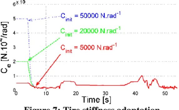
Three experiments have been achieved with different initial conditions for the tire cornering stiffness: 50000 N.rad-1, 20000 N.rad-1 and 5000 N.rad-1. The estimated tire cornering stiffnesses are then represented on Fig.7.
Figure 7: Tire stiffness adaptation.
First, the estimated cornering stiffnesses converge all to the same value. This demonstrates that the choice of the initial condition, which is uneasy, is satisfactorily not crucial. Moreover, the order of magnitude (4000 N.rad-1) is representative of the value for wet grass terrains considering a quad bike.
Secondly, the cornering stiffnesses are convergent despite the first straight line (0-10 s) because of the small slope. The sideslip generated by the slope is sufficient to adapt the cornering stiffness (see (3)).
Thirdly, the cornering stiffnesses are constant during the straight line (0-10 s, 20-37 s and 48-54 s), as expected in section 3.2.3.
Finally
C
e suddenly decreases at 42 s (corresponding to an inversion of the steering angle sign), which is representative of non-linear tire behaviour when slip angle changes quickly.4.2.4 Slope influence on the LLT estimation
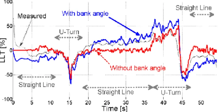
On Fig.8 the LLTs estimated at the current instant (i.e. when H=0 s) with and without the bank angle are depicted (respectively in solid and dashed line) and they are compared to the LLT measured thanks to dynamometric sensors. The quad bike enters the slope at 17 s, then the U-turn occurs between 36 s and 46 s, and finally the vehicle comes back on the slope part.
Figure 8: Experiment results of the LLT estimation.
The LLT estimated without accounting for the bank angle stays around 0 ° in straight line parts, as expected. In this case, is indeed mainly responsible for the LLT. On the contrary, the LLT accounting for the bank angle is almost superposed on the actual LLT, especially during the slope parts.
Nevertheless it can be observed some local inaccuracies, which can be due to the driver’s behavior, neglected in the approach. Since quad bikes are light vehicles, the driver mass is important (for this experiment, the driver’s mass represents 25 % of the total mass), and his behavior has a significant influence. As demonstrated in [15], the position of the driver may change significantly the location of the center of gravity of the overall system and consequently impacts the LLT values. This can explain the LLT overestimation in the first turn-about (12-18 s and 37-43 s).
This experiment shows the importance of taking into account the slope to estimate accurately the LLT. But the driver has to be informed of the risk before it appears, therefore a prediction algorithm is mandatory. The next section discusses the efficiency of the prediction algorithm developed in section 3.3.
4.2.5 Rollover risk indicator
The LLT estimated with the bank angle and the measured LLT are plotted again on Fig.9, respectively in blue and black lines, and compared to the predicted LLT in red:
Figure 9: Experiment results of the LLT prediction.
First, it can be noticed that the three curves are almost superposed in steady state conditions: during the straight line parts and during the constant curves. As expected since the ATV motion is then stationary: the predicted LLT is identical to the current value.
In contrast, during the transient phase (42-45 s) where rollover may occur, the predicted LLT satisfactorily precedes and overestimates the actual LLT.
Consequently, this rollover indicator is able to prevent the lift-off risk for the ATVs on natural ground.
5 CONCLUSION AND FUTURE WORK
This paper proposes an algorithm able to anticipate a rollover risk for ATVs motion on natural ground. An adapted backstepping observer, based on a bicycle model, has been designed in order to estimate the dynamic variables (sideslip angle, cornering stiffness) allowing to adapt to varying conditions and to estimate the slope. Then, relying on a roll model, the LLT is on-line anticipated. The main contributions lie in the consideration of the terrain slope and in the grip condition adaptation. As demonstrated in the experiments, the LLT can be predicted accurately whatever the terrain conditions (sliding, slope). Moreover the sensing equipment is limited to low cost sensors excluding expensive INS or GPS. Nevertheless the driver’s behaviour, which influences the estimated LLT, is not taken into account. Therefore, in order to avoid unnecessary warnings, current developments aim at developing a low cost system which accounts also for the driver’s behaviour.
6 ACKNOWLEDGMENTS
With many thanks for the CCMSA support.
References
[1] “All terrain vehicle enforcement and safety report 2006,” Wisconsin department of natural resources, USA, Tech. Rep., 2007.
[2] CCMSA, “Accidents du travail des salariés et non salariés agricoles avec des quads,” Observatoire des risques professionels et du machinisme agricole, Paris, France, Tech. Rep., 2006.
[3] D. Bevly, J. Ryu, and J. Gerdes, “Integrating INS sensors with GPS measurements for continuous estimation of vehicle sideslip, roll, and tire cornering stiffness,” IEEE Trans. Intell. Transport. Syst., vol. 7, no. 4, pp. 483 –493, 2006. [4] D. Piyabongkarn, R. Rajamani, J. Grogg, and J. Lew, “Development and experimental evaluation of a slip angle
estimator for vehicle stability control,” IEEE Trans. Contr. Syst. Technol., vol. 17, no. 1, pp. 78 –88, 2009.
[5] B. Schofield, T. Hagglund, and A. Rantzer, “Vehicle dynamics control and controller allocation for rollover prevention,” in IEEE International Conference on Control Applications, 2006, pp. 149 –154.
[6] G. Besseron, C. Grand, F. Ben Amar, and P. Bidaud, “Decoupled control of the high mobility robot hylos based on a dynamic stability margin,” in IEEE/RSJ International Conference on Intelligent Robots and Systems (IROS), 2008, pp. 2435 –2440.
[7] K. Ohno, V. Chun, T. Yuzawa, E. Takeuchi, S. Tadokoro, T. Yoshida, and E. Koyanagi, “Rollover avoidance using a stability margin for a tracked vehicle with sub-tracks,” in IEEE/RSJ Safety International Workshop on Security Rescue
Robotics, 2009, pp. 1 –6.
[8] S. Peters and K. Iagnemma, “An analysis of rollover stability measurement for high-speed mobile robots,” in Robotics
and Automation, ICRA, May 2006, pp. 3711 –3716.
[9] M. Spenko, Y. Kuroda, S. Dubowsky, and K. Iagnemma, “Hazard avoidance for high-speed mobile robots in rough terrain,” Journal of Field Robotics, vol. 23, no. 5, pp. 311–331, 2006.
[10] N. Bouton, R. Lenain, B. Thuilot, and P. Martinet, “A rollover indicator based on a tire stiffness backstepping observer : Application to an all-terrain vehicle,” in Int. Conf. on Intelligent RObots and Systems (IROS), Nice, France, 2008. [11] S. Peters, “Stability measurement of high-speed vehicles,” Vehicle System Dynamics, vol. 47, no. 6, pp. 701–720,
2009.
[12] H. B. Pacejka, Tire and vehicle dynamics. Society of Automotive Engineers, 2002.
[13] C. Canudas de Wit and P. Tsiotras, “Dynamic tire friction models for vehicle traction control,” in Decision and
Control, vol. 4, 1999, pp. 3746 –3751.
[14] K. Astrom and B. Wittenmark, Adaptive control (2nd edition). New York: Addison-Wesley, 1994.
[15] N. Bouton, “All-terrain vehicles dynamic stability. new solutions: Application to light vehicles like quad bike,” Ph.D. dissertation, Blaise Pascal University, 2009.