HAL Id: hal-00298987
https://hal.archives-ouvertes.fr/hal-00298987
Submitted on 1 Jan 2001
HAL is a multi-disciplinary open access
archive for the deposit and dissemination of
sci-entific research documents, whether they are
pub-lished or not. The documents may come from
teaching and research institutions in France or
abroad, or from public or private research centers.
L’archive ouverte pluridisciplinaire HAL, est
destinée au dépôt et à la diffusion de documents
scientifiques de niveau recherche, publiés ou non,
émanant des établissements d’enseignement et de
recherche français ou étrangers, des laboratoires
publics ou privés.
Application of a wavelet technique for the detection of
earthquake signatures in the geomagnetic field
L. Alperovich, V. Zheludev, M. Hayakawa
To cite this version:
L. Alperovich, V. Zheludev, M. Hayakawa. Application of a wavelet technique for the detection of
earthquake signatures in the geomagnetic field. Natural Hazards and Earth System Science,
Coperni-cus Publications on behalf of the European Geosciences Union, 2001, 1 (1/2), pp.75-81. �hal-00298987�
and Earth
System Sciences
Application of a wavelet technique for the detection of earthquake
signatures in the geomagnetic field
L. Alperovich1, V. Zheludev2, and M. Hayakawa3
1Dept. of Geophysics and Planetary Sciences, Ramat-Aviv, 69978 Tel-Aviv University, Israel 2School of Computer Science, Tel-Aviv University, 69978 Tel Aviv, Israel
3Dept. of Electronic Engineering, The University of Electro-Communications, Chofu, Tokyo, Japan
Received: 23 May 2001 – Revised: 17 October 2001 – Accepted: 24 October 2001
Abstract. We developed an algorithm especially adapted
to single-station wavelet detection of geomagnetic events, which precede or accompany the earthquakes. The detection problem in this situation is complicated by a great variabil-ity of earthquakes and accompanied phenomena, which ag-gravates finding characteristic features of the events. There-fore we chose to search for the characteristic features of both “disturbed” intervals (containing earthquakes) and “quiet” recordings. In this paper we propose an algorithm for solving the problem of detecting the presence of signals produced by an earthquake via analysis of its signature against the exist-ing database of magnetic signals. To achieve this purpose, we construct the magnetic signature of certain earthquakes using the distribution of the energies among blocks, which consist of wavelet packet coefficients.
1 Introduction
It is expected that local geomagnetic disturbances caused by under the surface seismic and tectonic activity contribute substantially to the total geomagnetic field, including magne-tospheric and antrophogenic fields. Through the interaction of the flux of interporous conductive liquid with the field of microcracks, these disturbances can be generated by such a flux (Gershenzon et al., 1993; Molchanov 1995). To achieve a better understanding of the sources, properties and be-haviour of the local perturbations, it is important, therefore, to learn to recognize these disturbances. Alperovich and Zhe-ludev (1998) suggested a method based on the detection of the differences in the spatial distributions of magnetospheric and tectonogenic perturbations. In addition to conventional wavelet analysis, wavelet packet transforms of simultaneous recordings of geomagnetic signals from a number of obser-vatories were also employed. The coefficients obtained were subjected to either thresholding or mutual comparison in
or-Correspondence to: L. Alperovich
der to reveal the events we were looking for. The proce-dure of comparison of simultaneous wavelet coefficients al-lowed for the dection of two types of perturbations spreading from the epicentral zone. The technique of stationary wavelet transform has been used for the best time-domain localiza-tion of events.
It was discovered that a quake produces geomagnetic dis-turbances of two types. The first type consists of the low-frequency oscillations with periods ranging within several hours. The second type consists of relatively high-frequency oscillations with periods of about 10 min. The low-frequency oscillations are propagating along the ground surface with the velocity of sound. The high-frequency ones are radiat-ing outward from the seismoactive region at a rate of about 5 km/s. The aim of this paper is to contribute to the research of geomagnetic perturbations caused by a subsurface source using single-point, long-term geomagnetic observations in a seismic active region. We supply a new approach to the prob-lem of the search of earthquake precursors based on the cre-ation of a wavelet signature of the observed field for quiet periods and the period preceding an earthquake. As original data, we used 3-component recordings of a geomagnetic ob-servatory Kagoshima (58.5◦N, 130.7◦E) within a 6-month
period with a 1 s sampling rate (Yumoto et al., 1992). Within this period two significant earthquakes (M = 6.2, 26 March 1997/ 08:31 GMT, 32.0◦N, 130.3◦E; M = 6.1, 13 May 1997/ 05:38 GMT, 31.9◦N, 130.3◦E) occurred. We used data from the World Data Center A for Seismology (National Earthquake Information Center (http://neic.usgs.gov/epic)).
2 General approach
We tried to develop an algorithm which could distinguish be-tween a magnetic field recorded just before an earthquake and the field recorded within a quiet time interval. Obvi-ously, it is a classification problem. The basic assumption is that the general signature of the geomagnetic field in the given region could be obtained as a combination of energies
76 L. Alperovich et al.: On wavelet geomagnetic signature of an earthquake
10
Signal f
Low frequency block w1 = 2↓Hf
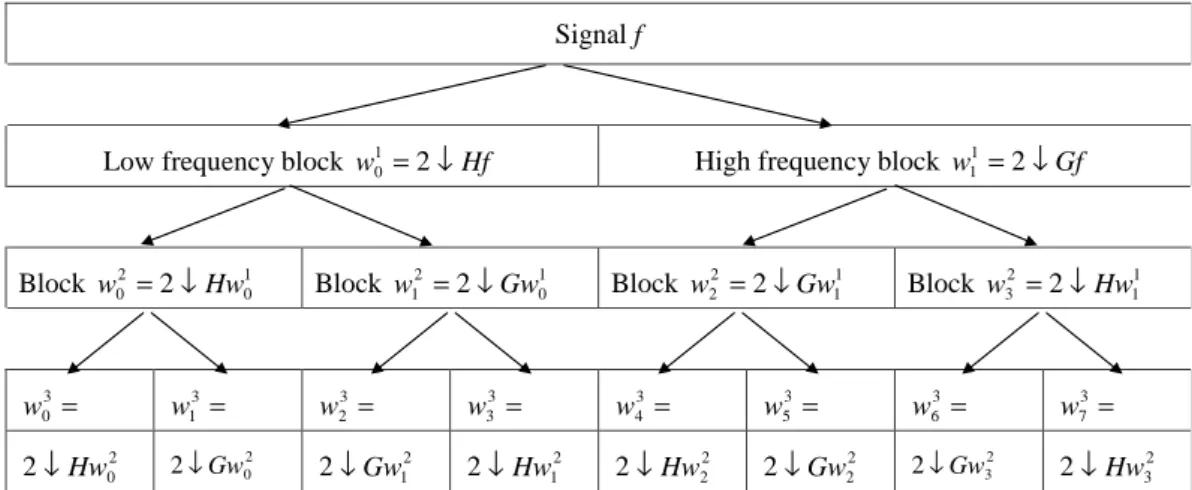
0 High frequency block w = 2↓Gf 1 1 Block 1 0 2 0 2 Hw w = ↓ Block 1 0 2 1 2 Gw w = ↓ Block 1 1 2 2 2 Gw w = ↓ Block 1 1 2 3 2 Hw w = ↓ = 3 0 w 3 = 1 w 3= 2 w 3= 3 w 3= 4 w 3= 5 w 3 = 6 w 3 = 7 w 2 0 2↓Hw 2↓Gw20 2 1 2↓Gw 2 1 2↓Hw 2 2 2↓Hw 2 2 2↓Gw 2↓Gw32 2 3 2↓Hw Figure 1.
Fig. 1. Flow of the wavelet packet transform. The partition of the frequency domain corresponds approximately to the location of the blocks
in the diagram. There are seven levels of the subdivision scheme for the frequency band on different levels L and block numbers Nblock.
inherent in a small set of the most essential blocks of the wavelet packet decompositions of the recorded signals (see Appendix A). We assume a remarkable disturbance of this configuration before and during the event of earthquake.
A crucial factor in having a successful classification is to construct signatures built from characteristic features that en-able one to discriminate among classes. Multiscale wavelet analysis of recorded signals provides a promising methodol-ogy for this purpose. Recently, several wavelet-based tech-niques for feature extraction were developed. We men-tion the Local Discriminant Bases (LDB) algorithm (Saito and Coifman, 1995), Discriminant Pursuit (Buckheit and Donoho, 1995) and the Matching Pursuit method (Mallat, 1998) for the construction of the wavelet packet bases that separate classes of signals. The LDB algorithm was applied to classification of some geological phenomena (Saito and Coifman, 1997).
In the final phase of the process, in order to identify the earthquake signatures of the predetermined classes of signals, we used conventional classifiers such as Linear Discriminant Analysis (LDA) (Saito and Coifman, 1995) and Classification and Regression Trees (CART) (Breiman, 1993). For training purposes, we use a set of signals with known membership. From this set, we select a few blocks which discriminate efficiently between the given classes of signals. Then, we apply the wavelet packet transform on the signal to be classified. We use as its characteristic fea-tures the wavelet packet coefficients normalized by the en-ergy contained in the selected blocks. Finally, we submit the extracted features to one of the classical classifiers, who is appropriately trained beforehand, and decides which class this signal belongs to.
The algorithm is centered on two basic issues: (1) selec-tion of the discriminant blocks of the wavelet packet coeffi-cients; (2) discrimination among the signals.
2.1 Selection of discriminant blocks
We used Spline and Coiflet wavelet transforms. These filters reduce the overlapping among frequency bands associated with different decomposition blocks. Initially, we gathered as many recordings as possible for each class, which have to be separated (including to an earthquake and “quiet” inter-val). Then, we prepared from each selected recording, which belongs to a certain class, a number of overlapping slices of length n = 2J samples each, shifted with respect to each other. These groups of slices form the training set for the search of discriminant blocks.
We use the l2 or l1 norms to measure the energy in the
block. Then, the wavelet packet transform is applied up to scale m on each slice of length n from a given class Cl,
l =1, 2. This procedure produces mn coefficients arranged into 2m+1−1 associated with different frequency bands (see Fig. 1).
The slice is decomposed. The “energies” of each block are calculated in accordance to the chosen measure. As a result we obtain, to some extent, the distribution of the “en-ergies” of the slice over various frequency bands of widths from NF/2 to NF/m, where NF is the Nyquist frequency.
In our case,
NNyquist=0.5sample frequency=fmax=0.5 Hz.
The whole frequency range is divided by 2L sub-intervals (blocks). So the maximal frequency fblock of the block of
number Nblockis
fblock=
Nblock·fmax
2N .
Figure 1 demonstrates a subdivision scheme of the whole fre-quency range for L = 7 to allow us to go to a finer resolution of the wavelet packet transform. The energy is presented by
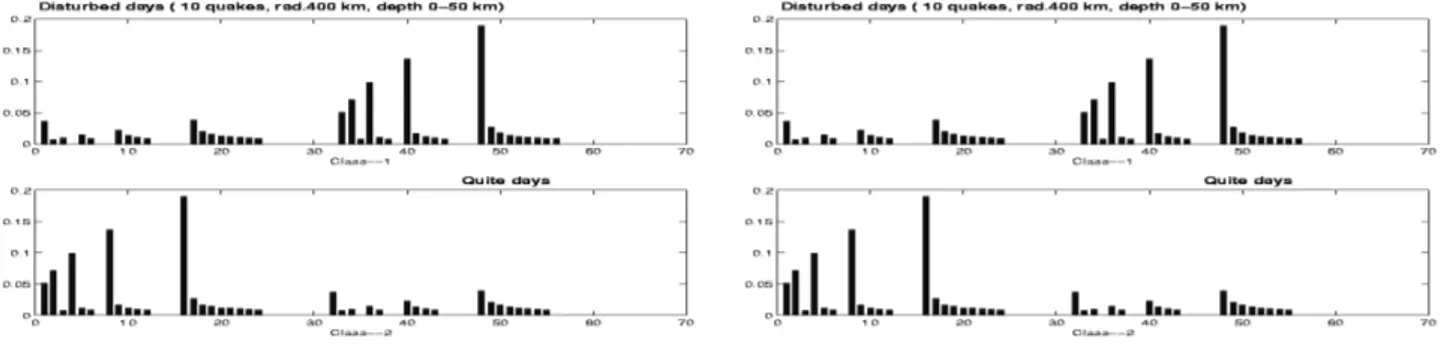
11 Figure 2
Fig. 2. Energy map for 5 decomposition levels of a two-class problem (left picture) and the difference in class C1(10 earthquakes, radius
400 km, depth 0–50 km) and class C2(seismic “quiet” days) maps (right picture). The length of a slice is n = 1024 samples.
an energy vector Eilof length 2m+1−1. The energy vectors along the training set of the class are averaged:
El = 1 M M X i=1 Eil.
The average energy map Elindicates how the distribution of the “energies” among the various blocks of the decomposi-tion and frequency bands, respectively, is taking place within the whole class Cl. The left picture in Fig. 2 displays a typ-ical energy map for 5 decomposition levels of a two-class problem. The heights of the bars indicate the normalized en-ergy of each of the 63 decomposition blocks.
2.2 Discriminant power and selection of discriminating blocks
The average energy map yields some sort of characterization for the chosen class, but it is highly redundant. To gain a more concise and meaningful representation of the class, we select the most discriminating blocks. One possible way to do so is the following. First, note that for a two-class prob-lem, the difference between two maps provides some insight into the problem (Fig. 2, right). The differences for most blocks are near zero. It means that they are of no use for dis-crimination, unlike a few blocks with large values in their dif-ferences. Therefore, the term-wise difference (absolute val-ues) of the energy maps serves as the discriminant power map for the decomposition blocks DP (1, 2) = E1−E2 . As a result of the operations described above, we discover a rela-tively small set of decomposition blocks, such that the distri-bution of energies amongst them characterizes the classes to be distinguished.
2.3 Preparation of the reference set
Initially, we chose a number of recordings that belong to the classes to be distinguished, from which we form the refer-ence set. These recordings are sliced similarly to that which was used for the preparation of the training set. For a certain class, we form a number of overlapping slices each of length nform from each selected recording belonging to the class. These are shifted with respect to each other by s samples.
12 Figure 3 3 0 0 5 0 0 7 0 0 9 0 0 R a d iu s , k m 6 1 0 1 4 1 8 2 2 N u m b e r of ear thquak es
Fig. 3. Dependency of numbers of earthquakes of magnitude range
of M = 5.07.0 on distance from Kagoshima for January–May, 1997.
Then, we apply the wavelet packet transform up to level m on each row of this matrix. After the decomposition, we cal-culate only the “energies” of the blocks that were selected before. We do the same for both classes. The reference sets are used for two purposes: (1) as pattern sets for LDA, (2) as training sets for building CART.
The construction of the classification tree is done by a bi-nary split of the space of input patterns so that once a appears in the subspace Xk, its membership could be predicted with
a reasonable reliability. The basic idea with the split is that the data in each descendant subset is more “pure” than the data in the parent subset.
After the construction of the classification tree, with pat-tern sets for LDA, we are in a position to classify test signals.
78 L. Alperovich et al.: On wavelet geomagnetic signature of an earthquake
13
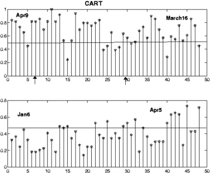
Figure 4.
Fig. 4. The top picture illustrates the
classification rate for the signals of class
C1(16 March, 05:51, M = 5.7, ϕ =
35, λ = 137; 9 April, 07:02, M = 5.4,
ϕ =26, λ = 128) and the bottom
pic-ture illustrates the signals of C2class.
Each (*) in the picture corresponds to a 1 h interval. Vertical lines are the ra-tio h of the number of vectors attributed
incorrectly to the Cl class (l = 1, 2) to
the total number of the vectors associ-ated with the signals of the l-th class.
So, if 0 < hl <0.5, then the number of
correct answers prevails over the num-ber of wrong ones, and the signal is well
classified. If hl =0, then the signal is
classified completely. If 0.5 < hl <1,
then the signal is misclassified.
3 Results
We conducted two series of experiments: (1) classification of signals emitted by earthquakes; and (2) discrimination be-tween signals emitted by earthquakes and the background. We tested various families of wavelet packets and various norms for the feature extraction and various combinations of features presented to the LDA and CART classifiers. The best results were achieved with wavelet packets based on Coiflet 5 filters with 10 vanishing moments and splines of the order 8. LDA classifiers in most experiments outperformed CART.
We processed the signals using the scheme explained above. For the selection of the discriminant blocks we used geomagnetic recordings around the time of 21 earthquakes appearing at distances up to 1000 km from Kagoshima (Yu-moto et al., 1992). Figure 3 shows the dependency of the number of earthquakes with magnitudes of 5–8 and depth ranges of 0–100 km in distance. The recording is processed under sliding overlapped windows of size n = 1024. The window was shifted along the signal with a step of s = 128 samples. Each window was processed by the wavelet packet transform up to the 6th level. The best results were achieved when we used spline 8 wavelet packets and either l1 or l2
norms as the “energy” measure for the blocks. As a result, we selected various sets of discriminant blocks.
The top picture of Fig. 4 illustrates the classification rate for the signals of class C1 (“disturbed” days: 16 March, 05:51 GMT, M = 5.7, ϕ = 35, λ = 137; 9 April, 07:02 GMT, M = 5.4, ϕ = 26, λ = 128) and the bottom picture illustrates the signals of C2 class: 6 January (num-bers 0–24) and 5 April (24–48). Each (*) in the picture cor-responds to a single 1 h interval of class C1. Its height, h1,
may range from 0 to 1 and is
h1= K
l
Kl c
where Kl is the total number of s W (i, :) associated with the signal and Kcl is the number of the s W (i, :) attributed correctly to the class Cl. So, if hl = 0, then the signal Sl is completely classified. If 0 < h < 0.5, then the number of correct answers prevails over the number of wrong ones, and the signal is classified. The closer hl gets to 0, the more reliable the answer. If hl =0.5, then the number of correct answers is equal to the number of wrong ones, and the signal is non-classified. And, finally, if 0.5 < hl < 1, then the signal is misclassified.
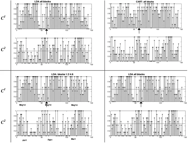
In Fig. 5, we present the results of training and classifica-tion. The following parameters were used: Spline 6 wavelets; CART and LDA classifiers. The signals were decomposed up to the 7th level the chosen wavelet was close to rectan-gular. We took the magnetograms of 25–27 March (“dis-turbed” days, class C1) and 9–11 March (“quiet” days, class C2) as the training signals. We submitted to be classified new disturbed and quiet days using the same training signals as before. The signals of the C1class were 12–14 May 1997 (M = 5.6, 13 May, 05:38 GMT). The epicenter was almost at the same point as the 26 March earthquakes. For the sig-nals of the C2class, we choose 1 January, 1 February and 1 March. In the results presented in the left pictures of Fig. 5, we used 1:2, 4:6 blocks and in the right picture, all blocks. For a decision, we used the Classification and Regression TREE (CART) classifiers in the top panel and the Linear Dis-criminant Analysis (LDA) in the bottom panel. The upper picture in each panel corresponds to the disturbed period and the bottom picture corresponds to the quiet period.
14
C
1C
2C
1C
2Figure 5.
Fig. 5. The results of training and classification. The following parameters were used: Spline 6 wavelets; CART and LDA classifiers. The
signals were decomposed up to the 7th level. As the training signals, we took recordings on 25–27 March (“disturbed” days, class C1) and
9–11 March (“quiet” days, class C2). We submitted to be classified new “disturbed” and “quiet” days using the training signals as before.
The signals of the C1class were 12–14 May 1997 (M = 5.6, 13 May, 05:38). The epicenter was almost at the same point as the 26 March
earthquakes. For the signals of the C2class, we chose 1 January, 1 February and 1 March. In the results presented in the left pictures, we
used 1:2, 4:6 blocks and in the right picture, all blocks. For the decision we used the Classification and Regression TREE (CART) classifiers
in the top panel and the Linear Discriminant Analysis (LDA) in the bottom panel. The upper picture in each panel corresponds to the C1
class and bottom picture corresponds to the C2class.
We can see that the classification rate for the signals of class C2are less than 0.5, in general, i.e. both classifiers cor-rectly classify the quiet magnetograms. At the same time the majority of the C1signals are misclassified. The classifiers cannot separate them from the C2signals, except for the 3–4 hour period before the M = 5.6 26 March earthquake. Here the substantial fraction signals are well classified (LDA clas-sifier). A performed numerical experiment demonstrates that indeed there is something irregular in the energy signature of the geomagnetic variations recorded closely (around 20 km) to the earthquake epicenter.
One can see that the classification procedure separates the observed magnetic field into two classes with a level of confi-dence just on the isolated parts of recordings, namely before 1 day, and 4 hours before the earthquake. Common features
appear in the geomagnetic field preceding both the 26 March and 13 May earthquakes. The anomalies occupy a wide pe-riod range (from 10 s to 250 s). Narrowing of the interval and excluding the low-frequency band degrades the classifi-cation (see, for comparison, the right panel of Fig. 5 where we used all blocks and the left panel where rather high fre-quency blocks were used).
On the next stage, we constructed a training tree for the C1class, including new time intervals corresponding to mo-ments of earthquakes taken from different levels of remote-ness. The results of the classification did not change until the radius up to 300 km from Kagoshima when we included six 3-day intervals containing five additional earthquakes. The following increase of the radius leads to a degradation of the classification.
80 L. Alperovich et al.: On wavelet geomagnetic signature of an earthquake Discovering the localization of the geomagnetic signature
does not mean directly locality of the generated signals, since a signal can spread away from the source on large distances. In doing so, the energetic portrait which is a distinctive rela-tionship between the energies on different levels and blocks, can be lost, and an emitted signal forgets about the source. For example, Alperovich and Zheludev (1998) applied the wavelet-based approach to the US geomagnetic network data and extracted the wave components by aligning the arrival time of each observation point. Oscillations within the range from 10 min to a few hours, 5 hours and 2 days prior to the occurrence of the strong Loma Prieta earthquake, have been revealed. The main feature of the discovered variations is spreading northward from the epicentral zone. Direct com-parison of the results from Alperovich and Zheludev (1998) with field geomagnetic observations close to the epicenter (see Hayakawa et al., 1996; Merzer and Klemperer, 1997; Ismaguilov et al., 2001; and references herein) confirm our conclusion regarding the time and characteristic time-scale of the precursors.
Appendix A Wavelet packet transforms
The result of the application of the m-level wavelet packet transform to a signal f of length n = 2J is a set of mn correlation coefficients of the signal with shifted versions of 2m+1−2 basic waveforms: the wavelet packets. The trans-form is implemented through iterated application of a con-jugate pair of low (H ) and high (G) pass filters followed by downsampling. In the first decomposition step, the fil-ters are applied to the signal f and after downsampling, the result has two blocks, w01and w11, of the first scale, each of size n/2. These blocks consist of the correlation coefficients of the signal with 2-sample shifts of the low-frequency fa-ther wavelet and high-frequency mofa-ther wavelet related to the filters (H ) and (G), respectively. The block w01contains the coefficients necessary for the reconstruction of the low-frequency component of the signal. Due to the orthogonality of the filters, the energy (l2 norm) of the block w01is equal
to that of the component W01. Similarly, the high-frequency component W11can be reconstructed from the block w11. In that sense, each decomposition block is linked to a certain half of the frequency domain of the signal. The signal f is the sum:
f = W01+W11.
Both blocks w01 and w11 are stored at the first level and at the same time, both are processed by a pair of filters, H and G, which generate four blocks w02, w12, w22, w23 in the sec-ond level. These are the correlation coefficients of the signal with 4-sample shifts of the four new waveforms whose spec-tra split the frequency domain into four parts. All of these blocks are stored in the second level and transformed into eight blocks in the third level, etc. The involved waveforms are well localized in time and frequency domains. Their spectra form a refined partition of the frequency domain (into
2mparts at the level m). Correspondingly, each block of
co-efficients of the wavelet packet transform describes the com-ponent of the signal f related to a certain frequency band. The l2norm of this block is equal to the norm of the
compo-nent.
There are many wavelet packet libraries. They differ from each other by their generating filters H and G, the shape of the basic waveforms and the frequency content. It was im-portant for our investigation to have refined frequency resolu-tion. Therefore, we have chosen the wavelet packets derived from the splines of the 8th order.
Acknowledgements. We are grateful to Dr. K. Yumoto and the
members of the 210◦magnetic meridian team who contributed to
the successful operation of the Kagoshima station (Yumoto et al., 1992).
References
Alperovich, L. and Zheludev, V.: Wavelet transform as a tool for de-tection of geomagnetic precursors of earthquakes, J. Phys. Chem. Earth, 23, 965–967, 1998.
Averbuch, A. Z., Hulata, E., Zheludev, V. A., and Kozlov, I.: A wavelet packet algorithm for classification and detection of mov-ing vehicles, Multidimensional Systems and Signal Processmov-ing, 12, 9–31, 2001.
Breiman, L., Friedman, J. H., Olshen, R. A., and Stone, C. J.: Clas-sification and Regression Trees, Chapman and Hall, Inc., New York, 1993.
Buckheit, J. and Donoho, D.: Improved linear discrimination using time-frequency dictionaries, Proc. SPIE, 2569, 540–551, 1995. Coifman, R. R., Meyer, Y., and Wickerhauser, M. V.: Adapted
waveform analysis, wavelet-packets, and applications, In Pro-ceedings of ICIAM’91, SIAM Press, Philadelphia, 41–50, 1992. Eom, K. B.: Analysis of acoustic signatures from moving ve-hicles using time-varying autoregressive models, Multidimen-sional Systems and Signal Processing, 10, 357–378, 1999. Fisher, R. A.: The use of multiple measurements in taxonomic
prob-lems, Ann. Eugenics, 7, 179–188, 1936.
Gershenzon, N. I., Gohberg, M. B., Karakin, A. V., Petviashvili, N. V., and Rykunov, A. L.: Modelling the connection between earth-quake preparation process and crustal electromagnetic emission, Phys. Earth. Planet. Inter., 77, 85–95, 1993.
Hayakawa, M., Kawate, R., Molchanov, O. A., and Yumoto, K.: Re-sults of ultra-low-frequency magnetic field measurements during the Guam earthquake of 8 August 1993, Geoph. Res. Lett., 23, 241–244, 1996.
Ismaguilov, V. S., Kopytenko, Yu. A., Hattori, K., Voronov, P. M., Molchanov, O. A., and Hayakawa, M.: ULF magnetic emissions connected with under sea bottom earthquakes, GRA3, 8957, Nat-ural Hazards, Geophys. Res. Abst., 3, 2001.
Mallat, S. and Zhang, Z.: Matching pursuit with time-frequency dictionaries, IEEE Trans. Sign. Proc., 41, 3397–3415, 1993. Mallat, S.: A wavelet tour of signal processing, Acad. Press, 1998. Merzer, M. and Klemperer, S. L.: Modeling low-frequency
mag-netic field precursors to the Loma Prieta earthquake with a pre-cursory increase in fault-zone conductivity, Pure and Appl. Geo-phys., 150, 217–248, 1997.
Molchanov, O. A. and Hayakawa, M.: Generation of ULF electro-magnetic emissions by microfracturing, Geoph. Res. Lett., 22, 3091–3094, 1995.
Saito, N. and Coifman, R. R.: Local discriminant bases and their application, J. Mathematical Imaging and Vision, 5, 337–358, 1995.
Saito, N. and Coifman, R. R.: Improved local discriminant bases using probability density estimation, Proc. Am. Statist. Assoc., Statistical Computing Section, 5, 312–321, 1996.
Saito, N. and Coifman, R. R.: Extraction of geological information from magnetic well-logging waveforms using time-frequency wavelets, Geophysics, 62, 1921–1930, 1997.
Yumoto, K., Tanaka, Y., Oguti, T., Shiokawa, K., Yoshimura, U., Isono, A., Fraser, B. J., Menk, F. W., Lynn, J. W., Seto, M.,
and 210◦ MM magnetic observation group: Globally
coordi-nated magnetic observations along 210◦magnetic meridian
dur-ing STEP period-1, Preliminary results of low-latitude Pc3’s, J. Geomagn. Geoelectr., 44, 261–276, 1992.