HAL Id: hal-00296428
https://hal.archives-ouvertes.fr/hal-00296428
Submitted on 5 Feb 2008
HAL is a multi-disciplinary open access
archive for the deposit and dissemination of
sci-entific research documents, whether they are
pub-lished or not. The documents may come from
teaching and research institutions in France or
abroad, or from public or private research centers.
L’archive ouverte pluridisciplinaire HAL, est
destinée au dépôt et à la diffusion de documents
scientifiques de niveau recherche, publiés ou non,
émanant des établissements d’enseignement et de
recherche français ou étrangers, des laboratoires
publics ou privés.
tropical lower stratospheric water vapor
S. Dhomse, M. Weber, J. Burrows
To cite this version:
S. Dhomse, M. Weber, J. Burrows. The relationship between tropospheric wave forcing and tropical
lower stratospheric water vapor. Atmospheric Chemistry and Physics, European Geosciences Union,
2008, 8 (3), pp.471-480. �hal-00296428�
Atmos. Chem. Phys., 8, 471–480, 2008 www.atmos-chem-phys.net/8/471/2008/ © Author(s) 2008. This work is licensed under a Creative Commons License.
Atmospheric
Chemistry
and Physics
The relationship between tropospheric wave forcing and tropical
lower stratospheric water vapor
S. Dhomse, M. Weber, and J. Burrows
Institute of Environmental Physics, University of Bremen, Bremen, Germany
Received: 15 August 2006 – Published in Atmos. Chem. Phys. Discuss.: 28 September 2006 Revised: 13 March 2007 – Accepted: 4 January 2008 – Published: 5 February 2008
Abstract. Using water vapor data from HALOE and SAGE
II, an anti-correlation between planetary wave driving (here expressed by the mid-latitude eddy heat flux at 50 hPa added from both hemispheres) and tropical lower stratospheric (TLS) water vapor has been obtained. This appears to be a manifestation of the inter-annual variability of the Brewer-Dobson (BD) circulation strength (the driving of which is generally measured in terms of the mid-latitude eddy heat flux), and hence amount of water vapor entering the strato-sphere. Some years such as 1991 and 1997 show, however, a clear departure from the anti-correlation which suggests that the water vapor changes in TLS can not be attributed solely to changes in extratropical planetary wave activity (and its effect on the BD circulation). After 2000 a sudden decrease in lower stratospheric water vapor has been reported in ear-lier studies based upon satellite data from HALOE, SAGE II and POAM III indicating that the lower stratosphere has become drier since then. This is consistent with a sudden rise in the combined mid-latitude eddy heat flux with nearly equal contribution from both hemispheres as shown here and with the increase in tropical upwelling and decrease in cold point temperatures found by Randel et al. (2006). The low water vapor and enhanced planetary wave activity (in turn strength of the BD circulation) has persisted until the end of the satellite data records. From a multi-variate regres-sion analysis applied to 27 years of NCEP and HadAT2 (ra-diosonde) temperatures (up to 2005) with contributions from solar cycle, stratospheric aerosols and QBO removed, the en-hancement wave driving after 2000 is estimated to contribute up to 0.7 K cooling to the overall TLS temperature change during the period 2001–2005 when compared to the period 1996–2000. NCEP cold point temperature show an average decrease of nearly 0.4 K from changes in the wave driving, which is consistent with observed mean TLS water vapor changes of about −0.2 ppm after 2000.
Correspondence to: S. Dhomse
1 Introduction
Stratospheric water vapor plays an important role in deter-mining radiative and chemical properties of the middle at-mosphere. As a primary source of odd hydrogen in the stratosphere, it controls ozone loss through gas phase chem-istry. In addition, the coupling processes between HOxand
NOx/ClOx affect ozone destruction by other catalytic
re-action cycles and heterogeneous chemistry on polar strato-spheric clouds responsible for spring time polar ozone loss. An increase in stratospheric WV could have serious impli-cations on the future evolution of the ozone layer (Shindell et al., 1999; Tabazadeh et al., 2000; Stenke and Grewe, 2005) and, therefore, delay ozone recovery (Shindell, 2001). The longest in situ time series of stratospheric water vapor mea-surements is available from balloon meamea-surements in Boul-der, Colorado (40◦N, 105◦W). The water vapor volume mix-ing ratios (VMRs) in the lower stratosphere above Boul-der have been increasing by about 1% per year since 1981 (Oltmans et al., 2000). Trends in stratospheric water vapor above 18 km are, however, lower in the satellite data records (SPARC, 2000; Randel et al., 2004b).
Initially it was believed that methane oxidation might have contributed to rising levels of water vapor in the stratosphere. The observed changes in stratospheric methane at most con-tribute only about one third to the water vapor trend (SPARC, 2000). Another important source of stratospheric water va-por variability are changes in the tropical tropopause temper-atures which determine the water vapor VMRs of the air en-tering in to the stratosphere (Brewer, 1949; Rosenlof, 2003). But tropical tropopause temperatures have not increased as would be needed for a stratospheric H2O increase (SPARC,
2000; Randel et al., 2004b).
Any changes in tropical tropopause temperatures is likely to be associated in part with with changes in BD circula-tion. The BD circulation is primarily driven by breaking of tropospherically generated planetary waves (e.g. Rossby wave) in the extratropical stratosphere. The influence of
the planetary wave activity on the stratospheric circulation is generally explained in terms of the “downward control prin-ciple” (Haynes et al., 1991), which means that the ascent or descent of air-masses at certain altitudes is determined by the momentum (as expressed by the convergence of the Eliassen-Palm flux) deposited above it. Mass balance requires that the descent of air from the stratosphere down to the troposphere at high latitudes and ascent of tropospheric air into the trop-ical stratosphere is accompanied by horizontal mixing. De-scending airmasses at high latitudes undergo adiabatic com-pression thereby increasing polar stratospheric temperatures away from the radiative equilibrium (Newman et al., 2001), while the ascent at low latitudes lowers stratospheric tem-peratures by adiabatic expansion (Yulaeva et al., 1994). The eddy heat flux is directly proportional to the vertical com-ponent of EP flux and, therefore a useful estimate of the EP flux convergence. It has been linked to changes in strato-spheric ozone, temperatures at high latitudes and tropics, as well as chlorine activation inside the polar vortex (Yulaeva et al., 1994; Fusco and Salby, 1999; Newman et al., 2001; Weber et al., 2003).
Most of the studies earlier studies related to stratospheric water vapor are focused on tropical processes such as over-shooting, QBO, tropical upwelling or cold point tempera-tures near tropical tropopause region. For e.g. the relation-ship between tropical cold point temperatures and strato-spheric water vapor is well established. Using trajectory calculations and a cold point based dehydration mechanism, F¨uglistaler et al. (2005) showed good agreement between modeled and observed stratospheric water vapor VMRs in the TTL. They concluded that an 1 K change in cold point temperatures lead to about 0.5 ppm change in water vapor VMRs. On long term scale, F¨uglistaler and Haynes (2005) concluded that most of the inter-annual variability in the 1990s is dominated by QBO and to some extent by El Ni˜no. Randel et al. (2006) showed that the seasonal variations in water vapor VMRs in TLS show a correlation (r=0.73) with changes in cold point temperatures (with lag of 2 months). Randel et al. (2004b, 2006) showed that the observed de-creases in stratospheric water vapor VMRs since 2000 are consistent with decreases in tropical cold point temperatures and enhanced tropical upwelling between 20◦N–20◦S. They also showed that temperature changes in the TTL can be associated with radiative feedback from tropical ozone de-crease near the tropical tropopause (Randel et al., 2006).
Randel et al. (2006) demonstrated the significant correla-tion between tropical upwelling and cold point temperature in the TTL as well as water vapor VMRs in the tropical lower stratosphere, despite the fact that ascent velocities are associ-ated with high uncertainties since it is a highly derived quan-tity from the meteorological analyses. They also showed that the period after 2000 with lower water vapor concentrations (Randel et al., 2004b; Nedoluha et al., 2002) can be linked to an increase in the average strength of the Brewer-Dobson circulation after 2000 as compared to a five year period
be-fore. The relationship between cold point temperature and tropical upwelling (Randel et al., 2006), on one hand, and the expected correlation between tropical upwelling and mid-latitude eddy heat flux, on the other hand, suggest a close re-lationship between the inter-annual variablity of TLS water vapor and eddy heat flux similar to that observed for strato-spheric ozone (Randel et al., 2002b; Weber et al., 2003). In this paper we are interested in the question of how well the year-to-year variability in the tropical stratospheric water va-por can be associated with variations in the BD circulation strength (here expressed by the winter-spring time cumula-tive extratropical eddy heat flux) since the start of the satel-lite records in 1984 (SAGE II, HALOE). We also attempt to estimate the potential contribution of the BD circulation to TLS and cold point temperature changes after 2000 from a regression analysis covering 27 years of temperature data.
After a brief introduction on the used water vapor data sets and meteorological analyses (Sect. 2), we look at the inter-annual variability in tropical water vapor and BD circulation (Sect. 3). The drop in stratospheric water vapor after 2000 (Randel et al., 2004b, 2006) in connection with the enhanced planetary wave activity and TLS temperature changes is dis-cussed in Sect. 4.
2 Data
2.1 Water vapor data
Currently only a few good quality stratospheric water vapor data sets are available for long term analysis. Near global water vapor measurements are provided by the Stratospheric Aerosol and Gas Experiment II (SAGE II, 1984–2005) and the Halogen Occultation Experiment (HALOE, 1992–2005). Both instruments and POAM III (1998–2005, see below) ceased operating by the end of 2005. All three instruments use the solar occultation technique to measure attenuated so-lar radiation through Earth’s limb at discrete wavelengths, which is then inverted to retrieve concentrations of various trace gases in the atmosphere. For water vapor retrieval the primary channel used in SAGE II is near 935 nm (Thoma-son et al., 2004), while HALOE uses radiances near 6.61 µm (Russell et al., 1993). Both instruments provide approxi-mately 15 sunrise and 15 sunset measurements per day. For the retrieval below 35 km, both HALOE and SAGE II use temperature profiles from NCEP. For complete global cover-age (except for the highest latitudes) both instruments need about 1 to 1.5 months.
In this study SAGE II V6.2 data were analyzed . The vertical sampling of the SAGE II water vapor profile is about 0.5 km with a vertical resolution of 1 km. Although there are significant improvements compared to earlier ver-sion of the WV data, there are still some problems dur-ing years with high stratospheric aerosol loaddur-ing (Thoma-son et al., 2004). Taha et al. (2004), suggested that water
S. Dhomse et al.: BD circulation and water vapor 473 vapor profiles with aerosol extinction coefficient at 1020 nm
greater than 2×10⁻⁴km−1are not reliable and they were
re-moved from our analysis, thus excluding the periods 1984– 1985 and 1992–1994. HALOE V19 data were obtained from http://haloedata.larc.nasa.gov/. HALOE has an instan-taneous field of view of about 1.6 km and a vertical resolution varying between 2 and 3 km. However, the data were inter-polated to a 0.3 km grid for retrieval purposes. It should be noted that both SAGE II and HALOE measurements show largest uncertainties near the TTL region due to measure-ment geometry (SPARC, 2000). The water vapor profiles have been weighted with the inverse of square of measure-ment errors when calculating monthly zonal means. This means that measurements with smaller errors is given higher weights in the averaging procedure.
In addition to SAGE II and HALOE, the Polar Ozone and Aerosol Measurement (POAM III, 1998–2005) water vapor version 4 data set has been used in this study (Nedoluha et al., 2002). POAM III also measures in solar occultation mode, but water vapor profiles are only available for higher lati-tudes. Data have been obtained from www.cpi.com/ and the vertical resolution is about 1 km.
In this study, monthly mean zonal mean water vapor values from the satellite data were calculated when at least five ob-served profiles in a given latitude band were available. Data gaps in months with less than five profiles were filled by val-ues obtained from a harmonic analyses of the time series con-taining annual and semi-annual terms.
2.2 Meteorological data
Meteorological data used here are primarily from the Na-tional Center for Environmental Prediction (NCEP)/NaNa-tional Center for Atmospheric Research (NCAR) reanalysis model (Kalnay et al., 1996). Data at six hour intervals on a 2.5◦×2.5◦grid were obtained from www.cdc.noaa.gov/cdc/ data.ncep.reanalysis.pressure.html. The major advantage of NCEP reanalysis data is that the assimilation system remains unchanged, although changes in the quality of assimilated data and their availability strongly influences the analyses (for detailed discussion see Randel et al., 2004a). The eddy heat flux is calculated using daily temperature and wind data as described in Randel et al. (2002b). The monthly mean eddy heat flux data have been derived from daily values. In addition to the available isobaric analysis fields, cold point temperatures have been derived from NCEP.
Another relevant meteorological data are the 40-year re-analysis (ERA-40) (Uppala et al., 2005) and ECMWF op-erational analysis. Data from ERA40 are available for the period September 1957–August 2002, ECMWF operational analysis data are available from January 2001 until present. Daily data at six hour intervals were obtained from www. ecmwf.int/ on a 2.5◦×2.5◦grid. For comparisons with the meteorological analyses in the tropics, we also use gridded radiosonde temperature (HadAT2) data from UK Met.
Of-Fig. 1. Annual cycle of monthly mean tropical water vapor VMRs
from HALOE V19 data averaged between 16 km and 20 km and be-tween 20◦S and 20◦N (top) and monthly mean mid-latitude eddy heat flux at 50 hPa averaged from 45◦ to 75◦ with area weights and added from both hemispheres (bottom). Years with higher and lower wave activity are shown in yellow-red and blue-violet lines, respectively.
fice (Thorne et al., 2005). They were obtained from http: //hadobs.metoffice.com/hadat/hadat2.html and in the strato-sphere they are available only at three pressure levels, 100 hPa, 50 hPa, and 30 hPa.
3 Extra-tropical wave forcing and stratospheric water vapor
The seasonal cycle of HALOE water vapor VMRs averaged between 16–20 km altitude and 20◦S–20◦N together with the 50 hPa eddy heat flux with contributions from both hemi-spheres are shown in Fig. 1. These variations are consis-tent with earlier studies, (SPARC, 2000) which showed that the water vapor VMRs starts decreasing in November and reaches minimum in January–February and starts increasing afterwards with a seasonal cycle of about ±0.5 ppmv near 18 km. This annual minimum in water vapor reaches about 22 km altitude in summer depending on the speed of ascend-ing motion (Niwano et al., 2003). These seasonal variations in water vapor are primarily due to changes in the tropical cold point temperatures and vertical advection of air from TTL into TLS (Niwano et al., 2003; Randel et al., 2004b). Cold point temperatures controls the dehydration mechanism while ascending motion control the amount of dehydrated air entering into the stratosphere (Randel et al., 2002a; Seol and
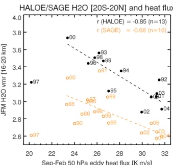
Fig. 2. Anti-correlation between JFM TLS water vapor VMRs
(16–20 km, 20◦S–20◦N) from SAGE II (open orange circles) and HALOE (filled black circles) and 50 hPa eddy heat flux added from both hemispheres and averaged over the period September-February. The correlation coefficients as indicated in the plot have been derived by excluding the year 1997 (see main text for discus-sions). The two digit indicate the year, for instance, 97 indicates 1996/97.
Yamazaki, 1999). Ascending motion in TLS is maximum during northern hemisphere winter which can be explained by a superposition of wave activity (or eddy heat flux) from both hemispheres (Rosenlof and Holton, 1993; Randel et al., 2002a; Salby et al., 2003). The maximum of the eddy heat flux is observed from November to March during NH win-ter and in the southern hemisphere (SH) from September to November, so that the total flux from both hemispheres shows large values from September to March (Randel et al., 2002a). This produces a seasonal variation in TLS tempera-tures (Yulaeva et al., 1994; Randel et al., 2002b) and, hence together with vertical advection explains the so-called tape recorder effect in tropical stratospheric water vapor with low (high) WV when tropical stratospheric temperatures are min-imum (maxmin-imum) during the seasonal cycle (Mote et al., 1996).
In Fig. 1, we selected mean water vapor profiles averaged between 16 and 20 km in order to reduce the large uncer-tainties associated with the solar occultation data closer to the lowest retrieval altitudes. The speed of upward propaga-tion of the WV anomalies is generally about 8 km/year (up-per limit derived from a tape recorder plot, not shown here) or 6 km/year assuming a mean ascent velocity of 0.2 mm/s (Randel et al., 2006, Fig. 9), so that the vertical averaging leads to some smearing of the tape recorder signal. Since water vapor is quite a good tracer (above the cold point), the
mean water vapor in the range 16–20 km, therefore, repre-sents roughly the cumulative amount of air transported into the stratosphere from the previous half year. Therefore, the observed water vapor minima as shown in Fig. 1 are shifted towards March–April. The strong inter-annual variability in mid-latitude wave driving, here represented by the aver-age eddy heat flux between 45◦–75◦ at 50 hPa and added from both hemispheres, is shown in Fig. 1. The color cod-ing indicates years with high wave activity (yellow-red) and low wave activity (violet-blue lines), when TLS water va-por VMRs are generally lower and higher, respectively. This is more emphasize in the scatter plot (Fig. 2) of tropical JFM water vapor VMRs and 50 hPa eddy heat flux integrated from September to February that shows a distinct anti-correlation between both quantities. Figure 2 shows average water va-por VMRs from HALOE (black solid symbols) and SAGE II (orange light symbols).
After filtering out the aerosol contaminated data (see Sect. 2) from SAGE II data, 17 years of SAGE II data since 1984 and 14 years of HALOE data (1992–2005) remained in this analysis. Lower stratospheric water vapor VMRs from SAGE II are systematically lower than HALOE in agree-ment with Taha et al. (2004). For all HALOE years the cor-relation between JFM ELS water vapor VMRs between 16 and 20 km and eddy heat flux is about −0.61 and excluding data from 1997 (here standing for 1996/1997), it improves to −0.85 (significant above 99% confidence interval). For SAGE II the correlation changes from −0.42 (including all years) to −0.68 after excluding 1997. Additionly removing the year 1991, the anti-correlation for SAGE II improves to
−0.77 (significant above 99% confidence level). As expected
higher global wave activity in a given year leads to lower wa-ter vapor VMRs in the tropical stratosphere at the end of the NH winter for most years. The period September-February for eddy heat flux and January–March for water vapor were selected for the highest anti-correlation between both quan-tities. The length of the September–February period roughly corresponds to the water vapor cumulation time in the 16– 20 km column based upon typical ascent velocities discussed before. It should be kept in mind that the near global sam-pling of the solar occultation instruments like SAGE II and HALOE requires more than a month. This leads to rather low sampling of the tropical stratosphere when zonal monthly means are derived and this may (in part) influence the cor-relation between both data sets.
We also find that by using eddy heat flux only from the NH the correlation coefficient is about −0.73 for HALOE data (without 1997) but for SAGE II data, it reduces sig-nificantly to −0.4 even without the years 1990/1991 and 1996/1997. Using eddy heat flux at 100 hPa or 70 hPa also re-duces the correlation coefficients. A possible explanation for the higher correlation with the 50 hPa eddy heat fluxes lies in differences in the mid-latitude wave driving between both hemispheres. The stationary planetary waves (wavenumber 1–3) and transient synoptic scale waves (wavenumber 4–7)
S. Dhomse et al.: BD circulation and water vapor 475 play an important role in driving the BD circulation in the
NH while in the SH most of the contribution comes from the transient waves (Tanaka et al., 2004). However, the contribu-tion from higher wave number waves to the total eddy heat flux at 100 hPa is quite small.
For some years like 1990/91 (91 in Fig. 2) and 1996/97 (97 in Fig. 2) larger deviations from the linear relationship be-tween extratropical wave driving and water vapor are notice-able. The year 1997 shows very low TLS water vapor VMRs (both SAGE II and HALOE measurements), despite the fact that the winter eddy heat flux is quite low. The opposite is true for 1990/91 (SAGE II only), where both the cumulative eddy heat flux and water vapor VMRs are high. An expla-nation for the extreme departure from the linear relationship for both satellite data is not known. The increase in water vapor at the TTL have been related to El Ni˜no events (Get-telman et al., 2002; Hatsushika and Yamazaki, 2000; Scaife et al., 2003). In early 1997 the Southern Oscillation Index (SOI) shows very low values indicating the beginning of a strong El Ni˜no event, however, in JFM of 1998 the TLS wa-ter vapor VMRs appears to be normal, although the Southern Oscillation Index (SOI) remained very low. Such exceptions highlight that the expected relationship between the BD cir-culation strength and tropical stratospheric water vapor does not hold for all years. Cold point temperature modeled wa-ter vapor VMRs (see Fig. 2 from F¨uglistaler and Haynes, 2005) are in agreement with HALOE and SAGE II in 1997, however, they differ significantly for years 1990 and 1993 (due to Mount Pinatubo eruption) from observations. Randel et al. (2004b) also noted that even though tropical cold point temperatures show a strong correlation with observed water vapor VMRs at 82 hPa, the years 1997/98, 1999/2000, and 2001/2002 show some unusual behavior (see Fig. 13 from Randel et al., 2004b).
Some studies argue that the tropical upwelling is not only driven by extratropical wave driving, but may be linked to the non-linear interaction between various physical processes in the tropical atmosphere such as equatorial Rossby waves and associated adiabatic heating (Plumb and Eluszkiewicz, 1999; Semeniuk and Shepherd, 2001). Temperatures in the tropical tropopause layer (TTL) that control the water vapor entry into the stratosphere can also be associated with tro-pospheric processes related to convection and tropical waves (Kerr-Munslow and Norton, 2006; Norton, 2006). Another issue here is the rather low sampling rate of solar occultation instruments as discussed before, however, it can not explain the obvious outliers in the expected relationship between ex-tratropical wave forcing and stratospheric water vapor in se-lected years as observed in the both satellite instrument data sets.
Fig. 3. Top panel: monthly mean H2O vapor anomalies from
HALOE (16–20 km, 20◦S–20◦N) in the tropics (black line) and POAM III (14–18 km) at middle to high NH latitudes (red line). Both lines represent three month mean water vapor VMRs, while black circles are monthly mean HALOE values (Update from Ran-del et al., 2006). Bottom panel: Time series of monthly mean 50 hPa eddy heat flux anomalies in each hemisphere and globally (added from both hemispheres).
4 Decrease in TLS H2O vapor after 2000
As seen in Figs. 1 and 2 and reported in other studies (Ran-del et al., 2004b, 2006), lower water vapor VMRs have been observed in the TLS since 2001 indicating that the strato-sphere has become drier in recent years. Lower water vapor VMRs are also found in NH mid- to high latitudes with a time lag of a few months due to isentropic transport in the lower-most stratosphere as confirmed by POAM III data (Randel et al., 2006). Figure 3 shows the water vapor VMR anomaly time series from HALOE in the tropics and POAM III at NH mid- to high latitudes (Nedoluha et al., 2002) in the lower-most stratosphere. Anomalies are calculated by subtracting the long-term monthly means (1992–2005) from the time se-ries. Both data sets clearly show negative anomalies after 2000. Coinciding with the sudden drop in TLS water va-por, a sudden increase in the monthly mean eddy heat flux is evident as shown in Fig. 3. The enhancement in eddy heat flux is consistent with increased tropical upwelling veloci-ties during the same time period and average enhancement in the subtropical convergence of the EP fluxes during the pe-riod 2001–2004 in comparison with the late 1990s (Randel et al., 2006). From the eddy heat flux time series separated
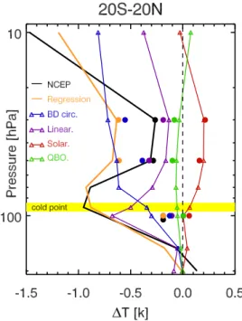
Fig. 4. Temperature anomalies of the zonal mean cold point
tem-perature from NCEP (20◦S–20◦N) and fitting results from a re-gression with contributions from QBO, monthly linear trends, solar variability, stratospheric aerosols, and BD circulation strength (as expressed by the extratropical 50 hPa eddy heat flux). Linear trends are only shown January and June. The strengthening of the BD cir-culation after 2000 resulted in a cooling of about 0.4 K at this level compared to the late 1990s (see horizontal bars in the BD circula-tion panel). The NCEP data shows a mean cooling of nearly 1 K after 2000 (horizontal bars in the bottom panel).
by hemispheres (Fig. 3) it can be concluded that each hemi-sphere contributed roughly equally (NH being slightly larger) to the eddy heat flux anomaly after 2000.
The increase in planetary wave driving in the NH in re-cent years has been associated with increased Arctic straspheric winter temperatures and rapid increases in NH to-tal ozone since the middle 1990s (Dhomse et al., 2006). An anti-correlation between tropical and mid- to high lati-tude lower stratospheric temperatures exists on seasonal and inter-annual time scales (Yulaeva et al., 1994; Salby and Callaghan, 2002) so that a corresponding recent cooling of the TLS and cold point temperature are expected. Figure 4 shows a time series of the tropical monthly mean temperature anomaly of the thermal tropopause from NCEP and a regres-sion analysis that quantifies the contributions from QBO, so-lar cycle variability, stratospheric aerosols, eddy heat flux, and linear trend terms. The linear trend terms account for changes that are not accounted for by other factors and terms. For each month of the year two QBO terms (50 and 30 hPa, 24 fitting constants), one eddy heat flux term (12 fitting stants, no time lag), and a linear trend term (12 fitting con-stants) are included. One fitting constant for each major vol-canic eruption and solar term are also included (for details on regression see Dhomse et al., 2006). The regression
anal-Fig. 5. Average tropical temperature profile change between the
pe-riods 7/2000–6/2005 and 7/1996–6/2000. Thick solid lines: NCEP re-analysis (black) and regression analysis (orange). Other lines with small symbols: individual contributions from solar activity, QBO, and linear trend as derived from 27 years of NCEP data. Large solid circle are the same results, but derived from the HadAT2 radio sonde data. The results for the mean cold point temperatures from NCEP are displayed at the approximate mean cold point alti-tude of 93 hPa.
ysis has been applied to several pressure levels (100, 70, 50, 30, and 10 hPa, and cold point altitude) as well to isobaric ERA40 data (up to August 2002) and HadAT2 data (100, 50, 30 hPa). The regression coefficients (for various terms) are similar for both NCEP and ERA40, but not for HadAT2 data, where long term linear trends are lower than either ERA40 and NCEP data. In general the eddy heat flux contribution to the temperature change is statistically significant (2σ ) from the cold point altitude up to 30 hPa. With radiative lifetime ranging from about 100 days (100 hPa) to 50 days at 50 to 30 hPa (Randel et al., 2002a; Niwano et al., 2003), the dia-batic warming relaxation after the adiadia-batic expansion from the extratropical wave driving is sufficiently slow to detect a temperature change with no time lag in the eddy heat flux. Our regression analysis indicates that the strengthening of the BD circulation contributed nearly 0.4 K cooling to the total changes in the zonal mean cold point temperature when com-paring a five year period before and after the drop in water vapor anomalies in 2000 (see the horizontal bars in the BD circulation contribution to the temperature trend in Fig. 4).
The change in the vertical tropical temperature profile from NCEP and HadAT2 and the 25 year regression ap-plied to both datasets between the period 7/2000–6/2005 and 7/1996–6/2000 is shown in Fig. 5. From the NCEP data an
S. Dhomse et al.: BD circulation and water vapor 477 overall temperature change after 2000 is evident at 100 hPa
(−0.8 K), cold point altitude (−0.9 K), and 70 hPa (−1.0 K), while at 50 hPa and 30 hPa the total temperature change is smaller. The increase in wave driving (or the strength of BD circulation) after 2000 may have contributed a cooling of 0.2 K at 100 hPa, nearly 0.4 K at the cold point altitude, and 0.7 K at 50 hPa and 30 hPa to the NCEP temperatures, com-pared to a range of 0.1 K (100 hPa) to 0.7 K (30 hPa) to the HadAT2 radio sonde data. The regression analyses tend to overestimate the overall cooling (including all contributions) above 70 hPa. A stronger cooling in the TLS compared to the cold point temperature would require enhanced adiabatic expansion and upwelling velocities increasing with altitude. According to Fig. 4 in Niwano et al. (2003) an increasing upwelling velocity with altitude is observed in the HALOE methane and water vapor data.
As mentioned earlier, F¨uglistaler and Haynes (2005) found that a 1 K cooling in the cold point temperature roughly cor-responds to a decrease of 0.5 ppm in TLS water vapor. This is consistent with cold point temperature changes from extra-tropical wave forcing of about −0.4 K and an average water vapor decrease of 0.2 to 0.3 ppm after 2000 (see Fig. 3). The contribution from the extratropical wave forcing to 100 hPa temperature is rather small, which is an indication that the 100 hPa level is mostly well inside the TTL layer, where the stratospheric influence becomes negligible. In contrast to NCEP data HadAT2 radiosonde data shows almost no changes in 100 hPa temperatures between the five year peri-ods before and after 2000; the cooling seen in the NCEP data primarily has its main contribution from an apparent decadal linear trend that is absent in the radio sonde data. There is some considerable debate on the significance of these lin-ear trends nlin-ear the tropical tropopause, since changes in ra-diosonde operations (cooling bias) and changes in the assim-ilation scheme may strongly impact such long-term trends particularly near the tropical tropopause (see discussion in Randel et al., 2004b, 2006, and references therein).
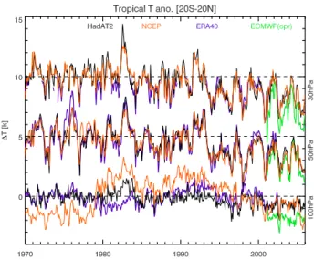
The larger uncertainties associated with the temperature data sets are more evident when looking at different meteoro-logical analyses that are currently avaliable. Figure 6 shows temperature anomalies in the TLS derived from various anal-yses, ERA40 (1958–2002), ECMWF operational analysis data set (2001–present), NCEP (1948–present), and the Ha-dAT2 radiosonde data set. Shown are monthly mean tem-perature anomalies over the tropics (20◦S–20◦N) at 100 hPa (bottom), 50 hPa (middle) and 30 hPa (top). Anomalies were calculated by subtracting the climatological monthly means over the period 1965–1995 period from the timeseries. At 50 hPa and 30 hPa no significant bias in the NCEP data is noticeable with respect to the homogenized radiosonde data especially after NCEP switched from TOVS to ATOVS data (Randel et al., 2004b) in July 2001. The ERA40 reanalysis from ECMWF that ended in 2002 shows a bias with respect to the ECMWF operational analysis that ranges from +1 K to +2 K at all altitudes during the overlapping period (January
Fig. 6. Temperature anomalies in the TLS (20◦S–20◦N) from different meteorological analyses. Temperature anomalies from ERA40 (Uppala et al., 2005) are shown in blue and from ECMWF operational data in green. NCEP (Kalnay et al., 1996) and HadAT2 (Thorne et al., 2005) are shown in orange and black, respectively. Monthly mean anomalies are calculated by subtracting the long-term monthly means (1965–1995) from the time series. Temper-ature anomalies at 50 hPa and 30 hPa are shifted by 5 K and 10 K respectively, for clarity. The temperature anomalies from ECMWF operational data show a cold bias (1–2 K) with respect to ERA40.
2001–August 2002). This is an indication of uncertainties in temperatures from differences in the assimilation schemes.
There are significant differences among these analyses at 100 hPa. The NCEP data show a larger linear cooling trend after the middle 1990s than either the radio sonde data or ERA40 as discussed before, nevertheless a jump of about of about −0.5 to −1 K during 2000 is noticeable in all data sets (this difference nearly vanishes when averaging over five year periods before and after 2000). The temperature vari-ability apart from spurious linear trends is strongly reduced at 100 hPa (below ±1 K), which is an indication of a weaken-ing of the stratospheric influence as one goes deeper into the TTL region, while the higher altitudes (above and including the cold point temperature altitude) show larger variations in the anomalies mainly influenced by the QBO and extratrop-ical wave-driving as shown as an example in Fig. 5. The NH winter 1996/1997 that was regarded as an outlier in the TLS water vapor – eddy heat flux anti-correlation (marked 1997 in Fig. 2) shows good agreement in the regression anal-ysis of TLS temperatures (positive anomalies in eddy heat flux and temperatures, while at 100 hPa and cold point al-titude the negative temperature anomaly (Fig. 4) appears to be more consistent with observations of low water vapor ob-servations in that year. One year later (1997/98) the mod-eled temperature at 70 hPa and 50 hPa are higher than the ob-served temperature, which makes the five year period before 2000 warmer and the difference to the late period as shown in Fig. 5 larger (more cooling) in the regression.
While the cooling contribution from enhanced eddy heat flux to the NCEP cold point temperature (−0.4 K) after 2000 agree quite well with the observed water vapor change, the total temperature change of nearly −1 K should have doubled the reduction in water vapor in the lowermost tropical strato-sphere. The observed long-term downward trends apart from the sudden jump during 2000 is not evident in the water va-por observations. As the homogenized HadAT2 radio sonde data show in contrast to NCEP no linear trend at 100 hPa, it is very likely that the spurious long-term trends are rather artefacts from the larger uncertainties in the radio sonde data that are assimilated into the meteorological analysis.
5 Conclusions
We have shown that satellite data from HALOE and SAGE II show inter-annual variability in TLS water vapor that is anti-correlated with the mid-latitude wave driving (or the strength of the BD circulation) with an exception of few years, i.e. 1990/1991, 1996/1997 (Fig. 2). The departure in some years point out that WV variability in TLS can not be attributed solely to changes in extratropical wave driving, although the agreement between changes in tropical cold point tempera-ture (F¨uglistaler et al., 2005) as well as tropical upwelling (Randel et al., 2004b, 2006) and water vapor changes are generally good also in these years. Some studies argue that the tropical upwelling may be also linked to the non-linear interaction between various physical processes in the tropi-cal atmosphere such as equatorial Rossby waves, other trop-ical waves, and convection (Plumb and Eluszkiewicz, 1999; Semeniuk and Shepherd, 2001; Kerr-Munslow and Norton, 2006; Norton, 2006).
The sudden decrease of about 0.2 ppm in the lower strato-spheric water vapor after 2000 that has persisted until 2005 can be directly related to an enhanced wave driving with nearly equal forcing from extratropical wave driving in each hemisphere (Fig. 3). F¨uglistaler and Haynes (2005) argued that variations in ELS water vapor and cold point tempera-tures are mainly influenced by the QBO and ENSO (El Nino-Southern oscillation). The QBO and extratropical wave driv-ing are to some extent coupled with each other through the Holton-Tan mechanism (Holton and Tan, 1980). Since the water vapor anomalies must be related to dehydration mech-anism in the TTL, the signature from extratropical wave driv-ing on tropical temperatures have been analyzed by a regres-sion analysis including contributions from QBO, solar cy-cle, 50 hPa middle latitude eddy heat flux, and linear trend terms, the latter accounting for all other possible contribu-tions (Fig. 4).
In connection with the enhanced extratropical wave forc-ing nearly 0.7 K coolforc-ing was estimated at 70 hPa and above. However, combining the contribution from all the relevant processes, our regression model overestimates the cooling above 70 hPa (Fig. 5). The cold point temperature derived
from the NCEP data shows a cooling of 1.0 K after 2000 compared to the late 1990s, however, only a fraction of 0.4 K are associated with the increased wave activity. The latter cooling contribution is consistent with an decrease of −0.2 to −0.3 ppm in the observed water vapor (Fig. 3). An ap-parent long-term downward trend in the NCEP cold point temperature contributes largely to the overall cooling, that appears to be absent in the HadAT2 data at 100 hPa. This is an indication that there may be large uncertainties associated with the temperature data near the TTL (Randel et al., 2004b, 2006). On the other hand, the observed reduction of 10% in ozone near the TTL from the late 1990s to early 2000s may reduce temperatures by −0.5 K via radiative feedbacks (Ran-del et al., 2006) and could contribute to such a linear trend, however, a corresponding enhanced trend in the water vapor is not evident. The HadAT2 data show very little interannual variability at 100 hPa, which suggests that this pressure level for most part of the annual cycle is likely inside the TTL, where the stratospheric influence diminishes.
Exact causes of the recent enhanced extratropical wave driving are not clear but if this pattern persists, it will sig-nificantly alter the lifetime of most of the chemical species in the stratosphere. A coherent picture of changes in mid-to high latitude ozone (Dhomse et al., 2006) and lower stratospheric water vapor in connection with BD circulation changes emerges that may have important implications in a future changing climate.
Acknowledgements. This study is supported by EU project SCOUT
and DFG project SOLOZON. We thank the NASA teams for pro-viding SAGE and HALOE data sets and NRL for POAM data. The support of NCEP, ECMWF and UK Met. Office for providing the meteorological analysis is gratefully acknowledged. ECMWF data were made available thru the ECMWF Special project SPDECDIO. We thank P. Haynes, B. Randel, B. M. Sinnhuber, S. F¨ueglisthaler and three anonymous referees for helpful comments to different versions of the manuscript.
Edited by: P. Haynes
References
Brewer, A. W.: Evidence for a world circulation provided by the measurements of helium and water vapour distribution in the stratosphere, Q. J. R. Meteorol. Soc., 75, 351–363, 1949. Dhomse, S., Weber, M., Burrows, J., Wohltmann, I., and Rex, M.:
On the possible causes of recent increases in NH total ozone from a statistical analysis of satellite data from 1979 to 2003, Atmos. Chem. Phys., 6, 1165–1180, 2006,
http://www.atmos-chem-phys.net/6/1165/2006/.
F¨uglistaler, S. and Haynes, P.: Control of interannual and longer-term variability of stratospheric water vapor, J. Geophys. Res., 110, D24108, doi:10.1029/2005JD006019, 2005.
F¨uglistaler, S., Bonazzola, M., Haynes, P., and Peter, T.: Strato-spheric water vapor predicted from the Lagrangian temperature history of air entering the stratosphere in the tropics, J. Geophys. Res., 110, D08107, doi:10.1029/2004JD005516, 2005.
S. Dhomse et al.: BD circulation and water vapor 479
Fusco, A. C. and Salby, M. L.: Interannual variations of total ozone and their relationship to variations of planetary wave activity, J. Climate, 12, 1619–1629, 1999.
Gettelman, A., Randel, W. J., Wu, F., and Massie, S. T.: Transport of water vapor in the tropical tropopause layer, Geophys. Res. Lett., 29(01), 1009, doi:10.1029/2001GL013818, 2002. Hatsushika, H. and Yamazaki, K.: Interannual variations of
temper-ature and vertical motion at the tropical tropopause associated with ENSO, Geophys. Res. Lett., 28(15), 2891–2894, 2000. Haynes, P. H., Marks, C. J., McIntyre, M. E., Shepherd, T. G., and
Shine, K. P.: On the “downward control” of extratropical diabatic circulations by eddy-induced mean zonal forces, J. Atmos. Sci., 48, 651–678, 1991.
Holton, J. and Tan, H.-C.: The influence of the equatorial quasi-biennial oscillation on the global circulation at 50 mb, J. Atmos. Sci., 37, 2200–2208, 1980.
Kalnay, E., Kanamitsu, M., Kistler, R., Collins, W., Deaven, D., Gandin, L., Iredell, M., Saha, S., White, G., Woolen, J., Zhu, Y., Chelliah, M., Ebisuzaki, W., Higgins, W., Janowiak, J., Mo, K. C., Ropelewski, C., Wang, J., Leetma, A., Reynolds, R., Jenne, R., and Joseph, D.: The NCEP/NCAR 40-year reanaly-sis project, Bullet. Amer. Meteorol. Soc., 77, 437–471, 1996. Kerr-Munslow, A. M. and Norton, W. A.: Tropical wave driving
of the annual cycle in tropical tropopause temperatures Part I: EMCWF analyses, J. Atmos. Sci., 63(5), 1410–1419, 2006. Mote, P., Rosenlof, K. H., Holton, J. R., Harwood, R. S., and
Wa-ters, J. W.: An atmospheric tape recorder: The imprint of tropical tropopause temperatures on stratospheric warter vapor, J. Geo-phys. Res., 101, 3989–4006, 1996.
Nedoluha, G. E., Bevilacqua, R. M., Hoppel, K. W., Lumpe, J. D., and Smith, H.: Polar Ozone and Aerosol Measurement III measurements of water vapor in the upper troposphere and lower stratosphere, J. Geophys. Res., 108, 4391, doi:10.1029/ 2002JD003332, 2002.
Newman, P. A., Nash, E., and Rosenfield, J.: What controls the temperature of the Arctic stratosphere during the spring?, J. Geo-phys. Res., 106, 19 999–20 010, 2001.
Niwano, M., Yamazaki, K., and Shiotani, M.: Seasonal and QBO variations of ascent rate in the tropical lower stratosphere as in-ferred from UARS HALOE trace gas data, J. Geophys. Res., 108(D24), 4794, doi:10.1029/2003JD003871, 2003.
Norton, W. A.: Tropical wave driving of the annual cycle in tropical tropopause temperatures, Part II: Model results, J. Atmos. Sci., 63(5), 1420–1431, 2006.
Oltmans, S. J., Voemel, H., Hofmann, D. J., Rosenlof, K. H., and Kley, D.: The increase in stratospheric water vapor from bal-loonborne, frostpoint hygrometer measurements at Washington, D.C., and Boulder, Colorado, Geophys. Res. Lett., 27(21), 3453– 3456, 2000.
Plumb, A. R. and Eluszkiewicz, J.: The Brewer-Dobson circulation: Dynamics of the tropical upwelling, J. Atmos. Sci., 56(6), 868– 890, 1999.
Randel, W., Udelhofen, P., Fleming, E., Geller, M., Gelman, M., Hamilton, K., Karoly, D., Ortland, D., Pawson, S., Swinbank, R., Wu, F., Baldwin, M., Chanin, M., Keckhut, P., Labitzke, K., Remsberg, E., Simmons, A., and Wu, D.: The SPARC inter-comparison of middle atmosphere climatologies, J. Climate, 17, 986–1003, 2004a.
Randel, W. J., Garcia, R. R., and Wu, F.: Time dependent upwelling
in the tropical lower stratosphere estimated from the zonal-mean momentum budget, J. Atmos. Sci., 59, 2141–2152, 2002a. Randel, W. J., Wu, F., and Stolarski, R. S.: Changes in column
ozone correlated with the stratospheric EP flux, J. Meteor. Soc. Jpn., 80, 849–862, 2002b.
Randel, W. J., Wu, F., Oltmans, S. J., Rosenlof, K., and Nedoluha, G. E.: Interannual changes of stratospheric water vapor and cor-relations with tropical tropopause temperatures, J. Atmos. Sci., 61, 2133–2148, 2004b.
Randel, W. J., Wu, F., Voemel, H., Nedoluha, G. E., and Forster, P.: Decreases in stratospheric water vapor after 2001: links to changes in the tropical tropopause and the Brewer-Dobson circulation, J. Geophys. Res., 111, 12 312, doi:10.1029/ 2005JD006744, 2006.
Rosenlof, K.: How water enters the stratosphere, Science, 302, 1691–1692, 2003.
Rosenlof, K. and Holton, J. R.: Estimates of the stratospheric resid-ual circulation using the downward control principle, J. Geophys. Res., 98, 10 465–10 479, 1993.
Russell, J. M., Gordley, L. L., Park, J. H., Drayson, S. R., Hesketh, D. H., Cicerone, R. J., Tuck, A. F., Frederick, J. E., Harries, J. E., and Crutzen, P. J.: The Halogen Occultation Experiment, J. Geophys. Res., 98(D6), 10 777–10 797, 1993.
Salby, M., Sassi, F., Callaghan, P., Read, W., and Pumphrey, H.: Fluctuations of cloud, humidity and thermal structure near tropi-cal tropopause, J. Climate, 16, 3428–3446, 2003.
Salby, M. L. and Callaghan, P. F.: Interannual changes of the stratospheric circulation: Relationship to ozone and tropospheric structure, J. Climate, 15, 3673–3685, 2002.
Scaife, A. A., Buchart, N., Jackson, D. R., and Swinbank, R.: Can changes in ENSO activity help to explain increasing strato-spheric water vapor?, Geophys. Res. Lett., 30, 1880, doi:10. 1029/2003GL017591, 2003.
Semeniuk, K. and Shepherd, T. G.: Mechanisms for tropical up-welling in the stratosphere, J. Atmos. Sci., 58(21), 3097–3115, 2001.
Seol, D. and Yamazaki, K.: Residual mean meridional circulation in the stratosphere and upper troposphere: Climatological aspects, J. Meteor. Soc. Jpn., 77(5), 985–996, 1999.
Shindell, D. T.: Climate and ozone response to increased strato-spheric water vapor, Geophys. Res. Lett., 28, 1551, doi:10.1029/ 1999GL011197, 2001.
Shindell, D. T., Miller, R. L., Schmidt, G. A., and Pandolfo, L.: Simulation of recent northern winter climate trends by greenhouse-gas forcing, Nature, 399, 452–455, 1999.
SPARC: Assesment of upper tropospheric and stratospheric water vapour, chap. Conclusions, World Climate Research Programme, WCRP-113,WMO/TD-No.1043, 261–264, 2000.
Stenke, A. and Grewe, V.: Simulation of stratospheric water vapor trends: Impact on stratospheric ozone chemistry, Atmos. Chem. Phys., 5, 1257–1272, 2005,
http://www.atmos-chem-phys.net/5/1257/2005/.
Tabazadeh, A., Santee, M. L., Danilin, M. Y., Pumphrey, H. C., Newman, P. A., Hamill, P. J., and Mergenthaler, J. L.: Quantify-ing denitrification and its Effect on ozone recovery, Science, 288, 1407–1411, 2000.
Taha, G., Thomason, L. W., and Burton, S. P.: Comparison of Stratospheric Aerosol and Gas Experiment (SAGE II) version 6.2 water vapor with balloon-borne and space-based instruments,
J. Geophys. Res., 109, D18313, doi:310.1029/2004JD004859, 2004.
Tanaka, D., Iwasaki, T., Uno, S., Ujiie, M., and Miyazaki, K.: Eliassen Palm flux diagnosis based on isentropic representation., J. Atmos. Sci., 61, 2370–2383, 2004.
Thomason, L. W., Burton, S. P., Iyer, N., Zawodny, J. M., and An-derson, J.: A revised water vapor product for the Stratospheric Aerosol and Gas Experiment (SAGE) II version 6.2 data set, J. Geophys. Res., 109, D06312, doi:10.1029/2003JD004465, 2004. Thorne, P. W., Parker, D. E., Tett, S., Jones, P. D., McCarthy, M., Coleman, H., and Brohan, P.: Revisiting radiosonde upper air temperatures from 1958 to 2002, J. Geophys. Res., 110, D18105, doi:10.1029/2004JD005753, 2005.
Uppala, S. M., K¨allberg, P. W., Simmons, A. J., Andrae1, U., da Costa Bechtold, V., Fiorino, M., Gibson, J. K., Haseler, J., Hernandez, A., Kelly, G. A., Li, X., Onogi, K., Saarinen, S., Sokka, N., Allan, R. P., Andersson, E., Arpe, K., Balmaseda, M. A., Beljaars, A. C. M., van de Berg, L., Bidlot, J., Bormann, N., Caires, S., Chevallier, F., Dethof, A., Dragosavac, M., Fisher, M., Fuentes, M., Hagemann, S., Holm, E., Hoskins, B. J., Isak-sen, L., JansIsak-sen, P. A. E. M., Jenne, R., McNally, A. P., Mahfouf, J., Morcrette, J., Rayner, N. A., Saunders, R. W., Simon, P., Sterl, A., Trenberth, K. E., Untch, A., Vasiljevic, D., Viterbo, P., and Woollen, J.: The ERA40 analysis, Q. J. Roy. Meteor. Soc., 131, 2961–3012, doi:10.1256/qj.04.176, 2005.
Weber, M., Dhomse, S., Wittrock, F., Richter, A., Sinnhuber, B., and Burrows, J.: Dynamical control of NH and SH winter/spring total ozone from GOME observations in 1995-2002, Geophys. Res. Lett., 30, 1853, doi:10.1029/2002GL016799, 2003. Yulaeva, E., Holton, J. R., and Wallace, J. M.: On the cause of the
annual cycle in the tropical lower stratospheric temperature, J. Atmos. Sci., 51, 169–174, 1994.