Comparison of gliding box and box-counting methods in river network analysis
Texte intégral
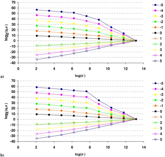
Figure

Documents relatifs
(We will not use this equation in this elementary talk: it holds in the distribution sense , for N > 1, because of C N−2 -differentiability properties)... This property follows
To be able to predict the proper size and locations of per- sons and meanwhile bypass the need for expensive bound- ing box annotations, we introduce a new deep detection net-
Slap Tongue: Produced by puffing short tones with tongue to create a
Le vortex qu’est la boîte jouerait alors comme une camera oscura, une chambre obscure retournant la réalité en une image inversée, idéalisée : dans son rêve, Diane,
We present the numerical analysis on the Poisson problem of two mixed Petrov-Galerkin finite volume schemes for équations in divergence form div c/?(ti, Vit) = ƒ.. The first
Wordpress – Aller plus loin Personnaliser les thèmes. Personnaliser
This paper points out the issue of drawing meaningful relations between what is individually learned by the different subsystems of integrated systems and, furthermore, questions
Typical results of the prediction efficiency of Angular software failures using Holt – Winters and ARIMA models are listed in Table 1.. While the performance of ARIMA model is
