On the fast response of the Southern Ocean to changes in the zonal wind

(1)

HAL Id: hal-00298387

https://hal.archives-ouvertes.fr/hal-00298387

Submitted on 14 Jun 2006

HAL is a multi-disciplinary open access

archive for the deposit and dissemination of sci-entific research documents, whether they are pub-lished or not. The documents may come from teaching and research institutions in France or abroad, or from public or private research centers.

L’archive ouverte pluridisciplinaire HAL, est destinée au dépôt et à la diffusion de documents scientifiques de niveau recherche, publiés ou non, émanant des établissements d’enseignement et de recherche français ou étrangers, des laboratoires publics ou privés.

On the fast response of the Southern Ocean to changes

in the zonal wind

D. J. Webb, B. A. de Cuevas

To cite this version:

D. J. Webb, B. A. de Cuevas. On the fast response of the Southern Ocean to changes in the zonal wind. Ocean Science Discussions, European Geosciences Union, 2006, 3 (3), pp.471-501. �hal-00298387�

(2)

OSD

3, 471–501, 2006

The fast response of the Southern Ocean

D. J. Webb and B. A. de Cuevas Title Page Abstract Introduction Conclusions References Tables Figures J I J I Back Close Full Screen / Esc

Printer-friendly Version Interactive Discussion

EGU

Ocean Sci. Discuss., 3, 471–501, 2006 www.ocean-sci-discuss.net/3/471/2006/ © Author(s) 2006. This work is licensed under a Creative Commons License.

Ocean Science Discussions

Papers published in Ocean Science Discussions are under open-access review for the journal Ocean Science

On the fast response of the Southern

Ocean to changes in the zonal wind

D. J. Webb and B. A. de Cuevas

National Oceanography Centre, Southampton SO14 3ZH, UK

Received: 20 April 2006 – Accepted: 28 April 2006 – Published: 14 June 2006 Correspondence to: D. J. Webb (david.webb@noc.soton.ac.uk)

(3)

OSD

3, 471–501, 2006

Abstract

Model studies of the Southern Ocean, reported here, show that the Antarctic Circum-polar Current responds within two days to changes in the zonal wind stress at the latitudes of Drake Passage. Further investigation shows that the response is primarily barotropic and that, as one might expect, it is controlled by topography. Analysis of

5

the results show that the changes in the barotropic flow are sufficient to transfer the changed surface wind stress to the underlying topography and that during this initial phase baroclinic processes are not involved.

The model results also show that the Deacon Cell responds to changes in the wind stress on the same rapid time scale. It is shown that the changes in the Deacon

10

Cell can also be explained by the change in the barotropic velocity field, an increase in the zonal wind stress producing an increased northward flow in shallow regions and southward flow where the ocean is deep. This new explanation is unexpected as previously the Deacon Cell has been thought of as a baroclinic feature of the ocean.

The results imply that where baroclinic processes do appear to be involved in either

15

the zonal momentum balance of the Southern Ocean or the formation of the Deacon Cell, they are part of the long term baroclinic response of the ocean’s density field to the changes in the barotropic flow.

1 Introduction

The paper by Munk and Palm ´en (1951) was one of the first to raise the problem of

20

the zonal momentum balance in the Southern Ocean. At most latitudes the stress exerted on the ocean by zonal winds can be balanced by pressure differences between the eastern and western boundaries of the ocean. However at the latitudes of Drake Passage there are no such boundaries and so an alternative mechanism has to be found.

25

(4)

OSD

3, 471–501, 2006

EGU

transferred to the surface layers of the ocean, causing a northward Ekman transport. The stress was then transferred to topography when the flow returned southwards below the level of the Drake Passage sill. Later model studies supported this theory.

Stevens and Ivchenko(1996) in an analysis of the FRAM (1991) model showed that the surface Ekman layer almost exactly balanced the wind stress and that there was a

5

return flow at depth which transfered an almost equal amount of stress to the abyssal topography. Webb (1993) proposed a simple theory which showed how such a flow could generate an Antarctic Circumpolar Current with a realistic total transport.

Alternative theories have tended to involve the baroclinic circulation of the ocean.

Johnson and Bryden(1989) argued that the surface wind stress could be transferred

10

downward by baroclinic eddies and provided evidence that the strength of the eddy field in the Southern Ocean was sufficient to do this. Marshall et al. (1993), Gille

(1995) andIvchenko et al.(1969) all considered the momentum balance following the mean streamlines of the Antarctic Circumpolar Current and argued that any balance must involve baroclinic eddy processes. These and other approaches are discussed

15

further in the WOCE review paper byRintoul et al.(2001).

A related problem is concerned with the Southern Ocean Deacon Cell. When the ocean currents are averaged zonally to produce a meridional overturning streamfunc-tion, the Deacon Cell shows up as a region of apparent downwelling near 40◦S, with associated upwelling near the latitudes of Drake Passage. The two regions are

con-20

nected by the Ekman layer at the surface and a deep return flow at depths between two and three thousand metres. This return flow is below the depth of the major sills, so given that the Ekman layer is also involved, it seems probable that the feature is connected to the momentum balance problem.

However although water may be upwelled from depth at the latitudes of Drake

Pas-25

sage, where the stratification is weak, it is not clear how downwelling occurs near 40◦S, where stratification is much stronger. The problem was investigated by D ¨o ¨os

and Webb (1994), who showed that the cell was associated with a large scale me-ander of the Antarctic Circumpolar Current (ACC). In the South Atlantic Sector, water

(5)

OSD

3, 471–501, 2006

Printer-friendly Version Interactive Discussion in the meander moved northwards at a slightly shallower depth than normal. It then

returned southwards, at a slightly deeper depth, in the remainder of its path around the Southern Ocean. In the centre of the cell at mid-depths, the northward and southward flow of water of different densities cancel out so the streamfunction remains constant. However in the surface Ekman layer and at depth, (and also when considering vertical

5

flow at the northern and southern limits of the cell), this cancellation does not happen and the streamfunction indicates a net transport.

The result of this work has been an emphasis on the importance of stratification and baroclinicity on the dynamics of the Southern Ocean. A number of the momentum balance theories involve baroclinic processes and even if one prefers the approach of

10

Munk and Palm ´en(1951), this explanation of the Deacon Cell indicates that stratifica-tion has a key role in the downward transfer of momentum from the wind.

However baroclinic processes cannot be responsible for everything. Hughes et al.

(1999) used model results to show that at periods between 10 and 220 days the ACC transport was dominated by a barotropic mode. Hughes et al.(2003) followed this up

15

using sea level data from Antarctica and the neighbouring oceans. The observations show rapid changes in the pressure gradient across Drake Passage, implying rapid changes in ACC transport. They showed that the changes are highly correlated with sea level measurements all around Antarctica and that they are only weakly correlated with sea level at islands far offshore (including islands south of the main ACC). They

20

find that the time taken for the signal to travel around Antarctica is a few days at most. The fast timescale implies that what they are seeing is a barotropic response of the ocean. The speed of barotropic waves is fast; the tides with speeds of order 200 ms−1 are able to circle Antarctica in a day or so. In contrast baroclinic waves have speeds of 2 ms−1 or less and so would take a hundred times longer to propagate around the

25

continent.

The spur for the present investigation came partly from these fast response results and partly from an observation made during the spin-up phase of the FRAM model, when the ACC transport was found to respond within five days to any changes in the

(6)

OSD

3, 471–501, 2006

EGU

applied wind stress field. To see if there was any connection, we set up a perturbation experiment using a global ocean model, and investigated the ocean’s response to a small rapid change in the zonal wind stress at the latitudes of Drake Passage.

To simplify the analysis we decided to initialise the model with a constant wind stress and with constant surface forcing. The model is initially spun up for ten model years,

5

so that when the perturbation in introduced at the end of this period, any changes are primarily due to the perturbation and not the residual response to any earlier events.

As we will see, the results confirm the work ofHughes et al. (1999), but show that even shorter timescales are involved. We find that the barotropic field alone is able to balance the surface wind stress at the latitudes of Drake Passage and it does this via

10

a mode which does not follow lines of f /h (where f is the Coriolis parameter and h is depth). Baroclinic processes may evetually become important, but the implication is that they are but a later response of the density field to the changed barotropic flow field.

2 Spin-up of the ocean model

15

The computer model chosen for this study was a 1◦ version of the OCCAM Global Ocean Model (Coward and de Cuevas,2005). The model is based on the Bryan-Cox-Semtner rigid lid ocean model (Bryan,1969;Semtner,1974;Cox,1984) but includes a free surface and other improvements, including Modified-Split-Quick advection for tracers in the horizontal (Webb et al.,1998) and an improved vertical advection scheme

20

for momentum (Webb, 1995)1. The model has 66 levels in the vertical, varying in thicknesses from 5 m at the surface to 208 m at a depth of 6470 m. The thickness of the bottom layer in each column is adjustable to give a better fit to topography. The latter was taken from a global ocean bathymetry dataset provided by Coward (private

1

These and other aspects of model design are discussed in the paper byGriffies et al.(2005) which describes the details of a similar global ocean model designed for climate studies.

(7)

OSD

3, 471–501, 2006

Printer-friendly Version Interactive Discussion communication).

The initial tracer fields (potential temperature and salinity) were interpolated from the WOCE SAC climatology (Gouretski and Jancke,1996) for all oceans except the Arctic. In the Arctic the fields were interpolated from theSteele et al.(2001) climatology. The initial velocities were set to zero. The model was then forced with the annual average

5

surface wind stress calculated from theSiefridt and Barnier (1993) climatology which is based on ECMWF analyses. A surface flux of heat and fresh water was imposed, designed to relax top model level (i.e. the top 5 m) to climatology with a timescale of 7.5 days2.

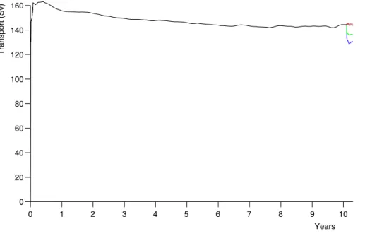
For the initial spin up the model was run for a period of ten model years. The ACC

10

transport through Drake Passage during this period is shown in Fig. 1. After an initial rapid rise to near 160 Sv3, the transport slowly declines to approximately 144 Sv at the end of the period. Over most of this period data was saved and is plotted at monthly intervals. The result shows that that the model has not reached a final steady state at the end of the period and that as well as a slow decline in transport there were some

15

oscillations with periods of less than a year. However this and similar figures showed no major features that may affect the rest of the analysis.

3 Changes in the wind stress

At the end of 3690 days (approximately 10 years and one month) the initial spin-up was stopped and the model fields archived. The archived data was then used for the initial

20

state in four short runs with different surface wind stresses.

In the first of these runs, the control, the wind stress was unchanged from the spin up phase. In Run 2, the perturbation run, the zonal wind stress was increased by 0.1 dyne

2

This was chosen to match earlier runs where the top 20 m had been relaxed with a timescale of 30 days.

3_{1 Sv=10}6

(8)

OSD

3, 471–501, 2006

EGU

cm−2at the latitudes of Drake Passage. A smoothing function F (θ) was used, where θ is latitude, defined so that the forcing tailed off linearly to north and south.

F (θ)= (70 − θ) if 70S ≥ θ > 64S = 1 if 64S ≥ θ > 55S = (θ − 49) if 55S ≥ θ > 49S

= 0 otherwise

Following the analysis of the perturbation run, two further runs were carried out involving larger changes in the wind field. In Run 3 the zonal wind stress was set to zero at the latitudes of Drake Passage. There should then be no northward Ekman transport at these latitudes and presumably no return flow at depth. The change was implemented, with smoothing as before, by multiplying the zonal wind by the function G(θ), where,

G(θ)= 1 − F (θ).

In the final run, Run 4, the zonal and meridional wind stresses were set to zero every-where.

4 Changes in the ACC transport

The ACC transports from the four short runs are shown in Fig. 1 and, on an expanded scale, in Fig. 2. The first result to notice is that the change in the transports is relatively

5

small. At day 2 the transport increases from 144.26 Sv in the control run to 144.96 Sv in the perturbation run, a change of 0.71 Sv. In the third, zero zonal wind stress run, the transport is 137.37 Sv, a reduction of 6.88 Sv, and in the fourth run, where the wind stress is set to zero everywhere, the transport drops to 136.09 Sv, a change of 8.16 Sv. The changes increase slightly with time, the differences at 30 days being 0.95 Sv for

(9)

OSD

3, 471–501, 2006

Printer-friendly Version Interactive Discussion the perturbation run, 7.95 Sv for the zero zonal wind and a much larger 15.06 Sv for

zero wind everywhere. The results are consistent with the observation made during the spin up of the FRAM model, when the addition of the wind stress increased the ACC transport by less than 20 Sv.

The second noticeable feature is that the ocean’s initial response to the changed

5

wind stress occurs very quickly. Even when the wind is turned off everywhere the bulk of the change in transport has occurred within 2.7 days. Given that the physical process must involve the generation of inertial oscillations, which die away leaving an Ekman layer, which then through other processes generates the change in the ACC transport, this is very fast indeed. It is comparable with the two to three day timescale

10

it takes for tidal waves to propagate throughout the ocean.

A third noticeable feature is that the zonal wind stress at the latitudes of Drake Pas-sage is only responsible for roughly half of the wind generated ACC transport. This is not unexpected because on theoretical grounds the steady state barotropic response of the ocean is likely to be associated with contours of f /h and these do not follow lines

15

of latitude. However only a fraction of the contours of f /h which pass through Drake Passage encircle the whole Southern Ocean so, in the absence of a full theory, their role remains unclear.

After the initial fast response to the change in wind stress, the transports also show some longer term oscillations. In Run 3, where the wind stress is set to zero at the

20

latitudes of Drake Passage, this shows up as an oscillation with a period of nine days which decays away after a month. There is also a longer period oscillation with a period of about two months. Setting the wind to zero everywhere produces similar effects, the shorter period fluctuation appearing more irregular and the longer period oscillation slightly larger in amplitude.

(10)

OSD

3, 471–501, 2006

EGU

5 The Deacon Cell

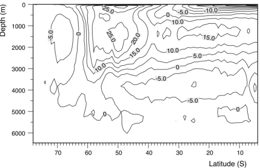
If changes in the wind stress produce significant changes in the ACC transport after only a few days, it is natural to ask how rapidly the Deacon Cell responds and what happens to the zonal momentum balance on the same timescale. As background, in Fig. 3 we plot the meridional overturning streamfunction for the control run, two days

5

into the analysis period.

The result is similar to that found in earlier studies (e.g. D ¨o ¨os and Webb, 1994). Near the surface at 50◦S there is a strong northward transport in the surface Ekman layer. Part of this is connected with the Deacon Cell. It appears to sink near 40◦S to a depth of 1500 m, returns south at depth and rises to the surface near the latitudes

10

of Drake Passage. The remainder is associated with the thermohaline circulation. It sinks near 40◦S and continues traveling north in the main thermocline. Later it returns southwards as North Atlantic Deep Water, appears to join the Deacon Cell circulation and also upwells near the latitudes of Drake Passage.

Unfortunately the overturning streamfunction cannot by itself be used to infer the path

15

of individual water particles. This is because the zonal averaging process loses impor-tant information. In the case of the thermohaline circulation the particles do roughly behave in the manner shown, but in the case of the Deacon Cell this is not true. D ¨o ¨os and Webb showed that in the FRAM model the Deacon Cell consisted of a series of small cells in which water particles travel northwards at one depth and then southwards

20

at a slightly deeper depth. At the top and bottom of the water column these effects do not cancel so the figure shows the northward and southward flows of the lightest and densest water masses. At intermediate levels the northward and southward flows can-cel and so the figure shows no net flow.

The overturning streamfunction is useful in showing where the ocean is gaining or

25

losing zonal momentum – or more accurately angular momentum around the Earth’s axis. At the surface the zonal wind stress increases the angular momentum of the water particles, which then move northwards to a latitude where their increased angular

(11)

OSD

3, 471–501, 2006

Printer-friendly Version Interactive Discussion momentum matches that of nearby particles in solid body rotation.

Where the stream lines indicate sinking, water particles actually are sinking carrying their angular momentum deeper into the water column. Exchanges of angular momen-tum between water particles of different density at the same depth are not shown, but where angular momentum is gained from or lost to the solid earth, through horizontal

5

pressure forces, this shows up as north-south flows at depth within the ocean. Thus the intermediate waters gain angular momentum as they move northwards in the ther-mocline and the southwards flowing water masses lose angular momentum as they cross the latitudes of Drake Passage below the level of the topography.

5.1 Changes in the Deacon Cell

10

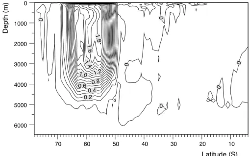
In Run 2, when the perturbation wind stress is added, the new overturning streamfunc-tion (not plotted) changes slightly but contains little new informastreamfunc-tion. More insight is obtained from the differences between the two streamfunctions. The difference at day two of the analysis period is plotted in Fig. 4. It shows a tight recirculation confined to the latitudes of increased wind stress.

15

In the surface layers the flow is northward, the extra transport at 60◦S being approx-imately 1.65 Sv. The extra Ekman transport in the surface layers due to the wind is given by,

T = Lτ/f,

where T is the transport, τ the wind stress, L the length of the line of latitude and f the Coriolis parameter.

L= 2πR cos θ, f = 2Ω sin θ, Ω = 2π/86164,

(12)

OSD

3, 471–501, 2006

EGU

where R is the radius of the earth, θ the latitude andΩ the angular velocity of the earth. If the wind stress τ is 0.1 dyne cm−2, then at a latitude of 60◦S, the expected increase in the Ekman transport is 1.58 Sv. Thus the observed transport is almost exactly that expected from theory.

At the northern limit of the main overturning cell, the streamfunction shows a

down-5

ward flux of water particles (and angular momentum) to depths below 3000 m. The flow then turns south, below the level of topography, and there is a final return flow to the surface which completes the cell.

It appears natural to describe this change in the overturning streamfunction as a change in the Deacon Cell. It is associated with the same topography and latitude

10

bands, it transfers wind stress downwards from the surface to the topography and, as very short time scales are involved, it does not involve changes in the density of water particles.

However there is one important difference. In the long term mean Deacon Cell dis-cussed byD ¨o ¨os and Webb (1994), the vertical movement of each water particle was

15

confined by the limits of its own small cell. This involved excursions of a few hundred metres and was consistent with the denisity differences and energetics involved.

In the present case the change in the current field has occurred too quickly for the baroclinic velocity field to be affected. So, if nothing else changed, in time water would be advected from the surface to great depth and back again. During the first few days,

20

during which water displacements are small, this is not a problem but in the long term changes in the density field will have a significant impact.

6 The sea-surface height field

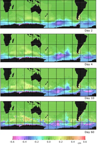
As discussed in the introduction, observations indicate that changes in ACC transport are associated with rapid changes in sea level all around Antarctica. In Fig. 5 we plot

25

the difference in the sea surface height field between the perturbation and control runs after two days, four days, ten days and sixty days.

(13)

OSD

3, 471–501, 2006

Printer-friendly Version Interactive Discussion The results show that initially there is a rapid drop in sea level all around

Antarc-tica. Low amplitude Kelvin and other waves propagate around the Pacific and Atlantic Oceans but the net change in sea level to the north is small.

After two days, an area of low sea level is found throughout a relatively narrow band around Antarctica. At most longitudes the northern limit of the band is well to the south

5

of the main ACC. The main changes to the current (not shown) are found in the region where the gradient of sea surface height difference is largest. Thus although a change in the wind produces a change in the total ACC transport, the extra current remains close to the Antarctic continent and is to a large extent independent of the main ACC.

Following day two and the initial fast response, the sea surface height field continues

10

to develop mainly through the formation of small scale structures. Thus the boundary between the low sea levels around Antarctica and the higher values off-shore becomes sharper. (An example is seen at day four and day ten just to the west of Drake Pas-sage). Elsewhere a graininess involving just a few grid points develops. (For example in the central South Pacific).

15

While this is happening some of the large scale features also become better defined. One of these features is the south Indian Ocean region of increased sea level. A sec-ond is the South-east Pacific region of low sea level which starts to extend northwards towards 30◦S but by day 60 is retreating back southwards. It may be significant that both features have similarities with the zero frequency ocean modes reported

previ-20

ously byWebb and de Cuevas(2002,2003).

Lines of increased sea level gradient also develop near the northern and southern limits of the band of increased wind stress. These are most noticable at day sixty, but can also be tracked back to day ten and day four. As discussed later they may be connected to the problem of matching the distribution of Ekman suction and Ekman

25

pumping with the contours of f /h.

It is also noticeable that the contours of sea surface height are affected by the ocean topography but that they do not follow lines of f /h. Instead the contours encircling Antarctica tend to follow the shallow mid-ocean ridge northwards in the South-west

(14)

OSD

3, 471–501, 2006

EGU

Pacific and later reattach to Antarctica via the deep oceanic basin to the east. A similar process appears to be occurring further east, with a northwards excursion in the shal-low topography, near Drake Passage, and a return southward fshal-low in the deeper South Atlantic.

7 The meridional velocity field

5

The results discussed so far show that the ACC transport, the meridional overturning streamfunction and the sea surface height field all respond very quickly to changes in the wind stress. The fast response implies that barotropic processes are involved, as the baroclinic processes associated with changes in the density field take far longer than two days to develop.

10

However it is not clear how the barotropic modes of the ocean, in which currents are depth independent, can generate the vertical flows seen in the overturning streamfunc-tion. To investigate how this happens, the differences in the north-south velocity field between the perturbation run and the control are plotted in Fig. 6 for days two and ten. Near the surface the figure shows a shallow northward flowing Ekman layer. Below

15

this the differences are primarily barotropic although there are some small baroclinic effects. The latter, seen as small regions of anomolous velocity, are found primarily in the top 1000 m. Their amplitudes increase slowly with time.

At day two, the barotropic flow is highly organised, with northward flow over regions of shallow topography and southward flow in the deep ocean basins. At day thirty

20

the flow is more complex but, as has been confirmed with a scatter plot, most of the northward flow occurs in shallow regions and most southward flow in the deep basins. As we discuss in the next section, at levels below the surface Ekman layer and above topography, the net north-south transport is almost zero. This is because the relatively strong and narrow northward flows over topography balance the weaker but

25

broad southward flows at the same depths in the deep ocean basins. Below the level of topography, there is a net southward flow and the Coriolis force associated with this

(15)

OSD

3, 471–501, 2006

Printer-friendly Version Interactive Discussion can set up a pressure field to act on the deep topography.

8 A barotropic Deacon Cell

If, below the Ekman layer, the change in the Deacon Cell is due just to the change in the barotropic velocity field then it should be possible to reproduce the overturn-ing streamfunction of Fig. 4 from the barotropic velocities. By barotropic velocity we

5

mean here the vertical average of the velocity field minus the wind driven Ekman layer contribution.

To check that this is true, we calculated the barotropic velocity at each point from the equation, v₀(θ, φ)= 1 h(θ, φ) Z0 −h(θ,φ) d z v (θ, φ, z) − τ_e(θ, φ)/f (θ), (1)

where v is the northwards component of velocity at longitude θ, latitude φ and depth z, h is the ocean depth, τ_eis the eastwards component of wind stress and f the Coriolis parameter. The overturning streamfunctionΨ is then given by,

Ψ =Z2π 0 d φ R sin θ Zz −h(θ,φ) d z0v₀(θ, φ), (2)

where R is the Earth’s radius.

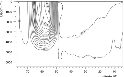
The predicted change in the overturning streamfunction at day two calculated from this equation is plotted in Fig. 7. The qualitative agreement with Fig. 4 is good but to obtain a quantitative measure of agreement we calculated E , the percentage variance unexplained. This is given by the equation,

E =100 Z Z

d z d φ (Ψ₀(θ, z) −Ψ(θ, z))2/ Z Z

(16)

OSD

3, 471–501, 2006

EGU

whereΨ₀is the original streamfunction difference.

At day two E has a value of 6.3%. When the calculation is repeated at day 10 the value is 2.5% and at day 30 it is reduced further to 0.6%. Similar results are obtained when, instead of using Eq. (1), the barotropic velocity is calculated either by integrating the velocity field below the top 20 m of the model (i.e. outside the surface Ekman layer)

5

or, assuming geostrophic balance, from the gradient of the sea surface height field. The results confirm that the change in the Deacon Cell is primarily a barotropic response of the ocean.

9 Time evolution of the momentum balance terms

In the above discussion it was implied that the extra pressure force on the deep

topog-10

raphy was equal to the extra zonal wind stress applied at the ocean surface and that this occurred on the same fast time scale that was associated with changes in the ACC transport, the Deacon Cell and changes in the sea surface height field. To check that this was true we calculated the different terms that contributed to the zonal momnetum equation along a line of latitude at 60.5◦S. Calculations were made using data in the

15

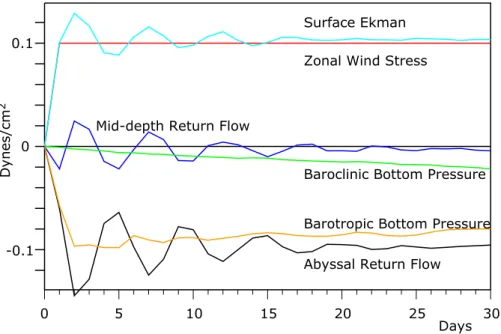
full archive datasets which were available at one day intervals. The results are plotted in Fig. 8.

The different terms calculated are: i) The total zonal wind stress W ,

W = Z

d φ R sin θ τ_x(θ, φ). (4)

ii) The integral of the Coriolis term in the three layers, where h₁ is the bottom of the model Ekman layer and h₂is the depth of the shallowest topographic feature. (In Fig. 8 these are 115 m and 1083 m respecively).

C₁= − Z2π 0 d φ R sin θ Zh1 0 d z v (θ, φ, z). (5)

(17)

OSD

3, 471–501, 2006

Printer-friendly Version Interactive Discussion C₂= − Z2π 0 d φ R sin θ Zh2 h1 d z v (θ, φ, z). (6) C₃= − Z2π 0 d φ R sin θ Zh h2 d z v (θ, φ, z). (7)

iii) The barotropic (sea surface height) contribution to the bottom pressure term,

P_ssh= Z2π 0 d φ gζ dh/d φ= − Z2π 0 d φ gh d ζ /d φ. (8)

iv) The baroclinic (internal density field) contribution to the bottom pressure term,

P_ρ= Z2π 0 d φ dh/d φ Z0 −h d z g ρ(θ, φ, z), (9)

where ρ is the density. The residual term due to viscosity is also plotted. Note that, for clarity, the signs have been chosen so that when they are in balance the surface wind stress term and the surface Ekman layer (or Coriolis) term have the same sign and

5

amplitude. Similarly when in balance the bottom Coriolis term and the bottom pressure terms also have the same sign and amplitude.

The figure shows three primary features. During the initial period, the Coriolis term increases to balance the surface wind stress. The surface flow is then affected by a slow oscillatory wave with a period of around five days which decays away after

10

approximately 25 days. The wave need to be investigated further but it is likely to be a barotropic Rossby wave excited by the change in surface forcing. The middle and bottom Coriolis terms show a similar behaviour, the oscillations in the middle layer dying away to nothing and those in the bottom layer leaving a residual which balances the near surface Ekman layer term.

(18)

OSD

3, 471–501, 2006

EGU

The bottom pressure terms also show a further longer period change. The SSH contribution initially increases to a level where it balances the surface wind stress. It then oscillates slightly after which it is seen to slowly reduce in amplitude. The second bottom pressure term due to the density field appears to compensate for this. Initially it has no significant effect but over the 30 day period of the runs it increases slowly so

5

by the end of the period it is 20% of the size of the surface wind stress term and is continuing to increase.

10 Discussion and conclusions

The present work has shown that when the zonal wind stress changes at the latitudes of Drake Passage, the ACC transport and sea levels around Antarctica all adjust to the

10

new forcing within a couple of days. Given the short time scale involved the process are expected to involve fast barotropic waves and this is confirmed by further investigations of the velocity field and the meridional overturning circulation. Thus in the case of the velocity field, outside the shallow wind-forced Ekman layer, all changes are to a good approximation independent of depth - they are primarily barotropic.

15

The long term changes in sea level observed with the present model are very sim-ilar to the Southern Ocean Mode, discovered and discussed byHughes et al.(1999). RecentlyWeijer and Gille (2005) analysed the frequency response of an unstratified Southern Ocean and showed that the mode was important at periods of more than a few days. They also found that it was not a free mode, i.e. it did not follow contours of

20

f /h. Thus all three models are exciting similar features but, on the basis of the present results, it is not obvious whether the models are seeing a single mode or a group of related modes.

The present results show that changes in the meridional overturning circulation are confined to the Deacon Cell and that they occur on the same fast time scale as the

25

change in the ACC transport. Thus any increase in the input of angular momentum from the atmosphere must be balanced, within a couple of days, by a compensating

(19)

OSD

3, 471–501, 2006

Printer-friendly Version Interactive Discussion increase in the loss of angular momentum to the solid Earth. The results give

fur-ther support to the idea that the primary role of the Deacon Cell is to transfer angular momentum vertically at the latitudes of Drake Passage.

The analysis also shows that, when the zonal wind stress increases, the ocean achieves the new balance barotropically by increasing the northward currents over

5

shallow topography and the southward currents in the deep basins. At depths between the Ekman layer and the shallowest topography, the total transport per unit depth bal-ances out to zero, but there remains an extra southward flow in the deeper layers which balances the increased northward flow in the surface Ekman layer. It is the horizontal pressure gradients associated with this deep flow which transfer the increased flux of

10

angular momentum to the topography and the solid Earth.

Further work is required to fully understand how the new balance is achieved. Initially the wind driven Ekman transport reduces sea level in the south and increases it in the north. Once a steady state is achieved, this results in regions of Ekman suction and Ekman pumping uniformly distributed along lines of latitude at the northern and

15

southern limits of the band of modified wind forcing.

However if the resulting barotropic flow is matched to the distribution of Ekman pump-ing in the north and then carries the excess flow to the south, it is difficult to see, given the complex topography of the Souther Ocean, how if the flow follows lines of constant f /h, it also exactly matches the band of Ekman suction in the south. A full solution

20

may involve other processes. One possibility is the presence of barotropic gyres, with the equivalent of western boundary currents in which the flow crosses contours of f /h. These would involve barotropic Rossby waves and so may take time to develop. It is thus interesting to note that the sea surface height field shows structures developing at the latitudes of Ekman pumping and suction, so it is concievable that these are a result

25

of such a process.

There is also the question of how and why changes in the wind (or changes in the Ek-man transport), affect the strength of the ACC. The fact that the response is barotropic should make it easier to understand the fast response results presented here. One

(20)

ap-OSD

3, 471–501, 2006

EGU

proach is discussed in Appendix A, where estimates of the mean depths of the shallow and deep regions of ocean are used to estimate the size of the north-south barotropic transports in each of these regions. An assumption about the way the regions are connected then gives a very approximate estimate of the change in the strength of the ACC. Despite the crude approximations the resulting estimate is not unreasonable.

5

The results also indicate the possibility that not all of the Ekman transport return flow need generate changes in the ACC transport. The sea surface height (and barotropic velocity) plots show recirculation regions in the South Indian Ocean and elsewhere and it is possible that wind stress events in these regions may only produces changes in the circulation within the region.

10

Finally a major conclusion of the present work is that a change in the barotropic flow field is sufficient to balance a change in the zonal wind stress at the latitudes of Drake Passage. As far as we know this is a new result, previous studies of the momentum balance all assuming that only baroclinic processes were involved, in the form of mesoscale eddies, large scale meanders of the ACC or changes in the large

15

scale thermohaline circulation. The work byHughes et al.(1999,2003) on sea level around Antarctica and its correlation with the ACC transport did essentially question this assumption and this new work has confirmed their suspicions.

That is not to say that the baroclinic theories are wrong. In the ocean, the time scale of baroclinic processes ranges from a few weeks, for changes to mesoscale eddies,

20

to hundreds of years for changes to the large scale thermohaline circulation. In the present case we expect baroclinic processes to be involved in two ways. First changes in the horizontal barotropic flow field will change the distribution of density in the ocean and this will inevitably generate baroclinic waves. The difference flow field shown in Fig. 6, shows anomalies within the ocean which may be a result of such waves.

25

Secondly the requirements of continuity mean that there is a change in the vertical velocity fields at the northern and southern limits of the band of increased winds. Over a period of a few days the vertical displacements are small but in time the changed buoyancy forces will resist the overturning (Deacon Cell) circulation and start

(21)

generat-OSD

3, 471–501, 2006

Printer-friendly Version Interactive Discussion ing their own baroclinic circulation. Again the details of how this happens needs to be

investigated further but we expect it to result in the shallow overturning cells discussed byD ¨o ¨os and Webb(1994).

Both processes will have the effect of changing the bottom pressure distribution and so allow the baroclinic field to contribute to the downward transfer of momentum (or

5

strictly speaking angular momentum). In the present study we found that at then end of thirty days the baroclinic contribution to the momentum transfer had reached 20% of the total.Hughes et al.(2003) estimated that after a year, baroclinic processes became dominant. The present results are consistent with such a timescale.

Appendix A An estimate of the change in the ACC transport

10

Let us approximate the model results by assuming that outside the Ekman layer, the change in the current field consists of a single barotropic current with two large mean-ders, one in the South Pacific and the second in the South Atlantic. In each of these meanders the current is assumed to flow northwards in a region with an average depth of 2400 m and returns southwards at an average depth of 4800 m (see Fig. 6). Assume that the Coriolis parameter f is constant and that there is a fixed sea level drop δh across the current. The total transport per unit depth T is given by,

T = g δh/f, (A1)

where g is gravity. Thus T is a constant.

Let E be the change in the northward Ekman transport, H₁ be the the mean depth in the shallow regions with northward transport and H₂ the mean depth in the deep regions of southward transport. Let the corresponding full depth barotropic transports be T₁and T₂. Then,

(22)

OSD

3, 471–501, 2006

Printer-friendly Version Interactive Discussion EGU and T₁/H₁= T₂/H₂. (A3) Thus, T₁= 0.5 E H₁/(H₂− H₁), T₂= 0.5 E H₂/(H₂− H₁). (A4)

For the depth values given above, this becomes, T₁= E/2,

T₂= E. (A5)

In Drake Passage the additional barotropic current is attached to the continental shelf prior to turning northwards following shallow topography. Therefor the extra flux through Drake Passage should correspond to T₁. The simple theory thus predicts that the short term increase in ACC transport due to changes in the wind should be roughly half the increase in Ekman transport.

5

The model showed that an increase in the zonal wind of 0.1 dyne cm−2 produces an increase in the Ekman transport of 1.58 Sv at 60◦S and an increase in the ACC transport of 0.87 Sv. The good agreement with the above theory may be fortuitous, the full circulation with its recirculation regions being much more complex than that of the simple model, but it does give an indication as to why the increase in the ACC transport

10

is so much less than the increase in Ekman transport.

References

Bryan, K.: A numerical method for the study of the circulation of the world ocean, Journal of Computational Physics, 4, 347–376, 1969. 475

(23)

OSD

3, 471–501, 2006

Coward, A. C. and de Cuevas, B. A.: The OCCAM 66 Level Model: Physics, Initial Conditions and External Forcing, Southampton Oceanography Centre, Internal Report No 99, 58pp, 2005. 475

Cox, M. D.: A primitive equation 3-dimensional model of the ocean, Tech.Rep. 1, Geophys. Fluid Dyn. Lab, Natl. Oceanic and Atmos. Admin., Princeton Uni. Press, Princeton, N.J.,

5

1984. 475

D ¨o ¨os, K. and Webb, D. J.: The Deacon Cell and other Meridional Cells of the Southern Ocean, Journal of Physical Oceanography, 24, 429–442, 1994. 473,479,481,490

FRAM Group: An eddy-resolving model of the Southern Ocean, EOS Transactions of the Amer-ican Geophysical Union, 72, 169–175, 1991. 473

10

Gille, S. T.: Dynamics of the Antarctic Circumpolar Current: Evidence for topographic effects from Altimeter data and numerical model output, PhD thesis, Massachusetts Institute of Technology and Woods Hole Oceanographic Institution, 217pp, 1995. 473

Gouretski, V. V. and Jancke, K.: A new hydrographic data set for the South Pacific: synthesis of WOCE and historical data, WHP SAC Technical Report No.2, WOCE Report No. 143/96,

15

unpublished manuscript, 1996. 476

Griffies, S. M., Gnanadesikan, A., Dixon, K. W., Dunne, J. P., Gerdes, R., Harrison, M. J., Rosati, A., Russell, J. L., Samuels, B. L., Spelman, M. J., Winton, M., and Zhang, R.: For-mulation of an ocean model for global climate siFor-mulations, Ocean Science, 1, 45–79, 2005.

475 20

Hughes, C. W., Meredith, M. P., and Heywood, K. J.: Wind-Driven Transport Fluctuations through Drake Passage: A Southerrn Mode, Journal of Physical Oceanography, 29, 1971– 1992, 1999. 474,475,487,489

Hughes, C. W., Woodworth, P. L., Meredith, M. P., Pyne, A. R., Stepanov, V., and Whitworth, T.: Coherence of Antarctic sea levels, Southern Hemisphere Annular Mode, and flow through

25

Drake Passage, Geophys. Res. Lett., 30(9), 1464, doi:10.1029/2003GL017240, 2003. 474,

489,490

Ivchenko, V. O., Richards, K. J., and Stevens, D. P.: The Dynamics of the Antarctic Circumpolar Current, Journal of Physical Oceanography, 26, 753–774, 1996. 473

Johnson, G. C. and Bryden, H. L.: On the size of the Antarctic Circumpolar Current, Deep-Sea

30

Res., 36, 39–53, 1989. 473

Marshall, J., Olbers, D., Ross, H., and Wolf-Gladrow, D.: Potential Vorticity Constraints on the dynamics and hydrography of the Southern Ocean, Journal of Physical Oceanography, 23,

(24)

OSD

3, 471–501, 2006

EGU 465–487, 1993. 473

Munk, W. H. and Palm ´en, E.: Note on dynamics of the Antarctic Circumpolar Current, Tellus, 3, 53–55, 1951. 472,474

Rintoul, S. R., Hughes, C. W., and Olbers, D.: The Antarctic Circumpolar Current System, p. 271–302, in: Ocean Circulation and Climate, edited by: Siedler, G., Church, J., and Gould,

5

J., Academic Press, San Diego, 2001. 473

Semtner, A. J.: An oceanic general circulation model with bottom topography, Technical Report No. 9, Dept of Meteorology, UCLA, Los Angeles, CA 90095, 1974. 475

Siefridt, L. and Barnier, B.: Banque de Donnes AVIS Vent/flux: Climatologie des Analyses de Surface du CEPMMT, ORSTOM Report 91 1430 025, Toulouse, 1993. 476

10

Steele, M., Morley, R., and Ermold, W.: PHC: A global ocean hydrography with a high quality Arctic Ocean, J. Clim., 14, 2079–2087, 2001. 476

Stevens, D. P. and Ivchenko, V. O.: The zonal momentum balance in an eddy-resolving general-circulation model of the Southern Ocean, Quarterly Journal of the Royal Meteorological So-ciety, 123, 929–951, 1996. 473

15

Webb, D. J.: A simple model of the effect of the Kerguelen Plateau on the strength of the Antarctic Circumpolar Current, Geophysical and Astrophysical Fluid Dynamics, 70, 57–84, 1993. 473

Webb, D. J.: The vertical advection of momentum in Bryan-Cox-Semtner ocean general circu-lation models, Journal of Physical Oceanography, 25(12), 3186–3195, 1995. 475

20

Webb, D. J., de Cuevas, B., and Richmond, C.: Improved advection schemes for ocean models, J. Atmos. Ocean. Tech., 15, 1171–1187, 1998. 475

Webb, D. J. and de Cuevas, B. A.: An Ocean Resonance in the Indian Sector of the Southern Ocean, Geophys. Res. Lett., 29(14), 9-1–9-2, 2002. 482

Webb, D. J. and de Cuevas, B. A.: On the region of large SSH variability in the Southeast

25

Pacific, Journal of Physical Oceanograph, 33(5), 1044–1056, 2003. 482

Weijer, W. and Gille, S. T.: Ajustment of the Southern Ocean to Wind Forcing on Synoptic Time Scales, Journal of Physical Oceanography, 35, 2076–2089, 2005. 487

(25)

OSD

3, 471–501, 2006

Printer-friendly Version Interactive Discussion 0 1 2 3 4 5 6 7 8 9 10 Years 0 20 40 60 80 100 120 140 160 Tr an sp or t ( Sv )

Fig. 1. Drake Passage transports during the spin up and test periods. The lines are: Black –

the control run; Red – perturbation run, zonal wind stress increased by 0.1 dyne cm−2 at the latitudes of Drake Passage; Green – zonal wind stress set to zero at the same latitudes; Blue – wind stress set to zero everywhere. Transport in Sverdrups (1 Sv=106

(26)

OSD

3, 471–501, 2006

Printer-friendly Version Interactive Discussion EGU -10 0 10 20 30 40 50 60 70 120 130 140 150 Days Tr an sp or t ( Sv )

Fig. 2. Drake Passage transport during the analysis period. The lines are: Black – the control

run; Red – perturbation run, zonal wind stress increased by 0.1 dyne cm−2 at the latitudes of Drake Passage; Green – zonal wind stress set to zero at the same latitudes; Blue – wind stress set to zero everywhere. Days measured relative to day 3690 at the start of the analysis period. Transport in Sverdrups (1 Sv=106m3s−1).

(27)

OSD

3, 471–501, 2006

Printer-friendly Version Interactive Discussion 70 60 50 40 30 20 10 6000 5000 4000 3000 2000 1000 0 Latitude (S) D ep th (m ) -10.0 -5 .0 -5.0 -5.0 -5.0 5.0 0 0 0 0 0 10.0 10.0 10.0 15.0 15.0 20.0 25.0 25_.0

Fig. 3. Meridional overturning streamfunction for the control run at day 3692, after two days of

the analysis period. Contour values are in Sverdrups (1 Sv=106

(28)

OSD

3, 471–501, 2006

Printer-friendly Version Interactive Discussion EGU 0 0 0 0 0 0 0.20.4 0.6 0.8 1.0 1.4 1.6 1.8 1.2 70 60 50 40 30 20 10 6000 5000 4000 3000 2000 1000 0 Latitude (S) D ep th (m )

Fig. 4. Difference in the meridional overturning streamfunction between the perturbation run

(Run 2 – an additional 0.1 dyne cm−2 wind stress at the latitudes of Drake Passage) and the control run after two days.

(29)

OSD

3, 471–501, 2006

Printer-friendly Version Interactive Discussion -0.4 -0.6 -0.2 0.0 0.2 0.4 _{cm 0.6} Day 4 Day 2 Day 60 Day 10

Fig. 5. Difference in sea level between the perturbation run and the control run after two days,

(30)

OSD

3, 471–501, 2006

Printer-friendly Version Interactive Discussion EGU 0.0 0.1 0.2 cm/s Day 10 Day 2 -0.2 0 90 180 270 360 0 90 180 270 360 0 2000 4000 6000 0 2000 4000 6000 -0.1

Fig. 6. Zonal section through Drake Passage (60.5◦S) showing the difference in the north

components of velocity between the perturbation run and the control run after two days and after ten days. Depth in metres, longitude in degrees east.

(31)

OSD

3, 471–501, 2006

Printer-friendly Version Interactive Discussion 0 0 -0.1 0.5 0.1 1.0 1.5 1 .7 70 60 50 40 30 20 10 6000 5000 4000 3000 2000 1000 0 Latitude (S) D ep th (m )

Fig. 7. The predicted change in the overturning streamfunction between the perturbation run

and the control run at day 2 of the analysis period calculated from the barotropic velocity and the surface wind stress.

(32)

OSD

3, 471–501, 2006

Printer-friendly Version Interactive Discussion EGU 0 5 10 15 20 25 30 0 0.1 -0.1 Days D yn es /c m 2 Surface Ekman Zonal Wind Stress

Mid-depth Return Flow

Baroclinic Bottom Pressure Barotropic Bottom Pressure Abyssal Return Flow

Fig. 8. Mean value per unit area of terms contributing to the zonally integrated momentum

balance at the latitude of Drake Passage. See section 9 for definitions. Values are calculated and plotted at intervals of one day. Additional terms not shown (i.e. horizontal viscosity and bottom friction) have negligable amplitude at the scale plotted.