HAL Id: hal-00302687
https://hal.archives-ouvertes.fr/hal-00302687
Submitted on 20 Dec 2005
HAL is a multi-disciplinary open access
archive for the deposit and dissemination of
sci-entific research documents, whether they are
pub-lished or not. The documents may come from
teaching and research institutions in France or
abroad, or from public or private research centers.
L’archive ouverte pluridisciplinaire HAL, est
destinée au dépôt et à la diffusion de documents
scientifiques de niveau recherche, publiés ou non,
émanant des établissements d’enseignement et de
recherche français ou étrangers, des laboratoires
publics ou privés.
Experiments on transitions of baroclinic waves in a
differentially heated rotating annulus
Th. von Larcher, C. Egbers
To cite this version:
Th. von Larcher, C. Egbers. Experiments on transitions of baroclinic waves in a differentially heated
rotating annulus. Nonlinear Processes in Geophysics, European Geosciences Union (EGU), 2005, 12
(6), pp.1033-1041. �hal-00302687�
SRef-ID: 1607-7946/npg/2005-12-1033 European Geosciences Union
© 2005 Author(s). This work is licensed under a Creative Commons License.
Nonlinear Processes
in Geophysics
Experiments on transitions of baroclinic waves in a differentially
heated rotating annulus
Th. von Larcher and C. Egbers
Department of Aerodynamics and Fluid Mechanics, Brandenburg University of Technology Cottbus, 03046 Cottbus, Germany Received: 4 October 2005 – Revised: 28 November 2005 – Accepted: 28 November 2005 – Published: 20 December 2005 Part of Special Issue “Turbulent transport in geosciences”
Abstract. Experiments of baroclinic waves in a rotating, baroclinic annulus of fluid are presented for two gap widths. The apparatus is a differentially heated cylindrical gap, ro-tated around its vertical axis of symmetry, cooled from within, with a free surface, and filled with de-ionised water as working fluid. The surface flow was observed with visu-alisation technique while thermographic measurements gave a detailed understanding of the temperature distribution and its time-dependent behaviour.
We focus in particular on transitions between different flow regimes. Using a wide gap, the first transition from axisymmetric flow to the regular wave regime was charac-terised by complex flows. The transition to irregular flows was smooth, where a coexistence of the large-scale jet-stream and small-scale vortices was observed. Furthermore, temper-ature measurements showed a repetitive separation of cold vortices from the inner wall. Experiments using a narrow gap showed no complex flows but strong hysteresis in the steady wave regime, with up to five different azimuthal wave modes as potential steady and stable solutions.
1 Introduction
Baroclinic waves are known to be of particular importance for the transport of heat and momentum in the earth’s atmo-sphere and in oceans and also atmospheric flows on other ter-restrial planets may affected by baroclinic instability. A suit-able laboratory model for the mid-latitude large-scale flow phenomena in the earth’s atmosphere is the differentially heated rotating annulus of fluid as mentioned for example in an article by Fultz (1961). Since the pioneering investiga-tions by Hide (1958) of the baroclinic annulus experiment, baroclinic waves have been investigated in the annulus not only in numerous experimental studies but also theoretically, e.g. Lorenz (1962), and numerically, for example by Miller
Correspondence to: Th. von Larcher
and Gall (1983). Methods of nonlinear time series analy-sis were used to investigate the dynamics of baroclinic wave flows for example by Read et al. (1992) and Fr¨uh and Read (1997), who used time series of temperature data of the fluid interior, as Sitte and Egbers (2000) used velocity time se-ries data which were acquired by the optical Laser Doppler Velocimetry technique. Recent theoretical work by Lewis and Nagata (2004) focussed on the linear stability analysis while ongoing numerical work by Randriamampianina, et al. (2005)1considered air as a working fluid in contrast to a liq-uid in the annulus.
Since the flow regime that develops in the cylindrical gap depends on the forcing parameters, i.e. on the radial temper-ature gradient between its vertical endwalls, 1T , and on the rotation rate of the apparatus, , a usual form of displaying the characteristics of the fluid flow as a function of these two parameters is the two-parameter regime diagram spanned by the dimensionless Taylor number T a as abscissa, T a ∝ 2, and thermal Rossby number Ro as ordinate, Ro ∝ 1T
2.
Vis-cosity as one of the physical properties of the fluid is the third key parameter and has significant effects on the regime dia-gram and on transitions between different flow regimes as experimental studys of e.g. Fowlis and Hide (1965) and Fein and Pfeffer (1976) have shown.
The regime diagram for fluids like water (Fig. 1) typically displays the well investigated anvil shape which characterises the transition from axisymmetric flow to regular baroclinic waves (e.g. Hide and Mason, 1975). While the flow in the lower symmetric regime is stabilised by diffusive effects, ax-isymmetric flow in the upper symmetric regime is stable due to stratification. Geostrophic turbulence, characterised by spatially irregular, aperiodic flows, is found at high rotation rates. Flows in the regular wave regime are found to be ei-ther steady or time-dependent as the latter undergo changes in amplitude or shape for example, denoted as ‘amplitude 1Randriamampianina, A., Fr¨uh, W.-G., Maubert, P., and Read,
P. L.: DNS of bifurcations to low-dimensional chaos in an air-filled rotating baroclinic annulus, J. Fluid Mech., submitted, 2005.
1034 Th. von Larcher and C. Egbers: Experiments on transitions of baroclinic waves 10 10 10 10 1 10 0.01 0.001 th. Rossby number Ro 0.1 5 6 7 8 Taylor number Ta
Fig. 1. Parameter space for water (Fowlis and Hide, 1965,
modi-fied).
vacillation’ (AV ) and ‘structural vacillation’ (SV ), respec-tively, as well as more types of complex flow patterns are known to exist in the baroclinic annulus like ‘modulated am-plitude vacillations’ (MAV ) and various multi-mode states (e.g. Hide and Mason, 1975; Pfeffer et al., 1980; Hignett et al., 1985; Read et al., 1992; Fr¨uh and Read, 1997). Partic-ularly, Fr¨uh and Read (1997), who studied nonlinear aspects of complex flows within the regular wave regime, reported on other types of flow states where an intermittent bursting of the flow field were observed and of those in which the flow alternated between two zonal wave modes. Even though SV -like flows appear to be regular with some weak spatially lo-calized instabilities it seems that they can not be described by low-dimensional dynamics as an estimate of the dimension failed, contrary to AV and MAV flows which were found to be quasi-periodic and usually chaotic resp. (Guckenheimer, 1983; Read et al., 1992; Fr¨uh and Read, 1997).
Hysteresis, which describes the dependence of flow regimes on initial conditions so that more than one wave number or flow state can occur at identical forcing param-eters, is a well known phenomenon in such annulus experi-ments and is generally observed between different azimuthal wave modes using a free surface (e.g. Sitte and Egbers, 2000; von Larcher and Egbers, 2005) and in the rigid lid case (e.g. Cole, 1971; Hignett et al., 1985). Also, the transition from the upper symmetric regime to the ‘steady’ wave regime was observed to be affected by hysteresis (Fultz et al., 1959, as reported in Miller and Butler, 1991), but investigations of the transition from the lower symmetric regime to the regular wave regime with a rigid lid generally found no hysteresis (W.-G. Fr¨uh, private communication).
This study is concerned with the effect of the gap width on transition between wave numbers, in particular the degree of hysteresis involved and complex vacillations. The results are based on conventional flow visualisation but also on ther-mographic measurements which show the temperature field at the surface of the fluid. The apparatus and measurement techniques are described in the following section, while the results for the wide gap and the narrow gap experiments are
heating coil
temperature control
supervision thermostat
rotation rate control
co−rotating
camera
pump
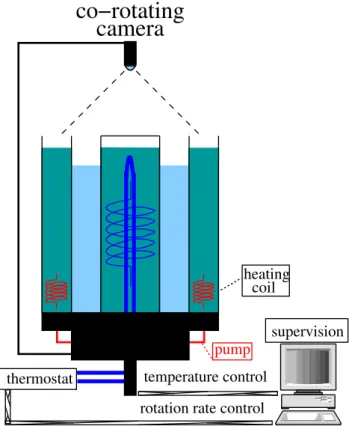
Fig. 2. Sketch of the experiment set-up.
presented in Sects. 3.1 and 3.2, respectively. The paper is then concluded with a discussion section and a conclusion.
2 Experimental setup
The set-up (Fig. 2) consisted of a tank with three concentric cylinders which was built on a turntable and rotated around its vertical axis of symmetry. The inner cylinder was made of anodised aluminium, the middle and outer one were made of borosilicate glass. The cylindrical gap (the middle chamber) had a flat bottom topography while its surface was free. A temperature difference between the vertical end walls of the gap was realised by heating the fluid in the outer chamber by a heating coil and cooling the fluid in the inner chamber using a thermostat. De-ionised water is used as working fluid.
The temperature of the inner and outer cylinder and also the rotation rate of the apparatus was controlled by the ex-periment software which was programmed in LabVIEW®, as was the co-rotating camera, which allowed for automated long-time measurements with smooth parameter variations. Two temperature sensors (resolution 0.07 K) were integrated in the upper and lower part of the inner gap wall and four sen-sors of the same model were mounted in the outer cylinder close to the outer gap wall in mid-height and with distance of
π
2 in azimuth.
Geometric parameters of the experimental setup, typical experiment conditions and physical properties of the fluid are shown in Table 1. Generally, the observable wave number
mis restricted by the dimensions of the gap, as Hide and Mason (1970) found an empirical law of the minimum and maximum wave number, mmin≤m≤mmax, that is in modi-fied form 1 4·π · (b + a) (b − a) ≤m ≤ 3 4 ·π · (b + a) (b − a), (1)
which results in (2) 1.7≤m≤5.2 (5) for the wide gap and (7) 6.8≤m≤20.3 (20) for the narrow gap (integral wave numbers in parenthesis).
A co-rotating U SB camera was used to observe the sur-face flow from above which was then visualised with alu-minium particles. For thermographic measurements of the surface temperature distribution, this camera was removed and a non-rotating heat sensitive camera of high quality was mounted above the tank (resolution ±0.03 K, absolute accu-racy <±2 K, 240 rows per picture, 360 pixel per row, 16 bit A/D converter).
Experiments with a wide gap were done applying visuali-sations of the surface flow as well as thermographic measure-ments. Using the narrow gap, the thermographic camera was not available and only visualisation technique was applied. Pictures of the surface flow were taken every 30 s as records up to 60 s were taken usually every 1200 s. The sample in-terval of thermographic measurements was 30 s.
The Taylor number and thermal Rossby number describe the two principal variables, i.e. the horizontal density gra-dient 1ρ due to the imposed temperature gragra-dient and the rotation rate, respectively, by
T a = 4
2(b − a)5
ν2d and Ro =
g d 1ρ ρ 2(b − a)2, with a and b as inner and outer radius of the gap, d as fluid depth, ρ as average density, g as acceleration due to grav-ity, ν as kinematic viscosity. The Prandtl number, defined by P r=νκ, κ as thermal conductivity, describes the physical properties of the fluid (P r=7 for the working fluid). Both experiments used a fluid depth of d=135 mm resulting in a radius ratio, η=ab, and aspect ratio, 0=(b−a)d of η=0.38 and 0=1.8 for the wide gap experiments, and η=0.79 and 0=5.4 for the small gap experiments.
By keeping the temperature gradient fixed and varying the rotation rate of the apparatus, regime sequences can be de-fined which represent cuts of the parameter space. The spin-up time was found to be less than 30 min for steady waves and up to 40 min for complex flows. Observations were done up to three hours per parameter point, extended partly to four hours in complex flow regimes. Due to limited availabil-ity time of the thermographic camera, temperature measure-ments were restricted to two hours per parameter point.
To define a reference temperature gradient, we used the averaged temperature difference measured in the axisymmet-ric flow regime close to the transition to the first instability, i.e. 1T =7.5 K in the wide gap case and 1T =6.7 K in the narrow gap case. In practice, the thermal Rossby number was individually calculated for each parameter point using the averaged temperature gradient which was calculated from
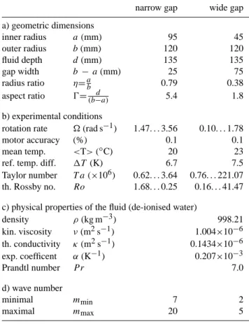
Table 1. a) Geometric parameters of the experimental setup, b)
typical experiment conditions, c) physical properties of the working fluid at T = 20◦C, p = 105Pa, d) integral wave numbers as derived from Eq. (1).
narrow gap wide gap a) geometric dimensions inner radius a (mm) 95 45 outer radius b(mm) 120 120 fluid depth d(mm) 135 135 gap width b − a(mm) 25 75 radius ratio η=ab 0.79 0.38 aspect ratio 0=(b−a)d 5.4 1.8 b) experimental conditions
rotation rate (rad s−1) 1.47. . . 3.56 0.10. . . 1.78 motor accuracy (%) 0.1 0.1 mean temp. <T> (◦C) 20 23 ref. temp. diff. 1T (K) 6.7 7.5 Taylor number T a (×106) 0.62. . . 3.64 0.76. . . 221.07 th. Rossby no. Ro 1.68. . . 0.25 0.16. . . 41.47 c) physical properties of the fluid (de-ionised water)
density ρ(kg m−3) 998.21 kin. viscosity ν(m2s−1) 1.004×10⁻⁶ th. conductivity κ(m2s−1) 0.1434×10⁻⁶ exp. coefficent α(K−1) 0.207×10⁻³ Prandtl number P r 7.0 d) wave number minimal mmin 7 2 maximal mmax 20 5
the permanent temperature measurements. Deviations of the temperature gradient was found to be within ±0.1 K in nar-row gap experiments and ±0.2 K in wide gap experiments, 2.1 Narrow gap temperature control
Using the narrow gap, the imposed temperature gradient could not be kept constant due to technical reasons and was found to be affected by the flow state in a significant manner for lower and medium rotation rates.
Figure 3 shows logs of the temperature gradient for in-creasing and dein-creasing Taylor numbers. The temperature drop and jump, respectively, at the transition from axisym-metric flow to the wavy flow regime was substantial. In case of increasing Taylor numbers, additional drops of the tem-perature gradient, weak but noticable in amplitude, were ob-served up to m=8. Here, it was possible to assign specific temperature differences to wave numbers from m=0 to m=8. While wave number m=5 was stable for 6.5 K≥1T ≥6.25 K, modes of m=6 and m=7 were restricted to 1T ≈6.17 K and 1T ≈6.07 K, respectively. For higher wave numbers, the temperature gradient remained constant at approx. 5.9 K.
In case of decreasing Taylor number, the temperature log look similar but the gradient appeared to increase not
1036 Th. von Larcher and C. Egbers: Experiments on transitions of baroclinic waves 0 500 1000 1500 2000 2500 3000 3500 4000 5.5 5.75 6 6.25 6.5 6.75 7 7.25 7.5
consecutive number (minutes)
temperature difference ( K ) 1.02×10⁶≤ Ta ≤ 1.97×10⁶ 1.89×10⁶≤ Ta ≤ 3.22×10⁶ 6.17×10⁵≤ Ta ≤ 1.26×10⁶ m=7 m=6 m=0 → m=5 m=8 and m=9 m=12 m = wave number m=9,10,11,12 first instability at Ta = 7.44 ×10⁵ m=0 → m=5 (visualisations) 0 500 1000 1500 2000 2500 3000 5.5 5.75 6 6.25 6.5 6.75 7 7.25 7.5
consecutive numbers (minutes)
temperature difference ( K ) 3.64×10⁶≥ Ta ≥ 3.03×10⁶ 3.12×10⁶≥ Ta ≥ 2.21×10⁶ 2.29×10⁶≥ Ta ≥ 1.39×10⁶ 1.39×10⁶≥ Ta ≥ 7.56×10⁵ 8.83×10⁵≥ Ta ≥ 6.17×10⁵ first instability at Ta = 7.44 ×10⁵ m=7 → m=0 (visualisations) m = wave number m=7 → m=0 m=13/12 m=13/12m=12 and m=11 m=12,11,10,9,7
Fig. 3. Narrow gap experiments. Log of the temperature gradient
for the increase (upper subfigure) and decrease (lower one) of the Taylor number. Parameter runs as well as wave numbers m are as-signed to temperature logs by colors.
stepwise but smoothly, especially for wavy flows of m=11 to m=7. Therefore, a correlation of wavy flow pattern and temperature gradient have not been undertaken. Generally, although the preset forcing parameters were the same, there was a systematic difference in the temperature gradient for increasing and decreasing Taylor numbers of round about 0.15 K.
3 Results
3.1 Wide gap experiments
The regime diagram as defined by visualisation is shown in Fig. 4 and photographs of particular flow patterns of m=0 to m=4 which was observed at different parameter points are shown in Fig. 5, where sketches of the flow states are drawn in for clarification. Generally, wavy flows up to m=4 were found but the overall steady flow regime was domi-nated by a m=3 mode. The critical Taylor number which marks the onset of the first instability was determined to be T ac=6.33×10⁶where the transition from axisymmetric flow
Tac= 6.33 × 10⁶ ↑ Tac 3 × 10⁶ 107 108 3 × 10⁸ Taylor number Ta
m=0
l2
2/3I
l l3
.. .. .. .. .. .. .. .. .. .. .. .. .. .. .. .. .. .. .. .. .. .. .. .. .. .. .. .. .. .. .. .. .. .. .. .. .. .. .. .. .. .. .. .. .. .. .. .. .. .. .. .. .. .. .. .. .. .. .. .. .. .. . .. .. .. .. .. .. .. .. .. .. .. .. .. .. .. .. .. .. .. .. .. .. .. .. .. .. .. .. .. .. .. .. .. .. .. .. .. .. .. .. .. .. .. .. .. .. .. .. .. .. .. .. .. .. .. .. .. .. .. .. .. .. . .. .. .. .. .. .. .. .. .. .. .. .. .. .. .. .. .. .. .. .. .. .. .. .. .. .. .. .. .. .. .. .. .. .. .. .. .. .. .. .. .. .. .. .. .. .. .. .. .. .. .. .. .. .. .. .. .. .. .. .. .. .. . .. .. .. .. .. .. .. .. .. .. .. .. .. .. .. .. .. .. .. .. .. .. .. .. .. .. .. .. .. .. .. .. .. .. .. .. .. .. .. .. .. .. .. .. .. .. .. .. .. .. .. .. .. .. .. .. .. .. .. .. .. .. . .. .. .. .. .. .. .. .. .. .. .. .. .. .. .. .. .. .. .. .. .. .. .. .. .. .. .. .. .. .. .. .. .. .. .. .. .. .. .. .. .. .. .. .. .. .. .. .. .. .. .. .. .. .. .. .. .. .. .. .. .. .. . .. .. .. .. .. .. .. .. .. .. .. .. .. .. .. .. .. .. .. .. .. .. .. .. .. .. .. .. .. .. .. .. .. .. .. .. .. .. .. .. .. .. .. .. .. .. .. .. .. .. .. .. .. .. .. .. .. .. .. .. .. .. . .. .. .. .. .. .. .. .. .. .. .. .. .. .. .. .. .. .. .. .. .. .. .. .. .. .. .. .. .. .. .. .. .. .. .. .. .. .. .. .. .. .. .. .. .. .. .. .. .. .. .. .. .. .. .. .. .. .. .. .. .. .. . .. .. .. .. .. .. .. .. .. .. .. .. .. .. .. .. .. .. .. .. .. .. .. .. .. .. .. .. .. .. .. .. .. .. .. .. .. .. .. .. .. .. .. .. .. .. .. .. .. .. .. .. .. .. .. .. .. .. .. .. .. .. . .. .. .. .. .. .. .. .. .. .. .. .. .. .. .. .. .. .. .. .. .. .. .. .. .. .. .. .. .. .. .. .. .. .. .. .. .. .. .. .. .. .. .. .. .. .. .. .. .. .. .. .. .. .. .. .. .. .. .. .. .. .. . .. .. .. .. .. .. .. .. .. .. .. .. .. .. .. .. .. .. .. .. .. .. .. .. .. .. .. .. .. .. .. .. .. .. .. .. .. .. .. .. .. .. .. .. .. .. .. .. .. .. .. .. .. .. .. .. .. .. .. .. .. .. . .. .. .. .. .. .. .. .. .. .. .. .. .. .. .. .. .. .. .. .. .. .. .. .. .. .. .. .. .. .. .. .. .. .. .. .. .. .. .. .. .. .. .. .. .. .. .. .. .. .. .. .. .. .. .. .. .. .. .. .. .. .. . .. .. .. .. .. .. .. .. .. .. .. .. .. .. .. .. .. .. .. .. .. .. .. .. .. .. .. .. .. .. .. .. .. .. .. .. .. .. .. .. .. .. .. .. .. .. .. .. .. .. .. .. .. .. .. .. .. .. .. .. .. .. . .. .. .. .. .. .. .. .. .. .. .. .. .. .. .. .. .. .. .. .. .. .. .. .. .. .. .. .. .. .. .. .. .. .. .. .. .. .. .. .. .. .. .. .. .. .. .. .. .. .. .. .. .. .. .. .. .. .. .. .. .. .. . .. .. .. .. .. .. .. .. .. .. .. .. .. .. .. .. .. .. .. .. .. .. .. .. .. .. .. .. .. .. .. .. .. .. .. .. .. .. .. .. .. .. .. .. .. .. .. .. .. .. .. .. .. .. .. .. .. .. .. .. .. .. . .. .. .. .. .. .. .. .. .. .. .. .. .. .. .. .. .. .. .. .. .. .. .. .. .. .. .. .. .. .. .. .. .. .. .. .. .. .. .. .. .. .. .. .. .. .. .. .. .. .. .. .. .. .. .. .. .. .. .. .. .. .. . .. .. .. .. .. .. .. .. .. .. .. .. .. .. .. .. .. .. .. .. .. .. .. .. .. .. .. .. .. .. .. .. .. .. .. .. .. .. .. .. .. .. .. .. .. .. .. .. .. .. .. .. .. .. .. .. .. .. .. .. .. .. . .. .. .. .. .. .. .. .. .. .. .. .. .. .. .. .. .. .. .. .. .. .. .. .. .. .. .. .. .. .. .. .. .. .. .. .. .. .. .. .. .. .. .. .. .. .. .. .. .. .. .. .. .. .. .. .. .. .. .. .. .. .. . ↑ ↓4
transition to irregular flowFig. 4. Wide gap experiments, regime diagram as defined by
visu-alisation. T a = 3.87 × 10⁶ Ro = 8.55 m = 0 T a = 6.88 × 10⁶ Ro = 4.68 m = 2 T a = 1.73 × 10⁷ Ro = 1.87 m = 3 T a = 7.65 × 10⁷ Ro = 0.42 m = 4 T a = 2.21 × 10⁸ Ro = 0.15 m = 4, irregular T a = 2.21 × 10⁸ Ro = 0.15 m = 4, irregular 1
Fig. 5. Wide gap experiments. At T a=2.21×10⁸, the visualisa-tion indicate no regular jet-stream but rather a random distribuvisualisa-tion of tracer particles but records of the surface flow showed a distorted wavy flow of wave number m=4, which was confirmed by thermo-graphic observations (bottom right panel).
to a steady wavy flow of m=2 was observed. No hysteresis was found between m=2 and m=3 and only moderate hys-teresis was observed between m=3 and m=4 in the parame-ter region which is indicated with up- and downarrows for in-creasing and dein-creasing Taylor numbers respectively, where in-between m=3 as well as m = 4 flow patterns were ob-served. Two different types of time-dependent complex flows were observed in the region marked with 2/3I which was a) mode-interaction of m=2 and m=3 mode where the m=2 flow was always present but disturbed by the m=3 mode and b) a non-uniqueness state where the m=2 pattern vanished and was displaced by a distorted m=3 mode.
At higher rotation rates, the visualisation showed usually a flow dominated by m=3 or m=4 but at Taylor numbers greater than 108, the large-scale jet-stream structure was
T a = 5.78 × 10⁶ Ro = 5.80 T a = 6.88 × 10⁶ Ro = 4.77 T a = 8.08 × 10⁶ Ro = 4.01 T a = 9.37 × 10⁶ Ro = 3.47 T a = 1.08 × 10⁷ Ro = 3.00 T a = 1.22 × 10⁷ Ro = 2.63 1
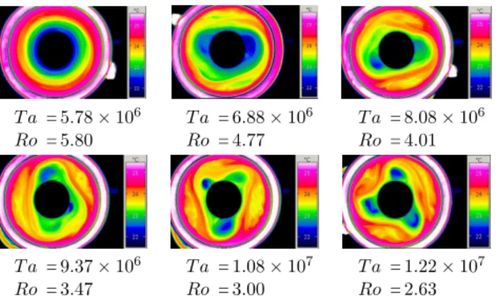
Fig. 6. Wide gap experiments. Pictures of the surface temperature
distribution for complex flow patterns in the first transition from axisymmetric flow (upper left panel) to wave mode of m=3 (bottom right panel). Cooled inner cylinder black, heated outer one pink to white, cold cells blue.
in part affected by small scale, spatially localized vortices which typically influenced only one wave lobe while the oth-ers remained unaffected. This parameter region is denoted as ‘transition to irregular flow’ in Fig. 4. However, at high ro-tation rates it was usually observed that the tracer particles were distributed randomly rather than followed the large-scale flow. Records of flow visualisation were used to de-termine the flow regime since they gave a much better im-pression of the actual flow state rather than the pictures. Due to this unexpected behaviour of the aluminium particles, the onset of the ‘irregular flow’ regime from visual inspection was somewhat a question of personal judgement.
The analysis of thermographic measurements generally agrees with the overall flow analysis from visualisation but also indicates some significant differences. Figure 6 gives an impression of the complex flow patterns found in the first transition where mode-interaction between mode 2 and 3 was observed by thermography at T a=8.08×10⁶ and T a=9.37×10⁶, which was also observed by flow visuali-sation, as was the non-unique flow state at T a=1.08×10⁷, where a mode competition between m=2 and m=3 was found to occur (Fig. 7). A breakdown of the wavy flow structure was observed several times, as shown in Fig. 7 at t =+600 s, and was found to be apparently non-periodic which must be subject to further analysis.
In contrast to the flow visualisation which indicated a steady flow of m=2 at T a=6.88×10⁶, here, thermographic measurements showed a wavy flow of m=2 which was slightly disturbed by a mode 3. We will discuss later that the complex vacillating flows found at the onset of the in-stability are supposably consistent with the 2/3I flow state which was characterised by Fr¨uh and Read (1997) in rigid lid experiments.
Thermographic measurements in the parameter range where ‘steady’ m=3 flows were observed by visualisation re-vealed a type of radial vacillation illustrated in Fig. 8 which shows a 150 s sequence of thermographic measurements. Cold cells separated from the inner wall, moved radially
out-t = 0 s t = +600 s t = +1200 s
t = +1800 s t = +2400 s t = +3000 s
1
Fig. 7. Wide gap experiments. Sequence of thermographic
mea-surements at T a=1.08×10⁷, Ro=3.00. t as time elapsed since the first frame in the figure.
t = 0 s t = +30 s t = +60 s
t = +90 s t = +120 s t = +150 s
1
Fig. 8. Wide gap experiments. Wavy flow of m=4 with radial
oscillation of the cold cells (T a=7.65×10⁷, Ro=0.41). t as time elapsed since the first frame in the figure. Note also the asymmetric formation of the wave lobes.
wards and then returned to the inner cylinder while their outer boundary remained unaffected. This type of radial os-cillation was first observed at T a=2.53×10⁷, Ro=1.25 and appeared regularly at higher rotation rates. Furthermore, an asymmetric formation of the wave lobes was observed which will be subject to the disussion in Sect. 4.
As such a vacillation of the wave shape is consistent with the definition of a structural vacillation, this range of Tay-lor number was reclassified as 3SV and 4SV , respectively. Together with the discrepancy at T a=6.88×10⁶, the regime diagram was revised as shown in Fig. 9.
3.2 Narrow gap experiments
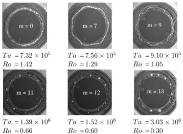
In narrow gap experiments, steady baroclinic waves up to m=13 but no complex flows were observed. Figure 10 shows the regime diagram determined by flow visualisation, and photographs of the surface flow, covering examples of differ-ent flow states, are displayed in Fig. 11. The transition to the wave flow regime, which was found to be affected by strong hysteresis, took place at T acrit=7.44×10⁵. Although the first transition remained unaffected by hysteresis, the minimum wave number was found to be unequal in case of increasing and decreasing Taylor numbers, respectively, i.e. mmin=5 for increasing T a and mmin=7 for decreasing T a. Furthermore, in case of decreasing Taylor numbers, no wavy flow of wave number 8 and 6 was observed.
1038 Th. von Larcher and C. Egbers: Experiments on transitions of baroclinic waves Tac= 6.33 × 10⁶ ↑ Tac 3 × 10⁶ 107 108 3 × 10⁸ Taylor number Ta
m=0
l2/3I
l .. .. .. .. .. .. .. .. .. .. .. .. .. .. .. .. .. .. .. .. .. .. .. .. . .. .. .. .. .. .. .. .. .. .. .. .. .. .. .. .. .. .. .. .. .. .. .. .. . .. .. .. .. .. .. .. .. .. .. .. .. .. .. .. .. .. .. .. .. .. .. .. .. . .. .. .. .. .. .. .. .. .. .. .. .. .. .. .. .. .. .. .. .. .. .. .. .. . .. .. .. .. .. .. .. .. .. .. .. .. .. .. .. .. .. .. .. .. .. .. .. .. . .. .. .. .. .. .. .. .. .. .. .. .. .. .. .. .. .. .. .. .. .. .. .. .. . .. .. .. .. .. .. .. .. .. .. .. .. .. .. .. .. .. .. .. .. .. .. .. .. . .. .. .. .. .. .. .. .. .. .. .. .. .. .. .. .. .. .. .. .. .. .. .. .. . .. .. .. .. .. .. .. .. .. .. .. .. .. .. .. .. .. .. .. .. .. .. .. .. . .. .. .. .. .. .. .. .. .. .. .. .. .. .. .. .. .. .. .. .. .. .. .. .. . .. .. .. .. .. .. .. .. .. .. .. .. .. .. .. .. .. .. .. .. .. .. .. .. . .. .. .. .. .. .. .. .. .. .. .. .. .. .. .. .. .. .. .. .. .. .. .. .. . .. .. .. .. .. .. .. .. .. .. .. .. .. .. .. .. .. .. .. .. .. .. .. .. . .. .. .. .. .. .. .. .. .. .. .. .. .. .. .. .. .. .. .. .. .. .. .. .. . .. .. .. .. .. .. .. .. .. .. .. .. .. .. .. .. .. .. .. .. .. .. .. .. . .. .. .. .. .. .. .. .. .. .. .. .. .. .. .. .. .. .. .. .. .. .. .. .. . .. .. .. .. .. .. .. .. .. .. .. .. .. .. .. .. .. .. .. .. .. .. .. .. . .. .. .. .. .. .. .. .. .. .. .. .. .. .. .. .. .. .. .. .. .. .. .. .. . .. .. .. .. .. .. .. .. .. .. .. .. .. .. .. .. .. .. .. .. .. .. .. .. . .. .. .. .. .. .. .. .. .. .. .. .. .. .. .. .. .. .. .. .. .. .. .. .. . .. .. .. .. .. .. .. .. .. .. .. .. .. .. .. .. .. .. .. .. .. .. .. .. . .. .. .. .. .. .. .. .. .. .. .. .. .. .. .. .. .. .. .. .. .. .. .. .. . .. .. .. .. .. .. .. .. .. .. .. .. .. .. .. .. .. .. .. .. .. .. .. .. . .. .. .. .. .. .. .. .. .. .. .. .. .. .. .. .. .. .. .. .. .. .. .. .. . .. .. .. .. .. .. .. .. .. .. .. .. .. .. .. .. .. .. .. .. .. .. .. .. . .. .. .. .. .. .. .. .. .. .. .. .. .. .. .. .. .. .. .. .. .. .. .. .. . .. .. .. .. .. .. .. .. .. .. .. .. .. .. .. .. .. .. .. .. .. .. .. .. . .. .. .. .. .. .. .. .. .. .. .. .. .. .. .. .. .. .. .. .. .. .. .. .. . .. .. .. .. .. .. .. .. .. .. .. .. .. .. .. .. .. .. .. .. .. .. .. .. . .. .. .. .. .. .. .. .. .. .. .. .. .. .. .. .. .. .. .. .. .. .. .. .. . .. .. .. .. .. .. .. .. .. .. .. .. .. .. .. .. .. .. .. .. .. .. .. .. . .. .. .. .. .. .. .. .. .. .. .. .. .. .. .. .. .. .. .. .. .. .. .. .. . .. .. .. .. .. .. .. .. .. .. .. .. .. .. .. .. .. .. .. .. .. .. .. .. . .. .. .. .. .. .. .. .. .. .. .. .. .. .. .. .. .. .. .. .. .. .. .. .. . ↑ ↓ transition to irregular flow as indicated by visualisation3
3 (SV)
4 (SV)
Fig. 9. Wide gap experiments, regime diagram as defined by
visu-alisation and thermography.
Tac= 7.44 × 10⁵ ↑ Tac 5 × 10⁵ 106 4 × 10⁶ Taylor number Ta
m=0
↑5
↑6
↑ ↓7
↑ ↓8
↑ ↓9
↑ ↓10
↑ .. .. .. .. .. .. .. .. .. .. .. .. .. .. .. .. .. .. .. .. .. .. .. .. .. .. .. .. .. .. .. .. .. .. .. .. .. .. .. .. .. .. .. .. . .. .. .. .. .. .. .. .. .. .. .. .. .. .. .. .. .. .. .. .. .. .. .. .. .. .. .. .. .. .. .. .. .. .. .. .. .. .. .. .. .. .. .. .. .. .. .. .. .. .. .. .. .. .. .. .. .. .. .. .. .. .. .. .. .. .. .. .. .. .. .. .. .. .. .. .. .. .. .. .. .. .. .. .. .. .. .. .. .. . .. .. .. .. .. .. .. .. .. .. .. .. .. .. .. .. .. .. .. .. .. .. .. .. .. .. .. .. .. .. .. .. .. .. .. .. .. .. .. .. .. .. .. .. .. .. .. .. .. .. .. .. .. .. .. .. .. .. .. .. .. .. .. .. .. .. .. .. .. .. .. .. .. .. .. .. .. .. .. .. .. .. .. .. .. .. .. .. .. . .. .. .. .. .. .. .. .. .. .. .. .. .. .. .. .. .. .. .. .. .. .. .. .. .. .. .. .. .. .. .. .. .. .. .. .. .. .. .. .. .. .. .. .. .. .. .. .. .. .. .. .. .. .. .. .. .. .. .. .. .. .. .. .. .. .. .. .. .. .. .. .. .. .. .. .. .. .. .. .. .. .. .. .. .. .. .. .. .. . .. .. .. .. .. .. .. .. .. .. .. .. .. .. .. .. .. .. .. .. .. .. .. .. .. .. .. .. .. .. .. .. .. .. .. .. .. .. .. .. .. .. .. .. .. .. .. .. .. .. .. .. .. .. .. .. .. .. .. .. .. .. .. .. .. .. .. .. .. .. .. .. .. .. .. .. .. .. .. .. .. .. .. .. .. .. .. .. .. . .. .. .. .. .. .. .. .. .. .. .. .. .. .. .. .. .. .. .. .. .. .. .. .. .. .. .. .. .. .. .. .. .. .. .. .. .. .. .. .. .. .. .. .. .. .. .. .. .. .. .. .. .. .. .. .. .. .. .. .. .. .. .. .. .. .. .. .. .. .. .. .. .. .. .. .. .. .. .. .. .. .. .. .. .. .. .. .. .. . .. .. .. .. .. .. .. .. .. .. .. .. .. .. .. .. .. .. .. .. .. .. .. .. .. .. .. .. .. .. .. .. .. .. .. .. .. .. .. .. .. .. .. .. .. .. .. .. .. .. .. .. .. .. .. .. .. .. .. .. .. .. .. .. .. .. .. .. .. .. .. .. .. .. .. .. .. .. .. .. .. .. .. .. .. .. .. .. .. . .. .. .. .. .. .. .. .. .. .. .. .. .. .. .. .. .. .. .. .. .. .. .. .. .. .. .. .. .. .. .. .. .. .. .. .. .. .. .. .. .. .. .. .. .. .. .. .. .. .. .. .. .. .. .. .. .. .. .. .. .. .. .. .. .. .. .. .. .. .. .. .. .. .. .. .. .. .. .. .. .. .. .. .. .. .. .. .. .. . .. .. .. .. .. .. .. .. .. .. .. .. .. .. .. .. .. .. .. .. .. .. .. .. .. .. .. .. .. .. .. .. .. .. .. .. .. .. .. .. .. .. .. .. .. .. .. .. .. .. .. .. .. .. .. .. .. .. .. .. .. .. .. .. .. .. .. .. .. .. .. .. .. .. .. .. .. .. .. .. .. .. .. .. .. .. .. .. .. . .. .. .. .. .. .. .. .. .. .. .. .. .. .. .. .. .. .. .. .. .. .. .. .. .. .. .. .. .. .. .. .. .. .. .. .. .. .. .. .. .. .. .. .. .. .. .. .. .. .. .. .. .. .. .. .. .. .. .. .. .. .. .. .. .. .. .. .. .. .. .. .. .. .. .. .. .. .. .. .. .. .. .. .. .. .. .. .. .. . .. .. .. .. .. .. .. .. .. .. .. .. .. .. .. .. .. .. .. .. .. .. .. .. .. .. .. .. .. .. .. .. .. .. .. .. .. .. .. .. .. .. .. .. .. .. .. .. .. .. .. .. .. .. .. .. .. .. .. .. .. .. .. .. .. .. .. .. .. .. .. .. .. .. .. .. .. .. .. .. .. .. .. .. .. .. .. .. .. . .. .. .. .. .. .. .. .. .. .. .. .. .. .. .. .. .. .. .. .. .. .. .. .. .. .. .. .. .. .. .. .. .. .. .. .. .. .. .. .. .. .. .. .. .. .. .. .. .. .. .. .. .. .. .. .. .. .. .. .. .. .. .. .. .. .. .. .. .. .. .. .. .. .. .. .. .. .. .. .. .. .. .. .. .. .. .. .. .. . .. .. .. .. .. .. .. .. .. .. .. .. .. .. .. .. .. .. .. .. .. .. .. .. .. .. .. .. .. .. .. .. .. .. .. .. .. .. .. .. .. .. .. .. .. .. .. .. .. .. .. .. .. .. .. .. .. .. .. .. .. .. .. .. .. .. .. .. .. .. .. .. .. .. .. .. .. .. .. .. .. .. .. .. .. .. .. .. .. . .. .. .. .. .. .. .. .. .. .. .. .. .. .. .. .. .. .. .. .. .. .. .. .. .. .. .. .. .. .. .. .. .. .. .. .. .. .. .. .. .. .. .. .. .. .. .. .. .. .. .. .. .. .. .. .. .. .. .. .. .. .. .. .. .. .. .. .. .. .. .. .. .. .. .. .. .. .. .. .. .. .. .. .. .. .. .. .. .. . .. .. .. .. .. .. .. .. .. .. .. .. .. .. .. .. .. .. .. .. .. .. .. .. .. .. .. .. .. .. .. .. .. .. .. .. .. .. .. .. .. .. .. .. .. .. .. .. .. .. .. .. .. .. .. .. .. .. .. .. .. .. .. .. .. .. .. .. .. .. .. .. .. .. .. .. .. .. .. .. .. .. .. .. .. .. .. .. .. . .. .. .. .. .. .. .. .. .. .. .. .. .. .. .. .. .. .. .. .. .. .. .. .. .. .. .. .. .. .. .. .. .. .. .. .. .. .. .. .. .. .. .. .. .. .. .. .. .. .. .. .. .. .. .. .. .. .. .. .. .. .. .. .. .. .. .. .. .. .. .. .. .. .. .. .. .. .. .. .. .. .. .. .. .. .. .. .. .. . .. .. .. .. .. .. .. .. .. .. .. .. .. .. .. .. .. .. .. .. .. .. .. .. .. .. .. .. .. .. .. .. .. .. .. .. .. .. .. .. .. .. .. .. .. .. .. .. .. .. .. .. .. .. .. .. .. .. .. .. .. .. .. .. .. .. .. .. .. .. .. .. .. .. .. .. .. .. .. .. .. .. .. .. .. .. .. .. .. . .. .. .. .. .. .. .. .. .. .. .. .. .. .. .. .. .. .. .. .. .. .. .. .. .. .. .. .. .. .. .. .. .. .. .. .. .. .. .. .. .. .. .. .. .. .. .. .. .. .. .. .. .. .. .. .. .. .. .. .. .. .. .. .. .. .. .. .. .. .. .. .. .. .. .. .. .. .. .. .. .. .. .. .. .. .. .. .. .. . .. .. .. .. .. .. .. .. .. .. .. .. .. .. .. .. .. .. .. .. .. .. .. .. .. .. .. .. .. .. .. .. .. .. .. .. .. .. .. .. .. .. .. .. .. .. .. .. .. .. .. .. .. .. .. .. .. .. .. .. .. .. .. .. .. .. .. .. .. .. .. .. .. .. .. .. .. .. .. .. .. .. .. .. .. .. .. .. .. . .. .. .. .. .. .. .. .. .. .. .. .. .. .. .. .. .. .. .. .. .. .. .. .. .. .. .. .. .. .. .. .. .. .. .. .. .. .. .. .. .. .. .. .. .. .. .. .. .. .. .. .. .. .. .. .. .. .. .. .. .. .. .. .. .. .. .. .. .. .. .. .. .. .. .. .. .. .. .. .. .. .. .. .. .. .. .. .. .. . .. .. .. .. .. .. .. .. .. .. .. .. .. .. .. .. .. .. .. .. .. .. .. .. .. .. .. .. .. .. .. .. .. .. .. .. .. .. .. .. .. .. .. .. .. .. .. .. .. .. .. .. .. .. .. .. .. .. .. .. .. .. .. .. .. .. .. .. .. .. .. .. .. .. .. .. .. .. .. .. .. .. .. .. .. .. .. .. .. . .. .. .. .. .. .. .. .. .. .. .. .. .. .. .. .. .. .. .. .. .. .. .. .. .. .. .. .. .. .. .. .. .. .. .. .. .. .. .. .. .. .. .. .. .. .. .. .. .. .. .. .. .. .. .. .. .. .. .. .. .. .. .. .. .. .. .. .. .. .. .. .. .. .. .. .. .. .. .. .. .. .. .. .. .. .. .. .. .. . .. .. .. .. .. .. .. .. .. .. .. .. .. .. .. .. .. .. .. .. .. .. .. .. .. .. .. .. .. .. .. .. .. .. .. .. .. .. .. .. .. .. .. .. .. .. .. .. .. .. .. .. .. .. .. .. .. .. .. .. .. .. .. .. .. .. .. .. .. .. .. .. .. .. .. .. .. .. .. .. .. .. .. .. .. .. .. .. .. . .. .. .. .. .. .. .. .. .. .. .. .. .. .. .. .. .. .. .. .. .. .. .. .. .. .. .. .. .. .. .. .. .. .. .. .. .. .. .. .. .. .. .. .. .. .. .. .. .. .. .. .. .. .. .. .. .. .. .. .. .. .. .. .. .. .. .. .. .. .. .. .. .. .. .. .. .. .. .. .. .. .. .. .. .. .. .. .. .. . .. .. .. .. .. .. .. .. .. .. .. .. .. .. .. .. .. .. .. .. .. .. .. .. .. .. .. .. .. .. .. .. .. .. .. .. .. .. .. .. .. .. .. .. .. .. .. .. .. .. .. .. .. .. .. .. .. .. .. .. .. .. .. .. .. .. .. .. .. .. .. .. .. .. .. .. .. .. .. .. .. .. .. .. .. .. .. .. .. . .. .. .. .. .. .. .. .. .. .. .. .. .. .. .. .. .. .. .. .. .. .. .. .. .. .. .. .. .. .. .. .. .. .. .. .. .. .. .. .. .. .. .. .. .. .. .. .. .. .. .. .. .. .. .. .. .. .. .. .. .. .. .. .. .. .. .. .. .. .. .. .. .. .. .. .. .. .. .. .. .. .. .. .. .. .. .. .. .. . .. .. .. .. .. .. .. .. .. .. .. .. .. .. .. .. .. .. .. .. .. .. .. .. .. .. .. .. .. .. .. .. .. .. .. .. .. .. .. .. .. .. .. .. .. .. .. .. .. .. .. .. .. .. .. .. .. .. .. .. .. .. .. .. .. .. .. .. .. .. .. .. .. .. .. .. .. .. .. .. .. .. .. .. .. .. .. .. .. . .. .. .. .. .. .. .. .. .. .. .. .. .. .. .. .. .. .. .. .. .. .. .. .. .. .. .. .. .. .. .. .. .. .. .. .. .. .. .. .. .. .. .. .. .. .. .. .. .. .. .. .. .. .. .. .. .. .. .. .. .. .. .. .. .. .. .. .. .. .. .. .. .. .. .. .. .. .. .. .. .. .. .. .. .. .. .. .. .. . .. .. .. .. .. .. .. .. .. .. .. .. .. .. .. .. .. .. .. .. .. .. .. .. .. .. .. .. .. .. .. .. .. .. .. .. .. .. .. .. .. .. .. .. .. .. .. .. .. .. .. .. .. .. .. .. .. .. .. .. .. .. .. .. .. .. .. .. .. .. .. .. .. .. .. .. .. .. .. .. .. .. .. .. .. .. .. .. .. . .. .. .. .. .. .. .. .. .. .. .. .. .. .. .. .. .. .. .. .. .. .. .. .. .. .. .. .. .. .. .. .. .. .. .. .. .. .. .. .. .. .. .. .. .. .. .. .. .. .. .. .. .. .. .. .. .. .. .. .. .. .. .. .. .. .. .. .. .. .. .. .. .. .. .. .. .. .. .. .. .. .. .. .. .. .. .. .. .. . .. .. .. .. .. .. .. .. .. .. .. .. .. .. .. .. .. .. .. .. .. .. .. .. .. .. .. .. .. .. .. .. .. .. .. .. .. .. .. .. .. .. .. .. .. .. .. .. .. .. .. .. .. .. .. .. .. .. .. .. .. .. .. .. .. .. .. .. .. .. .. .. .. .. .. .. .. .. .. .. .. .. .. .. .. .. .. .. .. . .. .. .. .. .. .. .. .. .. .. .. .. .. .. .. .. .. .. .. .. .. .. .. .. .. .. .. .. .. .. .. .. .. .. .. .. .. .. .. .. .. .. .. .. .. .. .. .. .. .. .. .. .. .. .. .. .. .. .. .. .. .. .. .. .. .. .. .. .. .. .. .. .. .. .. .. .. .. .. .. .. .. .. .. .. .. .. .. .. . .. .. .. .. .. .. .. .. .. .. .. .. .. .. .. .. .. .. .. .. .. .. .. .. .. .. .. .. .. .. .. .. .. .. .. .. .. .. .. .. .. .. .. .. .. .. .. .. .. .. .. .. .. .. .. .. .. .. .. .. .. .. .. .. .. .. .. .. .. .. .. .. .. .. .. .. .. .. .. .. .. .. .. .. .. .. .. .. .. . .. .. .. .. .. .. .. .. .. .. .. .. .. .. .. .. .. .. .. .. .. .. .. .. .. .. .. .. .. .. .. .. .. .. .. .. .. .. .. .. .. .. .. .. .. .. .. .. .. .. .. .. .. .. .. .. .. .. .. .. .. .. .. .. .. .. .. .. .. .. .. .. .. .. .. .. .. .. .. .. .. .. .. .. .. .. .. .. .. . .. .. .. .. .. .. .. .. .. .. .. .. .. .. .. .. .. .. .. .. .. .. .. .. .. .. .. .. .. .. .. .. .. .. .. .. .. .. .. .. .. .. .. .. .. ↓11
↑ ↓12
13
indirect detection of wave patternFig. 10. Narrow gap experiments, regime diagram as defined by
flow visualisation.
It has to be kept in mind that the extent of each wave num-ber is only the documented extent on following the bifurca-tion sequence either from axisymmetric flow or from the high wave number 13. Wave numbers 6 and 8 existed probably to lower values of Taylor number than indicated in Fig. 10 since the experiment did not trace each wave number in the decreasing Taylor number direction but started at the higher wave number and followed therefore only the highest possi-ble wave number.
With increasing Taylor numbers, the tracer particles were more and more accumulated in the outer vortices (cf. Fig. 11) and finally, at comparatively high rotation rates, the jet-stream could be hardly identified. Here, assuming that each accumulation marks an outer vortex with the jet-stream on the inner side, which was observed at moderate rotation rates, we could infer the wave number of the flow indirectly. While this estimate of the wave number is open to criticism, there was no indication of a transition to a qualitatively different flow regime, such as to irregular flows. However, other ob-servation techniques would have to be applied in future to determine the spatial and temporal structure of the flows re-liably. T a = 7.32 × 10⁵ Ro = 1.42 T a = 7.56 × 10⁵ Ro = 1.29 T a = 9.10 × 10⁵ Ro = 1.05 T a = 1.39 × 10⁶ Ro = 0.66 T a = 1.52 × 10⁶ Ro = 0.60 T a = 3.03 × 10⁶ Ro = 0.30 1
Fig. 11. Narrow gap experiments, photographs of different flow
states. Note the accumulation of the aluminium tracers at higher Taylor numbers.
4 Discussion
Series of flow visualisations and temperature measurements of the surface flow in a rotating differentially heated annu-lus with a free surface and a flat bottom topography were presented using two different radius ratios. In wide gap ex-priments, the application of various measurement techniques revealed some surprising differences that might partly caused by the techniques themselves. Some regions of vacillating flows were uncovered by thermography whereas flow vi-sualisation indicated steady flow pattern. Furthermore, an asymmetric formation of the jet-stream structure which is ap-parently associated with radial oscillations of the cold cells was observed by thermography but not by flow visualisation at moderate and higher Taylor numbers. Due to the non-rotation of the heat sensitive camera, one has to take into ac-count that some of the thermographic recordings, especially at high Taylor numbers, could be affected by blurring effects, or similar, due to technical reasons. Nevertheless, since the quality of the records was subject to careful inspections using two reference targets with different temperatures which were co-rotated during the temperature measurements, the asym-metric distribution of the cold cells is evident, as is the radial oscillation of the wavy flow. However, since the spacious jet-stream was not affected by this in a significant manner and due to the fact that the tracer particles followed the dom-inating large-scale flow it could be accepted that the zonal displacement of the cold cells is barely perceptible in flow visualisation.
Two different types of complex flows were found in wide gap experiments. While the flow was dominated by m=2 mode and only weak influenced by mode 3 at the onset of the first transition, the m=2 flow was more and more affected by the m=3 mode with increasing Taylor number. As the anal-ysis of thermographic measurements indicates, that flow pat-terns might be identified as a superposition of two coexisting
waves with different zonal wave numbers and phase speeds, denoted as ‘interference vacillation’ (I V ), which was found to occur in experiments with a free surface (e.g. Pfeffer and Fowlis, 1968; Kaiser, 1970) as in rigid lid experiments (Fr¨uh and Read (1997)).
Numerical studies using two-layer models have shown that such mixed-mode flow states can only be stable when the β-effect is considered, (e.g. Hart, 1981; Pedlosky, 1981; Moroz and Holmes, 1984; Mansbridge, 1984). Since we focussed on experiments with a free surface, the surface was affected by the centrifugal force and had a parabolic profile, i.e. a β-plane, but on the other hand due to relative low rotation rates in the parameter range of the complex flows this might not had a strong effect. Fr¨uh and Read (1997) discussed the sta-bilizing effect of I V flows following an approach by Ohlsen and Hart (1989a) and Ohlsen and Hart (1989b), resp., who observed a type of nonlinear interference vacillation in which a string of triads and self interactions could drive the I V flow. They were able to prove the fullfilment of the so-called har-monic triad conditions in their experiments for the classified 2+3I V mode and concluded that, even in a f -plane flow, I V flows are possible and stable with harmonic interactions and self interactions only, i.e. the flow is driven through wave-wave interactions.
Just before the onset of the steady wave flow of m=3 an-other type of complex vacillating flow was observed. The m=3 mode collapses and is replaced by a I V flow pattern of 2 and 3. The m=3 mode is then recovered and collapses again. This flow behaviour is typically described by ‘inter-mittent bursting’ but here the flow might also be comparable to a m=2−3A flow pattern, as observed by Fr¨uh and Read (1997), where the dominant wave number alternates between wave number 2 and 3. In this case, the flow may be forced through wave-zonal flow interactions. However, regarding our experiments, an explicit characterisation of the flow dy-namics at this critical parameter points can hardly be done by visualisation and thermography only and must be subject to further investigations.
The complex vacillation involving two adjacent zonal wave numbers appears to preclude the possibility of hys-teresis. This may be due to the fact that the two modes do not form separate basins of attraction as described by Fr¨uh and Read (1997) who observed this behaviour in the rigid lid case. Regarding the possibility of a 2−3A mode, a attrac-tor switching could be caused for example by a crisis where two potential attractor shells clash as described by e.g. Gre-bogi et al. (1987) and Fr¨uh and Read (1997). Furthermore, stochastic fluctuations could also be responsible, denoted as noise-induced crisis, which is discussed by Fr¨uh and Read (1997) to cause the 2−3A flow in their experiments.
Unlike exclusion of hysteresis in the first transition zone, vacillating flows at higher Taylor numbers do allow for mod-erate hysteresis. From the thermography it appears that this vacillation involved a radial oscillation of temperature min-ima. This could be consistent with an oscillation of a higher radial mode of the same azimuthal wave as observed in ex-periments by Pfeffer et al. (1980) and theoretically by Weng
et al. (1986) whose numerical study, using truncated spectral Eady models with two Ekman layers of different strength, show the existence of a quasi-periodic vacillating flow with two different radial modes of the same azimuthal wave num-ber.
It was a surprise that the radial oscillations of the m=3 and m=4 pattern were not observed in flow visualisation but only by thermography. While the vacillating flows at the onset of the first instability might be in part too weak to be identi-fied by visual inspection, which then would be a human fac-tor more than a technical one, the radial vacillations are too strong to be overlooked in flow visualisation. An explana-tion might be that the aluminium particles are captured in the dominating wavy flow structure and are therefore not able to follow the relative rapid change in radial direction which is in addition only significant at the inner cylinder side of the cold vortices and thus outside the jet-stream flow. This possibility is also supported by the fact that the overall jet-stream struc-ture is not influenced by the radial oscillation as indicated by the thermography.
Narrow gap experiments were done with visual inspection of the surface flow only. Steady flows up to wave number 13 were detected, partly by an indirect estimate of the wave mode. Due to the accumulation of the tracer particles vi-sual inspection was not possible any longer at high rotation rates and the experiments were restricted to Taylor numbers lower than 4×10⁶. As described in Sect. 3.2, waves with wave number 6 and 8 were missed when the rotation rate was decreased. Due to the limited number of runs which had been done for the narrow gap case, and as an additional ar-gument to the discussion in Sect. 3.2, we also can not rule out the possibility that stochastic fluctuations, as mentioned above, were responsible for the absence of the wave numbers which should then be observed in supplemental experiments. As the wide gap experiments have shown, flow visuali-sation may not be sufficient to analyse the flow regimes in detail. However, due to the restricition of the narrow gap in radial direction the appearance of only ‘steady’ flows might be possible. Furthermore, strong hysteresis affected the flow in the narrow gap. Regarding the discussion above where the vacillation of adjacent modes may preclude hysteresis, it might be possible, that hysteresis is linked with the occur-rence of steady waves and precludes vacillating flows. All in all, the classification of ‘steady’ waves in the regime diagram for the narrow gap case on the basis of flow visualisation only can be accepted with reservation. Even though complex vac-illating flows were not observed in the narrow gap case we can not rule out that the clustering of particles mark the on-set of some type of SV -like flows.
Recent work has shown that inertia-gravity waves can be generated by baroclinic waves in the laboratory (Williams et al. (2005), see references therein for possible inertia-gravity wave generation mechanisms), and that the inertia-gravity waves may exert a strong influence on baroclinic wave tran-sitions (Williams et al. (2004)). Also Read (1992) mentioned the existence of gravity waves in the baroclinic annulus of fluid as he analysed bursting oscillations, weak in amplitude,
1040 Th. von Larcher and C. Egbers: Experiments on transitions of baroclinic waves which he had observed in experiments. Due to technical
rea-sons Read could not rule out the possibility that these oscil-lations arose from interactions with the experimental setup rather than were generated by internal dynamics of the fluid. However, there is no evidence of gravity waves in our ex-periments, which should be detected by thermographic mea-surements due to the high quality heat sensitive camera, if possible.
5 Conclusions
Our experiments uncovered a variety of complex flow regimes and a limited ‘steady’ wave regime in the wide gap case. The vacillating flows are comparable with types of complex vacillating flows found by Fr¨uh and Read (1997) even though they used a fluid with P r=26.7 in an appa-ratus with a rigid lid and a different aspect ratio. Our re-sults might be in contrast to some extent to studies by Jonas (1981) and Pfeffer et al. (1980) who found that vacillating wave regimes are broadened in higher Prandtl number fluids where the steady wave regime is then limited. Experiments of Sitte and Egbers (2000), who determined flow regimes by flow visualisation and, particularly, through nonlinear time series analysis of velocity data, using a free surface appara-tus with an aspect ratio of 4.4 and a moderate Prandtl number fluid of P r=7, may also confirm this since they found a lim-ited region of complex oscillating flows at the onset of the first instability as well as an extended region of steady waves with different wave number and strong hysteresis. On the other hand, Sitte and Egbers (2000) determined an extended region of distorted flows at moderate to higher Taylor num-bers, denoted as SV therein, in which structural fluctuations were increased with the rotation rate. They assumed this re-gion as the transition to turbulent flow. It is speculative that radial oscillations as observed in our experiments were (in part) also responsible for some flow states in the SV regime of Sitte and Egbers (2000).
Our wide gap experiments show that vacillation and hys-teresis are only compatible if the vacillation does not involve adjacent wave numbers which is also observed by Fr¨uh and Read (1997) in rigid lid experiments. Narrow gap experi-ments show much stronger hysteresis than observed in the wide channel case. This may be due to the higher azimuthal wave number and restriction of radial modes. However, since flow visualisations appear to be unreliable to pick up any-thing other than strong oscillations further experiments are necessary to identify temporal and spatial structures of the flow in the narrow gap.
Since the early eighties, different approaches to dynami-cal systems analysis were proposed, in particular the ‘method of delays’ (MOD) by Takens (1981) and the ‘singular sys-tems analysis’ (SSA) by Broomhead and King (1986) that was extended to the ‘multivariate singular systems analysis’ (M − SSA) which was implemented by Read (1993). Both methods were successfully applied in experimental fluid dy-namics, e.g. Buzug (1994) and Wulf et al. (1999), both of
them charaterised the dynamics of complex spherical Cou-ette flows using the MOD, as it was also used by Sitte and Egbers (2000), and by Read (1992) and Read (1993) who used the SSA and M−SSA, resp., to investigate the dynam-ics of complex flows in the baroclinic annulus. We have mea-sured velocity time series data up to several hours not only in the complex flow regimes but also in the ‘steady’ wave regime using the optical Laser Doppler Velocimetry. The evaluation of the complex flow dynamics of the observed wide gap flows from this data is the aim of further work.
Acknowledgements. The authors thank W.-G. Fr¨uh for his
encour-agement, support and fruitful discussions during this work and P. Williams for his helpful comments. This study was in great parts funded by the Deutsche Forschungsgemeinschaft (DFG).
Edited by: J.-B. Flor
Reviewed by: W.-G. Fr¨uh and P. Willams
References
Broomhead, D. S. and King, G. P.: Extracting qualitative dynamics from experimental data, Physica D, 20, 217–236, 1986. Buzug, T.: Analyse chaotischer Systeme, BI-Wiss.-Verl.,
Mannheim (u.a.), 1994.
Cole, R. J.: Hysteresis effects in a differentially heated rotating fluid annulus, Quart. J. Roy. Meteor. Soc., 97, 506–518, 1971. Fein, J. S. and Pfeffer, R. L.: An experimental study of the effects of
Prandtl number on thermal convection in a rotating, differentially heated cylindrical annulus of fluid, J. Fluid Mech., 75, 81–112, 1976.
Fowlis, W. W. and Hide, R.: Thermal convection in a rotating an-nulus of liquid: effect of viscosity on the transition between ax-isymmetric and non–axax-isymmetric flow regimes, J. Atmos. Sci-ences, 22, 541–558, 1965.
Fr¨uh, W.-G. and Read, P. L.: Wave interactions and the transition to chaos of baroclinic waves in a thermally driven rotating annulus, Phil. Trans. R. Soc. Lond. A, 355, 101–153, 1997.
Fultz, D.: Development in Controlled Experiments on Larger Scale Geophysical Problems, Adv. Geophys., 7, 1–104, Academic Press, 1961.
Fultz, D., Long, R. R., Owens, G. V., Bohan, W., Kaylor, R., and Weil, J.: Studies of thermal convection in a rotating cylinder with some implications for large-scale atmospheric motions, Meteor. Monogr., 4, 1–104, Amer. Meteor. Soc., 1959.
Grebogi, C., Ott, E., Romeiras, F., and Yorke, J. A.: Critical expo-nents for crisis-induced intermittency, Phys. Rev. A, 36, 5365– 5380, 1987.
Guckenheimer, J.: Dimension Measurements for Geostrophic Tur-bulence, Phys. Rev. Lett., 51, 1438–1441, 1983.
Hart, J. E.: Wavenumber selection in nonlinear baroclinic instabil-ity, J. Atmos. Sci., 38, 400–408, 1981.
Hide, R.: An experimental study of thermal convection in a rotating fluid, Phil. Trans. Roy. Soc. Lond. A, 250, 441–478, 1958. Hide, R. and Mason, P. J.: Baroclinic waves in a rotating fluid
sub-ject to internal heating, Phil. Trans. Roy. Soc. Lond. A, 268, 201– 232, 1970.
Hide, R. and Mason, P. J.: Sloping convection in a rotating fluid, Adv. in Phys., 24, 47–99, 1975.
Hignett, P., White, A. A., Carter, R. D., Jackson, W. D., and Small, R. M.: A comparison of laboratory measurements and
numeri-cal simulations of baroclinic wave flows in a rotating cylindrinumeri-cal annulus, Quart. J. Roy. Meteor. Soc., 111, 131–154, 1985. Jonas, P. R.: Some effects of boundary conditions and fluid
proper-ties on vacillation in thermally driven rotating flow in an annulus, Geophys. Astrophys. Fluid Dyn., 18, 1–23, 1981.
Kaiser, J. A. C.: Rotating deep annulus convection 2. Wave insta-bilities, vertical stratification and associated theories, Tellus, 22, 275–287, 1970.
Lewis, G. M. and Nagata, W.: Linear stability analysis for the dif-ferentially heated rotating annulus, Geophys. Astrophys. Fluid Dyn., 98, 279–299, 2004.
Lorenz, E. N.: Simplified dynamic equations applied to the rotating-basin experiments, J. Atmos. Sciences, 19, 39–51, 1962. Mansbridge, J. V.: Wavenumber transition in baroclinically
unsta-ble flows, J. Atmos. Sci., 41, 925–930, 1984.
Miller, T. L. and Butler, K. A.: Hysteresis and the Transition be-tween Axisymmetric Flow and Wave Flow in the Baroclinic An-nulus, J. Atmos. Sci., 48, 811–823, 1991.
Miller, T. L. and Gall, R. L.: A linear analysis of the transition curve for the baroclinic annulus, J. Atmos. Sci., 40, 2293–2303, 1983. Moroz, M. D. and Holmes, P.: Double Hopf bifurcation and quasi-periodic flow in a model for baroclinic instability, J. Atmos. Sci., 41, 3147–3160, 1984.
Ohlsen, D. R. and Hart, J. E.: Transitions to baroclinic chaos on a
β-plane, J. Fluid Mech., 203, 23–50, 1989a.
Ohlsen, D. R. and Hart, J. E.: Nonlinear interference vacillations, Geophys. Astrophys. Fluid Dyn., 45, 213–235, 1989b.
Pedlosky, J.: The nonlinear dynamics of baroclinic wave ensembles, J. Fluid Mech., 102, 169–209, 1981.
Pfeffer, R. L. and Fowlis, W. W.: Wave dispersion in a rotating differentially heated cylindrical annulus of fluid, J. Atmos. Sci., 25, 361–371, 1968.
Pfeffer, R. L., Buzyna, G., and Kung, R.: Time-dependent modes of thermally driven rotating fluids, J. Atmos. Sci., 37, 2129–2149, 1980.
Read, P. L.: Applications of singular systems analysis to “Baro-clinic chaos”, Physica D, 58, 455–468, 1992.
Read, P. L.: Phase portrait reconstruction using multivariate singu-lar systems analysis, Physica D, 69, 353–365, 1993.
Read, P. L., Bell, M. J., Johnson, D. W., and Small, R. M.: Quasi-periodic and chaotic flow regimes in a thermaly-driven, rotating fluid annulus, J. Fluid Mech., 238, 599–632, 1992.
Sitte, B. and Egbers, C.: Higher order dynamics of baroclinc waves, in: Physics of Rotating Fluids (Proc. 11th Int. Couette-Taylor Workshop, 20–23 July 1999, Bremen, Germany), edited by: Pfis-ter, G. and Egbers, C., vol. 549 of Lecture Notes in Physics, Springer, Berlin, 2000.
Takens, F.: Detecting strange attractors in turbulence, in: Dynami-cal Systems and Turbulence, edited by: Rand, D. A. and Young, L. S., vol. 898 of Lecture Notes in Mathematics, pp. 366–381, Springer, Berlin, 1981.
von Larcher, T. and Egbers, C.: Dynamics of baroclinic instabili-ties using methods of nonlinear time series analysis, in: Progress in Turbulence, edited by: Peinke, J., Kittel, A., Barth, S., and Oberlack, M., Springer, Berlin, 2005.
Weng, H.-Y., Barcilon, A., and Magnan, J.: Transitions between baroclinic flow regimes, J. Atm. Sci., 43, 1760–1777, 1986. Williams, P. D., Haine, T. W. N., and Read, P. L.: Stochastic
res-onance in a nonlinear model of a rotating, stratified shear flow, with a simple stochastic inertia-gravity wave parameterization, Nonlin. Processes Geophys., 11, 127–135, 2004,
SRef-ID: 1607-7946/npg/2004-11-127.
Williams, P. D., Haine, T. W. N., and Read, P. L.: On the generation mechanisms of short-scale unbalanced modes in rotating two-layer flows with vertical shear, J. Fluid Mech., 528, 1–22, 2005. Wulf, P., Egbers, C., and Rath, H. J.: Routes to chaos in wide-gap