HAL Id: insu-01983139
https://hal-insu.archives-ouvertes.fr/insu-01983139
Submitted on 16 Jan 2019
HAL is a multi-disciplinary open access
archive for the deposit and dissemination of
sci-entific research documents, whether they are
pub-lished or not. The documents may come from
teaching and research institutions in France or
abroad, or from public or private research centers.
L’archive ouverte pluridisciplinaire HAL, est
destinée au dépôt et à la diffusion de documents
scientifiques de niveau recherche, publiés ou non,
émanant des établissements d’enseignement et de
recherche français ou étrangers, des laboratoires
publics ou privés.
Thibault Duretz, Alban Souche, Rene de Borst, Laetitia Le Pourhiet
To cite this version:
Thibault Duretz, Alban Souche, Rene de Borst, Laetitia Le Pourhiet.
The Benefits of Using
a Consistent Tangent Operator for Viscoelastoplastic Computations in Geodynamics.
Geochem-istry, Geophysics, Geosystems, AGU and the Geochemical Society, 2018, 19 (12), pp.4904-4924.
�10.1029/2018gc007877�. �insu-01983139�
The Benefits of Using a Consistent Tangent Operator for
Viscoelastoplastic Computations in Geodynamics
Thibault Duretz1,2 , Alban Souche3,4, René de Borst5 , and Laetitia Le Pourhiet6
1Univ Rennes, CNRS, Géosciences Rennes UMR 6118, Rennes, France,2Institut des Sciences de la Terre, University of
Lausanne, Lausanne, Switzerland,3Physics of Geological Processes, The NJORD Center, Geosciences Department,
University of Oslo, Oslo, Norway,4Computational Physiology, Simula Research Laboratory, Lysaker, Norway,5Department of Civil and Structural Engineering, University of Sheffield, Sheffield, UK,6CNRS-INSU, Institut des Sciences de la Terre Paris,
ISTeP UMR 7193, Sorbonne Université, Paris, France
Abstract
Strain localization is ubiquitous in geodynamics and occurs at all scales within the lithosphere. How the lithosphere accommodates deformation controls, for example, the structure of orogenic belts and the architecture of rifted margins. Understanding and predicting strain localization is therefore of major importance in geodynamics. While the deeper parts of the lithosphere effectively deform in a viscous manner, shallower levels are characterized by an elastoplastic rheological behavior. Herein we propose a fast and accurate way of solving problems that involve elastoplastic deformations based on the consistent linearization of the time-discretized elastoplastic relation and the finite difference method. The models currently account for the pressure-insensitive Von Mises and the pressure-dependent Drucker-Prager yield criteria. Consistent linearization allows for resolving strain localization at kilometer scale while providing optimal, that is, quadratic convergence of the force residual. We have validated our approach by a qualitative and quantitative comparison with results obtained using an independent code based on the finite element method. We also provide a consistent linearization for a viscoelastoplastic framework, and we demonstrate its ability to deliver exact partitioning between the viscous, the elastic, and the plastic strain components. The results of the study are fully reproducible, and the codes are available as a subset of M2Di MATLAB routines.1. Introduction
The deformation of the lithosphere is classically divided into brittle and ductile regimes (Fossen, 2016). The brittle regime describes processes that are best modeled by frictional slip along discrete slip planes (disloca-tions or faults) in an elastic medium, while in the ductile regime, processes are best described by distributed strains within the framework of continuum mechanics. The emergence of localized deformations at the scale of the lithosphere can ultimately lead to the fragmentation of continents, the individualization of tectonic plates, and the formation of plate boundaries. Such a process lasts typically for millions of years and results in hundreds of kilometers of displacements. At that scale, faults are not planes anymore but rather shear zones, involving many slip planes, which are better approximated by continuum mechanics rather than fractured mechanics.
At the scale of thin sections, rock deformation is typically accommodated by mechanisms such as crystal plas-ticity and brittle fracturing (Passchier & Trouw, 1996). Crystal plasplas-ticity is typical of the so-called ductile regime and results in macroscopic viscous creep, which implies a rate dependence with often a non-Newtonian behavior. Brittle fracturing induces the formation of gouges or damaged zones and results in macroscopic frictional plastic behavior, which implies pressure dependence. The transition from viscous creep to frictional plastic behavior is primarily controlled by the confining pressure and the temperature (Evans et al., 1990). Temperature and pressure have competing effects on the strength of rocks, and as both increase with depth in the lithosphere, so-called brittle-ductile transition zones arise. Elastic deformations in the lithosphere are small and are often neglected in the study of long-term tectonic processes.
Quantification of tectonic processes relies on establishing quantitative models in an analytical, experimen-tal (analog), or numerical form. While analytical modeling can provide first-order insights into the physics of tectonic processes, it is often limited to small deformations. Experimental modeling enables to study large
TECHNICAL
REPORTS:
METHODS
10.1029/2018GC007877 Key Points: • Pressure-dependent plasticity converges with elastoplastic and viscoelastoplastic rheology • We provide fast and concise MATLABsource codes for full reproducibility • We combined consistent tangent
linearization together with finite difference method
Correspondence to:
T. Duretz,
Citation:
Duretz, T., Souche, A., de Borst, R., & Le Pourhiet, L. (2018). The benefits of using a consistent tangent operator for viscoelastoplastic computations in geodynamics. Geochemistry, Geophysics, Geosystems, 19, 4904–4924. https://doi.org/10.1029/2018GC007877 Received 1 AUG 2018 Accepted 13 NOV 2018
Accepted article online 15 NOV 2018 Published online 13 DEC 2018
©2018. The Authors.
This is an open access article under the terms of the Creative Commons Attribution-NonCommercial-NoDerivs License, which permits use and distribution in any medium, provided the original work is properly cited, the use is non-commercial and no modifications or adaptations are made.
displacements in three dimensions and can account for both frictional plastic (using sand) and linear viscous rheologies (using, e.g., silicon putty and honey). Yet plate formation and deformation involve processes that are beyond the scope of this approach (e.g., thermomechanical coupling, non-Newtonian creep, and multi-physics couplings). For these reasons numerical simulations are slowly taking over the lead for simulating the formation and the evolution of tectonic plates.
In numerical geodynamic modeling, the treatment of linear and non-Newtonian viscous creep can be con-sidered as part of the state of the art. However, the implementation of plastic frictional laws to simulate faults and enhance strain localization can be problematic for numerical codes aimed at modeling long-term tecton-ics processes. Numerical modeling of frictional plastic deformation has therefore recently received significant attention within the long-term tectonic community (Buiter et al., 2006; Buiter et al., 2016; Choi & Petersen, 2015; Olive et al., 2016).
Numerical modeling based on an engineering solid mechanics approach, assuming small displacement gradi-ents, has been widely used in geosciences since the early 1990s when Fast Lagrangian Analysis of Continuum (FLAC) (Cundall, 1989) was reimplemented into a noncommercial code, in two-dimensional (2-D) (Poliakov & Podladchikov, 1992), and, later, in 3-D (Choi et al., 2008). The explicit time-stepping strategy was, at the time, not competitive with the large time steps that could be achieved using implicit approaches based on incompressible viscous flow or Stokes equations (Fullsack, 1995; Gerya & Yuen, 2003; Kaus, 2010; Moresi et al., 2007).
Within incompressible viscous flow formulations, plasticity is generally implemented in a viscoplasticity fash-ion, following the original work of Willett (1992). The value of viscosity is adapted in order to locally satisfy the yield condition in the regions where plastic yielding occurs. In order to satisfy global equilibrium (i.e., force bal-ance), this approach needs to be complemented with global nonlinear iterations. The viscoplastic approach is often used together with Picard-type iterations (Kaus, 2010; Moresi et al., 2007) which results in rather low (at most linear) convergence rates. It is therefore a common practice to accept nonconverged solutions (Kaus, 2010; Lemiale et al., 2008; Pourhiet et al., 2017) rather than trying to fulfill the force equilibrium require-ment at each time step. Although Newton-Raphson solvers can overcome the issue of low convergence rates, Spiegelman et al. (2016) have demonstrated that such viscoplastic formulation is generally unreliable as it often fails to satisfy the force balance.
Different from viscoplastic formulations which predict instantaneous shear banding, Le Pourhiet (2013) showed that an elastoplastic formulation allows for elastic unloading after a finite transient phase of elastic strain. It therefore possesses a physically meaningful elastoplastic tangent operator that can be exploited in the framework of Newton-Raphson methods. Yet at the time, a reliable quadratic convergence could not be obtained when using such an approach.
It has been recognized in the computational mechanics literature that the classical way of deriving the con-tinuum elastoplastic tangent operator is not consistent with the algorithm that is used to compute the stress increment from the strain increment in plasticity. This deficiency manifests itself when observing the convergence characteristics of the Newton-Raphson process. Instead of a quadratic convergence behavior, superlinear convergence is observed, resulting in higher computational costs and a lower accuracy. The cru-cial observation is that, when integrating the differential expression between strain rates and stress rates over a time step, a relation between a strain increment and a stress increment ensues. Upon differentiation of this incremental relation an algorithmic tangent stiffness tensor results, which has additional terms com-pared to the classical tangential stiffness expression between the rates of the stress and strain tensors. When using the algorithmic tangent operator, which is consistent with the algorithm to integrate the strain rate ten-sor over time, a quadratic convergence of the Newton-Raphson method is recovered (de Borst et al., 2012; Runesson et al., 1986; Simo & Taylor, 1985; Simo & Hughes, 1998). So far, to our knowledge, this approach has only received a limited attention in the geodynamic community (Popov & Sobolev, 2008; Quinteros et al., 2009; Yarushina et al., 2010).
In this contribution the consistent linearization of plasticity models such as Von Mises and (pressure-dependent) Drucker-Prager is recalled to the geodynamics community. Moreover, consistent linearization is also presented for viscoelastoplasticity, which allows to capture frictional plastic as well as viscous behavior of rocks throughout the lithosphere and across the brittle-ductile transitions. While consistent linearization is independent of the method of discretization, implementations are usually done in the context of the finite
element method (FEM). Here we present an implementation in the context of the finite difference method (FDM), and we use results computed with a conventional finite element implementation for benchmarking. We show, for both methods, the ability of the consistent tangent operator to deliver numerical solutions which have converged quadratically, even with a pressure-dependent (Drucker-Prager) plasticity model, up to and including the emergence of shear localization.
2. Equilibrium and Boundary Conditions
In Cartesian coordinates the equilibrium equations take the following form:
𝜕𝜎xx 𝜕x + 𝜕𝜎xy 𝜕y + 𝜕𝜎xz 𝜕z = 0, 𝜕𝜎yx 𝜕x + 𝜕𝜎yy 𝜕y + 𝜕𝜎yz 𝜕z = 0, 𝜕𝜎zx 𝜕x + 𝜕𝜎zy 𝜕y + 𝜕𝜎zz 𝜕z = 0, (1)
with x, y, z the spatial coordinates, and 𝜎xx,𝜎yy,𝜎zz,𝜎xy =𝜎yx,𝜎yz=𝜎zyand𝜎zx =𝜎xzthe components of the
Cauchy stress tensor. In this contribution we limit ourselves to plane-strain conditions, so that the derivatives with respect to z vanish, and𝜎yz=𝜎zy= 0 and𝜎zx =𝜎xz= 0. The equilibrium equations are complemented
with the following set of boundary conditions:
ui= uBCi onΓDirichlet
𝜎ijnj= TiBConΓNeumann,
(2) where njis the unit outward normal vector to the domain boundary and the Einstein summation
conven-tion is implied. The uBC
i and T
BC
i stand for the displacement and traction vectors, applied at complementary,
nonintersecting parts of the domain boundary (ΓDirichlet, ΓNeumann). In the following we will not apply a
con-straint regarding incompressibility, and the pressure field will be fully determined by the rheological model and the applied displacements at the boundary. The above equations are solved for the displacement vector,
u =[uxuyuz]T, as the primitive variable.
3. Rheological Models
Rheological models provide the relation between the deformations in the material and the state of stress. In what follows we use a Maxwell chain and combine the viscous, elastic, and plastic deformations in a series arrangement. Hence, the strain rate tensor ̇𝝐 is decomposed in an additive manner:
̇𝝐 = ̇𝝐v+ ̇𝝐e+ ̇𝝐p, (3)
where the superscripts v, e, and p stand for the viscous, the elastic, and the plastic components of the strain rate tensor.
3.1. Viscosity
We consider the viscous deformations to be purely deviatoric and assume that the deviatoric stress𝝉 = [
𝜏xx𝜏yy𝜏zz𝜏xy
]T
relates to the deviatoric part of the strain rate ̇𝝐′=[̇𝜖′
xx ̇𝜖yy′ ̇𝜖′zż𝛾xy′
]T
as follows:
𝝉 = Dv(̇𝝐v)′. (4)
Dvthen takes the simple form
Dv= 2𝜂 ⎡ ⎢ ⎢ ⎢ ⎢ ⎣ 1 0 0 0 0 1 0 0 0 0 1 0 0 0 0 1 2 ⎤ ⎥ ⎥ ⎥ ⎥ ⎦ , (5)
where𝜂 is the dynamic shear viscosity. The deviatoric viscous strain rates are then simply obtained as (
̇𝝐v)′
= 𝝉
2𝜂. (6)
3.2. Elasticity
The total stress relates to the elastic strain according to
𝝈 = De𝝐e, (7)
where𝝈 = [𝜎xx𝜎yy𝜎zz𝜎xy
]T
corresponds to the stress tensor (in Voigt notation),𝝐 = [𝜖xx𝜖yy𝜖zz𝛾xy
]T
is the strain vector (also in Voigt notation), and Deis the isotropic elastic stiffness relation:
De= ⎡ ⎢ ⎢ ⎢ ⎢ ⎣ K +43G K −23G K −23G 0 K −2 3G K + 4 3G K − 2 3G 0 K −2 3G K − 2 3G K + 4 3G 0 0 0 0 G ⎤ ⎥ ⎥ ⎥ ⎥ ⎦ , (8)
where K and G are the bulk and shear modulus, respectively. The deviatoric elastic strains are computed from (
𝝐e)′
= 𝝉
2G, (9)
while the volumetric elastic strain is obtained as
𝜖e vol= −
P
K. (10)
In this expression P is the negative mean stress: P = −1
3
(
𝜎xx+𝜎yy+𝜎zz
)
. This study is limited to small displacement gradients and hence small elastic and plastic strains.
3.3. Plasticity
In the plastic regime the stress is bounded by a yield criterion. In this contribution we use the Von Mises and Drucker-Prager yield criteria. The yield function, F, then takes the form
F =√𝛽J2− C cos(𝜙) − sin(𝜙)P, (11)
where C and𝜙 are the cohesion and the angle of internal friction, respectively, and 𝛽 = 1 for Drucker-Prager and𝛽 = 3 for Von Mises. J2 is the second stress invariant, conventionally defined as (for plane-strain
conditions) J2= 1 2 ( 𝜏2 xx+𝜏yy2 +𝜏zz2 ) +𝜏2 xy.
For nonassociated plasticity the plastic flow potential Q differs from the yield function F. Herein we adopt the following, common assumption for the plastic flow potential:
Q =√𝛽J2− sin(𝜓)P, (12)
where𝜓 is the dilation or dilatancy angle. From the plastic potential, the plastic strain rate tensor is computed as
̇𝝐p= ̇𝜆 𝜕Q
𝜕𝝈, (13)
where ̇𝜆 is the rate of the plastic multiplier. For the Drucker-Prager yield function C ≥ 0, and 𝜙 > 0, while the Von Mises yield function𝜙 = 0. Herein we limit ourselves to ideal plasticity and do not consider hardening or softening.
4. Numerical Implementation
In actual computations, finite time (or load) increments are taken, and we have to recast the above rate equations into an incremental format. For finite increments, the additive decomposition of the strain rate tensor, equation (3), can be expressed as
4.1. Viscoelasticity
In the absence of plastic flow, the integration of the Maxwell relationship, equation (3), allows us to express the viscoelastic shear modulus Gveand the stress update fraction𝜉 as
Gve= ( 1 G+ Δt 𝜂 )−1 𝜉 = Gve G , (15)
such that the following update rule for the total stress tensor is obtained:
𝝈t+1=𝝈0+ DveΔ𝝐ve, (16)
where the superscript t + 1 corresponds to the quantity at the end of the current time step and
𝝈0= −Pti +𝜉𝝉t, (17)
with for plane-strain conditions iT= [1, 1, 1, 0]. The viscoelastic tangent operator reads
Dve= ⎡ ⎢ ⎢ ⎢ ⎢ ⎣ K +43Gve K −2 3G ve K −2 3G ve 0 K −2 3G ve K +4 3G ve K −2 3G ve 0 K −2 3G ve K −2 3G ve K +4 3G ve 0 0 0 0 Gve ⎤ ⎥ ⎥ ⎥ ⎥ ⎦ . (18)
It is noted that the elastic tangent operator, De, is recovered by letting𝜂 → ∞ or Δt → 0. A detailed derivation
of this expression and its verification is given in Appendix A. 4.2. Plasticity
In case of plastic deformation, we first determine the plastic strain increment and subsequently linearize the incremental stress-strain relation in order to obtain the tangent stiffness matrix for the next iteration. The elastoplastic integration is carried out when the yield condition is positive when inserting the viscoelastic trial stress, that is,
𝝈trial=𝝈0+ DveΔ𝝐 , (19)
into the yield function. If F(𝝈trial)> 0, a correction, usually named the return map, is applied to compute
Δ𝜆, the (finite) incremental plastic multiplier, and with that, the corresponding plastic strain increment according to
Δ𝝐p= Δ𝜆 𝜕Q
𝜕𝝈. (20)
This process is typically carried out using an (implicit) Euler backward procedure (e.g., de Borst et al., 2012). The implicit nature of the algorithm usually entails local iterations. For the yield functions considered here (Von Mises or Drucker-Prager) and assuming linear hardening or softening—please note that ideal plasticity as considered here is a special case—a closed-form expression for Δ𝜆 can be obtained.
The point of departure is the standard requirement of the Euler backward algorithm that the updated stress,
𝝈t+1, satisfies the yield function, which, for ideal plasticity reduces to
F(𝝈t+1) = 0. (21)
Since the updated stress equals the difference of the trial stress𝝈trialand the projection Δ𝝈 onto the yield
surface,
𝝈t+1=𝝈trial− Δ𝝈 , (22)
or, using equation (20),
𝝈t+1=𝝈trial− Δ𝜆Dve𝜕Q
𝜕𝝈. (23)
We next substitute this expression into equation (21):
F(𝝈trial− Δ𝜆Dve𝜕Q
𝜕𝝈
)
Figure 1. Finite difference stencils which were employed for discretizing the
momentum equations in thex, yplane. (a) stencil corresponding to the x momentum equation. (b) stencil corresponding to the y component. The red bars correspond to the displacement degrees of freedom involved for linear elastic or viscoelastic rheological models. The blue bars indicate the additional degrees of freedom required for the Newton/consistent tangent linearization (i.e., stencil growth).
and develop this in a Taylor series:
F(𝝈trial) − Δ𝜆( 𝜕F
𝜕𝝈
)T
Dve𝜕Q
𝜕𝝈+(Δ𝜆2) = 0. (25)
For the Von Mises and Drucker-Prager yield functions, the higher-order terms vanish (de Borst & Feenstra, 1990), and the closed-form expression
Δ𝜆 = F(𝝈 trial) (𝜕F 𝜕𝝈 )T Dve 𝜕Q 𝜕𝝈 (26)
ensues. Substituting equation (11) for the Von Mises and Drucker-Prager yield functions then yields
Δ𝜆 = F(𝝈
trial)
𝛽Gve+ K sin(𝜙) sin(𝜓). (27)
After bringing the stress back to the yield surface in all centers and vertices (FDM) or in all integration points (FEM), the new internal force vector is calculated, and from the difference between this quantity and the external forces a correction to the displacement field can be computed. When using a Newton-Raphson procedure, the tangent operator that is exploited must be consistent with the stress update algorithm of equations (21) and (23). It is therefore derived by linearizing these equations, bearing in mind that Δ𝜆 is a finite but variable quantity. This results in the viscoelastoplastic consistent tangent operator:
Dvep≡ 𝜕𝝈 𝜕𝝐 = E−1Dve− E−1Dve 𝜕Q 𝜕𝝈 ( 𝜕F 𝜕𝝈 )T E−1Dve ( 𝜕F 𝜕𝝈 )T E−1Dve 𝜕Q 𝜕𝝈 (28) with E = I + Δ𝜆Dve𝜕 2Q 𝜕𝝈2. (29)
A full derivation of these expressions is given in Appendix B, and the convergence of the adopted time discretization is verified in Appendix C . We finally note that for the present special case of Von
Figure 2. Model configuration and main model parameters. The arrows
indicate the pure shear boundary condition which is applied at the model boundaries (incremental displacement). Model parameters that are not defined vary depending to the test case and are listed in Table 1.
Mises/Drucker-Prager plasticity with ideal plasticity, the consistent tan-gent operator can also be obtained in a very simple manner by modifying the elastic moduli (de Borst, 1989).
4.3. Spatial Discretization and Solving Procedure
The above equations are discretized using a finite difference staggered grid formulation (FDM). The discrete representation of the momentum equations (equation (1)) is denoted as
𝛿𝜎ij 𝛿xj
= R, (30)
where R is the global residual and the𝛿x𝛿
i symbol corresponds to the
dis-crete spatial derivatives. At each loading step, we seek for an incremental displacement vector field (primitive variable) that satisfies (‖R‖2 < tol).
The occurrence of nonlinear stress-strain relations locally in the model domain (i.e., in the plastic region) causes the global equilibrium to not be satisfied and necessitates an appropriate treatment at global level (‖R‖2> 0). Equilibrium is restored iteratively via a sequence of Newton iterations:
𝛿Δu = −J−1R, (31)
Table 1
List of Parameters Relative to the Different Tests Presented in This Study
Parameter Test 1 Test 2 Test 3 Test 4
𝜙(∘) 30 0 30 30 𝜓(∘) 10 0 10 10 Ginc(Pa) 2.5 × 10⁹ 2.5 × 10⁹ 1010 1010 𝜂mat(Pa⋅s) — — 1024 2.5 × 10²¹ 𝜂inc(Pa⋅s) — — 1017 1017 Δt(s) — — 1010 1010 𝛽(–) 1 3 1 1
where Δu is the solution vector containing the field of incremental displacement components,𝛿Δu is the Newton correction,𝛼 is a line search parameter (𝛼min≤ 𝛼 ≤ 1), J is the Jacobian matrix, and k stands for the
iteration count. The Jacobian matrix is constructed using the consistent tangent operators in case of plasticity and the viscoelastic operators otherwise. The Newton corrections are computed using a sparse direct factor-ization of J (“∖” solver in MATLAB). The parameter𝛼 is obtained via a line search procedure to minimize the residual‖R‖2based on a direct search method (Räss et al., 2017).
The numerical code is based on the M2Di suite (Räss et al., 2017), which provides a fast and vectorized frame-work for assembling matrices which arise from the finite difference (FDM) discretization in MATLAB. Evaluation of the plastic consistency condition, return mapping, and assembly of consistent tangent operators is real-ized at cell centroids and grid vertices. This implies interpolation of shear stresses and strains to cell centers and normal stresses and strains to vertices. Such an interpolation gives rise to a stencil extension as shown in Figure 1, where the red symbols denote the degrees of freedom involved in constructing the viscoelas-tic predictor and the blue symbols represent the nodes needed for the construction of the viscoelastoplasviscoelas-tic predictor. This stencil is similar to what is described for the Newton linearization of the power law viscous rheology (Räss et al., 2017). In the regions of plastic yielding, the entries of the consistent tangent operator need to be evaluated. This computation was facilitated by the use of symbolic algebra and code generation (see Jupyter notebook using SymPy and NumPy python libraries). The results presented in this study can be reproduced using the routines available from the BitBucket repository (https://bitbucket.org/lraess/m2di https://bitbucket.org/lraess/m2di).
The verification of the implementation is provided in the following sections and was done by comparing the results with those obtained using a standard FEM-based code for different resolutions.
5. Model Configuration and Test Cases
The model configuration consists of a 2-D domain subject to a pure shear boundary condition. An incremental displacement (ΔuBC) is applied normal to the boundaries. The shear stress tangential to the boundaries is set equal to 0, such that the tangential displacement components are free (i.e., a free slip condition). A circular inclusion is located at the center of the domain, which results in a perturbation of the stress field and will trigger strain localization (see Figure 2). All initial stresses are set to 0, and no confining pressure is applied. The first model (Test 1) uses an elastoplastic rheology and a nonassociated Drucker-Prager plasticity model. This test was simulated using both FDM and FEM. The second model (Test 2) relies on an elastoplastic Von Mises type rheology. The third (Test 3) and fourth (Test 4) models employ a Maxwell viscoelastoplastic rheology and Drucker-Prager yield function with a nonassociated flow rule. While Test 3 exhibits shear banding in an elastoplastic medium arising from a viscous inclusion, Test 4 shows the development of shear bands in an elastic-viscoplastic medium arising from a purely viscous inclusion. The model parameters that are common for the different tests are specified in Figure 2. The material parameters that are specific for a test are listed in Table 1.
6. Verification Using FEM Numerical Solutions
To verify the above described FDM implementation, we have compared the results of Test 1 with those obtained using the FEM. Finite element results were obtained using the code Open-GeoNabla (Gerbault et al., 2018; Souche, 2018), which is built upon MILAMIN (Dabrowski et al., 2008). This MATLAB code is designed
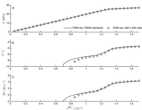
Figure 3. Evolution of (a) the mean stress, (b) the mean plastic strain, and (c) the mean plastic work during shear
banding of Test 1. The solid line corresponds to the reference FEM model (76,594 elements/230,535 nodes), and the open circles represent the results obtained with FDM (resolution of400 × 200cells). FEM = finite element method; FDM = finite difference method.
to model elastoplastic deformation and uses a Drucker-Prager model with a consistent tangent linearization. The finite element mesh is constructed with triangular elements and uses quadratic shape functions for the displacements.
We have monitored spatially averaged quantities such as the average stress (̄𝜎),
̄𝜎 = 1V∫ ∫ √𝛽JIIdV, (33)
the average plastic strain,
̄𝜖p= 1 V∫ ∫ 𝜖
p
IIdV, (34)
and average plastic work
̄ Wp= 1
V∫ ∫ W
pdV. (35)
The results obtained with FDM and with FEM are shown in Figure 3. The average stress is characterized by a period of elastic loading followed by a period of elastoplastic loading during which shear banding takes place. The transition between the two regimes occurs for a strain of approximately 1.3×10⁻³and an average stress of
approximately 2.5 MPa. The two discretization methods (FEM and FDM) result in a similar evolution and mag-nitude of the average stress, the accumulated plastic strain, and the plastic work. Differences in the average plastic strain calculated with FEM and FDM are noticeable within the first few elastoplastic strain increments. These can be explained by the different nature of the discretization methods. While the FEM allows to accu-rately resolve the inclusion/matrix boundary with an unstructured mesh, the FDM (square cells) introduces a larger discretization error. The stress field is thus better resolved in the vicinity of the inclusion with the FEM. Therefore, the onset of plastic yielding may thus not occur at the same exact loading step with the FEM and FDM (e.g.,𝜖BC≈ 0.8×10⁻³). These differences reduce as the the plastic zone develops away from the inclusion
(e.g.,𝜖BC≈ 1.2 × 10⁻³).
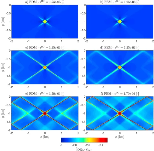
The spatial distribution of the accumulated strain for different increments is depicted in Figure 4. Shear bands start to propagate from the imperfection at a strain 1.25 × 10⁻³(Figures 4a and 4b). At a strain of 1.35 × 10⁻³,
the shear bands hit the boundaries which act as reflecting surfaces due to the free slip boundary condition (Figures 4c and 4d). At the final stage (strain level 1.75×10⁻³), the shear bands are fully developed (Figures 4e
Figure 4. Spatial distribution of the total strain during shear banding of Test 1. (a, c, e) The results obtained with FDM
and (b, d, f ) results computed with FEM. The results are shown for three different bulk strain increments (𝜖BC). FDM = finite difference method; FEM = finite element method.
and 4f ). The magnitude of the accumulated strain attained within the shear zones and the imperfection is about 5 times larger than in the least deformed parts of the domain. Overall, the results obtained with FDM and with FEM, even using various mesh resolutions, are in a good agreement (Figure 5).
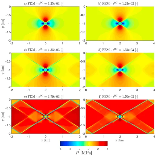
Similarly, the pressure evolution shows a good agreement (Figure 6). At the initial stages of localization (Figures 6a and 6b), the imperfection is characterized by a neutral pressure from which positive and nega-tive pressure lobes originate. As the shear band develops, the magnitude of the pressure lobes diminishes (Figures 6c and 6d) and the shear bands are characterized by a lower pressure than the adjacent, less deformed, parts of the domain (Figures 6e and 6f ).
7. Convergence of the Nonlinear Solver
A major advantage of consistent linearization is the possibility to achieve quadratic convergence of the global equilibrium equations during elastoplastic deformation. Here we report the convergence history of the force residuals during the evolution of Test 1.
All models with a grid resolution of 200 × 100 cells (Figure 5c) converged smoothly. The residuals decreased quadratically for all increments whether a line search routine was used or not. If no line search is used, the residuals initially grow before reaching a stage of quadratic convergence. The line search routine aims at min-imizing such an initial growth of residuals. For this resolution and the same applied increment, models with a (too) low value of𝛼mincan take many more nonlinear iterations to converge than models with no line search
(𝛼 = 1.0). An intermediate value of 𝛼minprovides a good compromise, leading to a moderate initial growth of
residual and a small total number of iterations (Figure 7).
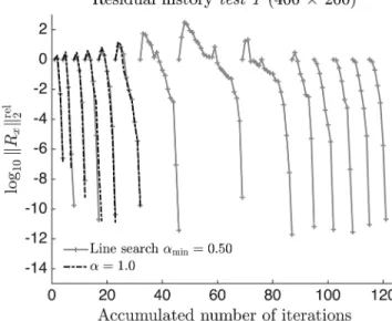
For the same increment, but a double resolution (400 × 200 cells Figure 5e), the global convergence can be slow, and divergence can occur (Figure 8), which happened when the shear bands start reflecting at the
Figure 5. Spatial distribution of the pressure (P[MPa]) during shear banding of Test 1. (a, c, e) The results obtained with FDM (resolution of200 × 100cells) and (b, d, f ) the results computed with FEM. The results are given for three different bulk strain increments (𝜖BC). FDM = finite difference method; FEM = finite element method.
domain boundaries. In these simulations, use of a line search procedure was necessary to maintain global convergence at each increment or, to be more precise, to bring the Newton-Raphson method within its radius of convergence. The underlying reason is the mechanically destabilizing influence of the nonassociated flow rule. Indeed, it has been known since the landmark paper of Rudnicki and Rice (1975) that nonassociated flow can cause loss of mechanical stability, and also loss of ellipticity, even if the material is still harden-ing. Simulations have shown that when using nonassociated plasticity, global structural softening can occur while the material is still hardening (de Borst, 1988). Moreover, it has been shown that under such condi-tions convergence deteriorates with increasing mesh refinement. It is emphasized that the fundamental, mechanical-mathematical cause of these numerical observations is the loss of ellipticity, which occurs at higher hardening rates when the difference increases between the angles of internal friction and of dilatancy.
8. Shear Banding With Von Mises and Drucker-Prager Elastoplasticity
The Von Mises and the Drucker-Prager plasticity models have been used extensively in geodynamics. Due to the pressure-insensitive character of the Von Mises model, shear bands will propagate at approximately 45∘ away from the direction of the major compressive stress. Different from this, the pressure-sensitive Drucker-Prager model yields shear bands oriented at approximately 35∘ away from the direction of the major compressive stress, depending on the precise values of the angles of friction and dilation. The results of numerical simulations using nonassociated Drucker-Prager (Test 1) and Von Mises models (Test 2) are shown in Figure 9. For the simulations with the Drucker-Prager model, shear zones initiate from the imperfection at a strain of 1.25 × 10⁻³with a characteristic angle of approximately 35∘. For the Von Mises model, shear zones
oriented at 45∘ start to propagate from the imperfection at a strain of 1.35 × 10⁻³. The shear bands
gener-ated by the Drucker-Prager model tend to be significantly more localized than those produced using the Von Mises model, but it is unclear in how far mesh sensitivity plays a role here.
Figure 6. Evolution of the relativeL2norm of residuals throughout the localization phase (i.e., from the onset of elastoplastic straining). The model configuration is Test 1 and was computed using200 × 100cells. Residual norms are reported over 14 elastoplastic strain increments. The models were run with and without line searches and using different lower bracketing limits for the line search (𝛼min). The model using𝛼min= 1.00took an accumulated number of
84 iterations, while for𝛼min= 0.05and𝛼min= 0.25, 118 and 85 iterations were respectively needed. Iterations were performed until theL2norm of residuals dropped below5.0 × 10−6, while initial values are on the order of103or104
depending on the step.
9. Shear Banding With Drucker-Prager Maxwell
Viscoelastoplasticity
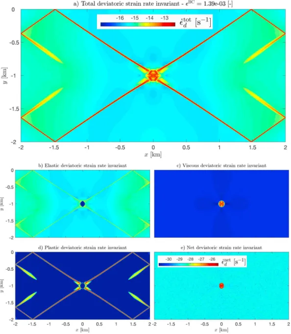
The rheological model described in the preceding section is not limited to an elastoplastic rheology and can be extended to viscous deformations. This case is particularly relevant for geodynamics applications, which generally involve frictional plastic as well as viscous strains. In model Test 3, the deformation of the elastoplastic domain is initiated by a low-viscosity circular inclusion. Such a configuration can be conceived as an analogy of a viscous magmatic body intruded in the shallow elastoplastic crust. The results of the simula-tion are given in Figure 10 for a background strain of 1.50 × 10⁻³. Strain localization leads to the formation of
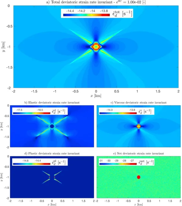
shear bands in which the effective deviatoric strain rate is 2 orders of magnitude larger than the applied strain rate (see Figure 10a). The inclusion is effectively viscous (Figure 10c), while the rest of the domain deforms partly in an elastic and partly in an elastoplastic manner (see Figures 10b and 10d). Another model (Test 4) was design to illustrate shear banding arising at a brittle-ductile transition. The viscosity of the material host-ing the inclusion is lowered by ≈ 3 orders of magnitude, and the deformation is now viscoplastic rather than elastoplastic. Shear banding initiates around the inclusion and propagates until reaching a steady state and therefore a finite length (Figure 11). It is important to notice that the additive decomposition of strain rates in viscous, elastic, and plastic contributions is exactly satisfied. This is indicated by the magnitude of the sec-ond net deviatoric strain rate invariant, which takes the form of ̇𝜖net
d = √ 1 2 ̇𝝐 net d T ̇𝝐net
Figure 7. Evolution of the relativeL2norm of residuals throughout the localization phase. The model configuration is
Test 1 and was computed using400 × 200cells. Residual norms are reported over 14 elastoplastic strain increments. The gray and black lines correspond to simulations run with and without line searches, respectively.
strain rate tensor is formulated as ̇𝝐net
d = ̇𝝐d− ( ̇𝝐e d+ ̇𝝐 v d+ ̇𝝐 p d )
. The spatial distribution of ̇𝜖net
d is depicted in
Figures 10e and 11e and its magnitude on the order of machine precision.
10. Discussion
10.1. Behavior Upon Mesh Refinement
Although the use of a consistent linearization in (visco)elastoplasticity can vastly improve the convergence speed of the iterative process that is needed to solve the nonlinear set of equations, the plasticity modeling which has been undertaken so far in crustal mechanics falls short of providing physically realistic computa-tional predictions. This is because currently used plasticity models which involve either strain weakening or nonassociated flow (or both) do not incorporate a scale dependence through the introduction of an internal length scale. Models without an internal length scale, often called local stress-strain relations, are ubiquitous in geophysics, geomechanics, and engineering and are based on the assumption that the mechanical behav-ior in a point is representative for a small but finite volume surrounding it. This assumption is often correct
Figure 8. Spatial distribution of the total strain (Test 1) after an applied background strain of1.75 × 10−3. The results
were computed with three different FDM (a, c, e) and FEM (b, d, f ) resolutions. FDM = finite difference method; FEM = finite element method.
Figure 9. Contrasting styles of shear banding with different ideal plasticity models: Drucker-Prager (Test 1) and Von
Mises (Test 2). (a, c, e) A total strain evolution for the Drucker-Prager model. (b, d, f ) The pressure-independent Von Mises model. Both models were computed using finite difference method with a grid resolution of400 × 200cells.
but fails for highly localized deformations, like fault movement or shear bands. In the presence of strain weak-ening or nonassociated flow local stress-strain relations have to be enriched to take proper account of the physical processes that occur at small length scales. A range of possibilities has been proposed to remedy this deficiency (de Borst et al., 1993), and for geodynamical applications the inclusion of a deformation-limiting viscosity, which also has been done for other crystalline solids (Needleman, 1988; Peirce et al., 1983), seems physically the most natural approach. It is emphasized, though, that not all viscoelastoplastic rheologies rem-edy this deficiency, and whether a specific rheology indeed solves the problem is dependent on the particular (parallel and/or series) arrangement of the rheological elements.
The absence of an internal length scale has a mathematical implication, as it can cause initial value prob-lems to become ill-posed (de Borst et al., 2012), which in turn causes the solutions to no longer continuously depend on the initial and boundary data. This, for instance, means that data assimilation techniques become unusable. But it also has the consequence that numerical solutions become meaningless, since they become fully dependent on the discretization (mesh dependent). This holds for any discretization method, finite ele-ments, finite differences, and also meshless methods (Pamin et al., 2003). A further consequence is that mesh refinement algorithms, which are extensively used in geodynamics (e.g., Huismans & Beaumont, 2002), will be severely biased by mesh dependence. For different initial conditions the lack of internal length scale can also result to the formation of shear bands networks with fractal distributions (Poliakov et al., 1994). For nonassociated plastic flow, convergence of nonlinear solver deteriorates when the mesh is refined (see section 7) and when the difference between the frictional and dilation angles is large. The convergence behav-ior of the supplied codes is thus not guaranteed when simulating pressure-dependent plastic flow in the incompressible limit (e.g.,𝜓 = 0, 𝜙 = 30). A detailed evaluation of the requirements needed for convergence
Figure 10. Example of shear banding using a Maxwell viscoelastoplastic rheological model (Test 3) after an applied
background strain of1.5 × 10−3. Panel (a) depicts the magnitude of the effective deviatoric strain rate (̇𝜖tot
d ). The elastic, viscous, and plastic effective deviatoric strain rates are given in panels (b), (c), and (d; similar color scale as panel a). Panel (e) depicts the magnitude of the net effective deviatoric strain rate. This model was computed with finite difference method and a grid resolution of400 × 400cells.
of simulations involving pressure-dependent plasticity in the incompressible limit is beyond the scope of this study.
10.2. Achieving High-Resolution and 3-D Modeling
In the current 2-D implementation, solutions are obtained by sparse direct factorization (i.e., Lower-Upper (LU) factorization) of the matrix operators that arise from the consistent linearization (i.e., Jacobian). In this manner, relatively high-resolution 2-D calculations can be achieved on a single-processor desktop machine. However, 3-D calculations are too time-consuming with this solution strategy. Indeed, iterative solvers are the method of choice to solve large linear systems which result from 3-D calculations. They usually require effi-cient preconditioners to unleash their full potential (Saad & van der Vorst, 2000). Preconditioners based on elastic predictor are symmetric positive definite and can thus be factored using Cholesky’s method. However,
Figure 11. Example of steady state shear banding using a Maxwell viscoelastoplastic rheological model (Test 4) after an
applied background strain of1.0 × 10−2. Panel (a) depicts the magnitude of the effective deviatoric strain rate (̇𝜖tot
d ). The elastic, viscous, and plastic effective deviatoric strain rates are given in panels (b), (c), and (d) . Panel (e) depicts the magnitude of the net effective deviatoric strain rate. This model was computed with finite difference method and a grid resolution of400 × 400cells.
they contain no information about strain localization patterns, and consequently they have very different spectral properties from the actual Jacobians, which can result in a poor performance. Pseudotransient inte-gration schemes (e.g., Gaitonde, 1994; Kelley & Keyes, 1998) or Jacobian-free Newton-Krylov techniques (e.g., Chockalingam et al., 2013; Knoll & Keyes, 2004) may be powerful alternatives for 3-D modeling of deformations in the viscoelastoplastic lithosphere.
10.3. Perspectives for Lithospheric and Geodynamic Modeling
In this study we have limited ourselves to the use of simple (single-surface) plasticity models. Future models should extend to multisurface plasticity models that can take into account the transition between tension, shear, and compaction modes. This will allow to include the effect of gravity, which leads to the occurrence of plasticity in tension for shallow crustal depths (low confining pressure), while deeper levels will rather
fol-low Drucker-Prager or Mohr-Coulomb type plasticity models. A further aspect lies in the development of multiphase flow models based on consistent linearizations in order to efficiently handle viscoelastoplastic deformations of fluid-filled porous rocks. These processes are of first-order importance for lithosphere dynam-ics since they govern the migration of magma in the lithosphere (Keller et al., 2013) or deformation patterns that can occur in sedimentary basins (Rozhko et al., 2007).
In this contribution we have followed the convention of the engineering literature to use the momentum bal-ance as point of departure, with displacements as the primitive variables. Within this context we have shown the huge potential in terms of savings in computational times and in terms of gains in accuracy that can result from the use of a consistent linearization to obtain the viscoelastoplastic tangent operator. We wish to empha-size that the application of a consistent linearization and the ensuing gains in terms of accuracy and speed are independent of the numerical method that is used to discretize the continuum. Although consistent lin-earization has almost invariably been paired to finite element discretizations in the engineering literature, this is by no means necessary, and we have used it in conjunction with the FDM which maintains a high popular-ity in the geodynamics communpopular-ity. A next step to make the technology compatible with needs and customs in this community is to switch to a flow formulation, with velocities and pressures as the primitive variables. This requires some subtle modifications to the linearization but is generally fairly straightforward.
11. Conclusions
We have introduced the use of the consistent tangent operator in (visco)elastoplasticity to solve deformation problems that are classically encountered in lithosphere dynamics within the framework of a finite differ-ence formulation. This approach allows the efficient solution of plastic strain localization problems at the kilometer scale. Quadratic convergence was obtained for models which involved the pressure-insensitive Von Mises model and the pressure-dependent Drucker-Prager yield contour. The implementation was verified quantitatively and qualitatively with results obtained using an independent finite element package. A minor modification in the algorithm enables to also take into account viscous creep. Such a consistent tangent operator for viscoelastoplasticity is essential for geodynamic modeling which needs to accurately capture pressure-dependent frictional plastic deformation as well as viscous creep at the kilometer scale. Finally, concise and fast model implementations have been made available as a subset of M2Di MATLAB routines (https://bitbucket.org/lraess/m2di) and all results are fully reproducible.
Appendix A: The Viscoelastic Tangent Operator
The additive decomposition of the deviatoric strain rate ̇𝝐′can be written as
̇𝝐′=(̇𝝐e)′
+(̇𝝐v)′= ̇𝝉
2G+ 𝝉2𝜂. (A1)
Using a backward Euler rule, so that ̇𝝐′= Δ𝝐′
Δt, one obtains Δ𝝐′= ( 1 2G+ Δt 2𝜂 ) 𝝉t+1− 𝝉t 2G. (A2)
With the identity𝝉t+1=𝝉t+ Δ𝝉 and Gve= ( 1 G+ Δt 𝜂 )−1 , 𝜉 = Gve G ,
the incremental update rule for the deviatoric stress is written as
Δ𝝉 = 2GveΔ𝝐′+ (𝜉 − 1) 𝝉t. (A3)
The total stress update reads
𝝈t+1= −Pti +𝝉t− ΔPi + Δ𝝉 (A4)
with, for plane-strain conditions, iT = [1, 1, 1, 0]. Substitution of the expressions for Δ𝝉 and ΔP then leads to
Figure A1. Verification of the implementation of the viscoelastic rheological model. (a) The evolution of the deviatoric
stress (𝜏xx) and pressure (P) in a homogeneous domain subjected to pure shear kinematics. The deviatoric rheology is viscoelastic. (b) The evolution of the deviatoric stress and pressure inside a layer oriented parallel to the compression direction (pure shear kinematics). The deviatoric rheology is purely viscous (the layer is 1 order of magnitude more viscous than the matrix), but the bulk rheology is elastically compressible.
with the viscoelastic tangent operator Dvedefined as
Dve= ⎡ ⎢ ⎢ ⎢ ⎢ ⎣ K +4 3G ve K −2 3G ve K −2 3G ve 0 K −2 3G ve K +4 3G ve K −2 3G ve 0 K −23Gve K −2 3G ve K +4 3G ve 0 0 0 0 Gve ⎤ ⎥ ⎥ ⎥ ⎥ ⎦ . (A6)
The verification of this algorithm for the stress evolution has been carried out in two steps. The first test has been carried out for a viscoelastic shear rheology, considering a homogeneous domain undergoing pure shear. For this case, an analytical solution exists and takes the form
𝜏analytical xx =𝜎xxff [ 1 − exp(− t tMaxwell )] , (A7) where𝜎ff
xx= 2𝜂 ̇𝜖xxis the far-field stress (assuming far-field pressure is equal to 0) and tMaxwell= 𝜂G. Figure A1a
shows that the computed deviatoric stress closely follows the analytical solution for the buildup of the vis-coelastic stress. This case only involves deviatoric strains, and therefore the pressure buildup is negligible. A convergence test reveals the expected first-order convergence of the numerical solution toward the analytical solution. For the reference Δt = 104the L
1error norm is 1.11 × 10⁻². This error diminishes down to 5.6 × 10⁻³
and 2.8 × 10⁻³for values of divided Δt divided by a factor 2 and 4, respectively.
For this reason a case was considered in which a layer oriented parallel to the compressive direction and 0.3 times the height of the domain is taken into account (Moulas et al., 2018). Here the rheology is purely viscous for the stress deviators (by letting G → ∞) and is purely elastic for the pressure. The layer is 10 times more viscous than the embedding matrix. The results shown in Figure A1b are in agreement with those of Moulas et al. (2018). The pressure difference between the layer and the matrix (ΔP) evolves as
ΔPanalytical= Δ𝜎xxff [ 1 − exp(−3 4 t tMaxwell )] , (A8)
and the difference in deviatoric stress between the layer and matrix the matrix follows Δ𝜏xxanalytical= −Δ𝜎xxff [1 −1 2exp ( −3 4 t tMaxwell )] . (A9)
In this case, the Maxwell time is defined as tMaxwell= 𝜂layer
Klayerand Δ𝜎 ff xx= −Player+ 2 ( 𝜂layer−𝜂matrix ) ̇𝜖xxstands for
the layer/matrix total stress difference in the far field (assuming far-field pressure in the layer is equal to 0) .
Appendix B: The Viscoelastic-Plastic Consistent Tangent Operator
For viscoelastoplastic straining, the stress update reads𝝈t+1= −Pti +𝜉𝝉t+ DveΔ𝝐 − Δ𝜆Dve𝜕Q
𝜕𝝈. (B1)
A small variation𝛿 of the updated stress 𝝈t+1is then given by 𝛿𝝈 = Dve𝛿𝝐 − 𝛿𝜆Dve𝜕Q
𝜕𝝈 − Δ𝜆Dve𝜕
2Q
𝜕𝝈2𝛿𝝈 , (B2)
which can be rewritten as
𝛿𝝈 = E−1Dve𝛿𝝐 − E−1Dve𝜕Q
𝜕𝝈𝛿𝜆 (B3)
with
E = I + Δ𝜆D 𝜕2Q
𝜕𝝈2. (B4)
Similarly, a variation of the yield condition
F(𝝈t+1) = 0 (B5) leads to ( 𝜕F 𝜕𝝈 )T 𝛿𝝈 = 0 , (B6)
which can interpreted as the consistency condition, which must be satisfied during plastic loading. Premul-tiplying equation (B3) by(𝜕𝝈𝜕F)
T
and invoking condition (B6) yields an explicit expression for the variation of the plastic multiplier:
𝛿𝜆 = (𝜕F 𝜕𝝈 )T E−1Dve (𝜕F 𝜕𝝈 )T E−1Dve 𝜕Q 𝜕𝝈 𝛿𝝐 . (B7)
The final step in the construction of the consistent tangent operator is the substitution of the variation of the plastic multiplier into equation (B3), leading to
𝛿𝝈 = ⎛ ⎜ ⎜ ⎜ ⎝ E−1Dve− E−1Dve 𝜕Q 𝜕𝝈 (𝜕F 𝜕𝝈 )T E−1Dve (𝜕F 𝜕𝝈 )T E−1Dve 𝜕Q 𝜕𝝈 ⎞ ⎟ ⎟ ⎟ ⎠ 𝛿𝝐 . (B8) Since by definition Dvep≡ 𝜕𝝈 𝜕𝝐, (B9)
Figure C1. Verification of the implementation of the viscoelastoplastic rheological model (Test 4). (a) The evolution of
the effective stress (̄𝜎). (b) The evolution of the error in effective stress relative to the high time resolution run (̄𝜎err). (c) The magnitude of the maximum stress error as a function of the time step magnitude.
the viscoelastoplastic consistent tangent operator Dvep takes the form
Dvep= E−1Dve− E−1Dve 𝜕Q 𝜕𝝈 ( 𝜕F 𝜕𝝈 )T E−1Dve ( 𝜕F 𝜕𝝈 )T E−1Dve 𝜕Q 𝜕𝝈 . (B10)
All the elements of the consistent tangent operator, that is, Δ𝜆,𝜕𝝈𝜕F,𝜕Q𝜕𝝈,𝜕𝜕𝝈2Q2, can be obtained analytically from
the current stress state, either at integration points or at finite difference cell centers and vertices. The inverse of E is obtained analytically by local matrix inversion, which avoids potential inaccuracies due to numerical approximations of the inverse of E (de Borst & Groen, 1994).
Appendix C: Convergence in Time of Discrete Viscoelastic-Plastic Rheology
A backward Euler rule was employed to discretize the entire rheological model at the local level (cell cen-ters/vertices for FDM or integration points for FEM). The drawback of this approach is that an explicit dependence on the time step (Δt) is introduced into the rheological coefficients (see, e.g., equation (A2)). With the displacement-based formulation the standard elastic rheological model is recovered by letting𝜂 → ∞ or Δt→ 0. This contrasts with velocity-based formulations (Gerya & Yuen, 2007; Moresi et al., 2002; Schmalholz et al., 2001) for which backward Euler time discretization introduces Δt in the denominator of the effective rheological coefficient and is thus invalid in the limit Δt→ 0. Such formulation is likely beneficial as it is com-mon practice to decrease Δt to reduce time integration error, to resolve physical processes occurring on short time scales (e.g., seismic cycle modeling), or to allow for solving nonlinear problems (i.e., time step adaptivity). Here we verify that our formulation converges with increasing time resolution using Test 4 for which all ele-ments of the rheological chain are solicited (cf. Figure 11). There exists no analytical solution for predicting the transient evolution of the model; therefore, we use results computed at a high time resolution as reference. Models were computed with larger time steps [0.5Δt, Δt, 2Δt, 4Δt, 8Δt], and the error in stress were com-puted relative to the smallest time step (0.5Δt). The evolution of effective stress ( ̄𝜎 = 1V∫∫ √𝛽JIIdV) for the
different values of Δt is depicted in Figure C1a. The error in effective stress,̄𝜎err, is reported in in Figure C1b,
which clearly shows a decrease of the error with a decrease of Δt. A closer look (Figure C1c) reveals that the maximum error decrease by a factor ≈ 2 for a reduction of Δt by a factor 2, which indicates a first-order convergence as expected for backward Euler time integration.
References
Buiter, S. J. H., Babeyko, A. Y., Ellis, S., Gerya, T. V., Kaus, B. J. P., Kellner, A., et al. (2006). The numerical sandbox: Comparison of model results for a shortening and an extension experiment. Geological Society, London, Special Publications, 253(1), 29–64. https://doi.org/10.1144/GSL.SP.2006.253.01.02
Buiter, S. J., Schreurs, G., Albertz, M., Gerya, T. V., Kaus, B., Landry, W., et al. (2016). Benchmarking numerical models of brittle thrust wedges.
Journal of Structural Geology, 92, 140–177. https://doi.org/10.1016/j.jsg.2016.03.003
Chockalingam, K., Tonks, M. R., Hales, J. D., Gaston, D. R., Millett, P. C., & Zhang, L. (2013). Crystal plasticity with Jacobian-free Newton-Krylov.
Computational Mechanics, 51(5), 617–627.
Choi, E., Lavier, L., & Gurnis, M. (2008). Thermomechanics of mid-ocean ridge segmentation. Physics of the Earth and Planetary Interiors,
171(1), 374–386. recent Advances in Computational Geodynamics: Theory, Numerics and Applications.
Choi, E., & Petersen, K. D. (2015). Making Coulomb angle-oriented shear bands in numerical tectonic models. Tectonophysics, 657, 94–101. https://doi.org/10.1016/j.tecto.2015.06.026
Cundall, P. A. (1989). Numerical experiments on localization in frictional materials. Ingenieur-Archiv, 59, 148–159.
Dabrowski, M., Krotkiewski, M., & Schmid, D. W. (2008). Milamin: Matlab-based finite element method solver for large problems.
Geochem-istry, Geophysics, Geosystems, 9, Q04030. https://doi.org/10.1029/2007GC001719
de Borst, R. (1988). Bifurcations in finite element models with a non-associated flow law. International Journal for Numerical and Analytical
Methods in Geomechanics, 12, 99–116.
de Borst, R. (1989). Numerical methods for bifurcation analysis in geomechanics. Ingenieur-Archiv, 59, 160–174.
de Borst, R., Crisfield, M. A., Remmers, J. J. C., & Verhoosel, C. V. (2012). Non-linear finite element analysis of solids and structures (2nd ed.). Chichester: Wiley.
de Borst, R., & Feenstra, P. H. (1990). Studies in anisotropic plasticity with reference to the Hill criterion. International Journal for Numerical
Methods in Engineering, 29, 315–336.
de Borst, R., & Groen, A. E. (1994). A note on the calculation of consistent tangent operators for von Mises and Drucker-Prager plasticity.
Communications in Numerical Methods in Engineering, 10, 1021–1025.
de Borst, R., Sluys, L. J., Mühlhaus, H.-B., & Pamin, J. (1993). Fundamental issues in finite element analysis of localisation of deformation.
Engineering Computations, 10, 99–122.
Evans, B., Fredrich, J. T., & Wong, T.-F. (1990). “The brittle-ductile transition in rocks: Recent experimental and theoretical progress” (Vol. 56, pp. 1–21). New York: American Geophysical Union.
Fossen, H. (2016). Structural geology (2nd ed.). Cambridge: Cambridge University Press.
Fullsack, P. (1995). An arbitrary Lagrangian-Eulerian formulation for creeping flows and its application in tectonic models. Geophysical
Journal International, 120(1), 1–23.
Gaitonde, A. L. (1994). A dual-time method for the solution of the unsteady Euler equations. The Aeronautical Journal (1968), 98(978), 28391. https://doi.org/10.1017/S0001924000026786
Gerbault, M., Hassani, R., Novoa, L. C., & Souche, A. (2018). Three-dimensional failure patterns around an inflating magmatic chamber.
Geochemistry, Geophysics, Geosystems, 19, 749–771. https://doi.org/10.1002/2017GC007174
Gerya, T. V., & Yuen, D. A. (2003). Characteristics-based marker-in-cell method with conservative finite-differences schemes for modeling geological flows with strongly variable transport properties. Physics of the Earth and Planetary Interiors, 140(4), 293–318.
Gerya, T. V., & Yuen, D. A. (2007). Robust characteristics method for modelling multiphase visco-elasto-plastic thermo-mechanical problems.
Physics of the Earth and Planetary Interiors, 163(1), 83–105.
Huismans, R. S., & Beaumont, C. (2002). Asymmetric lithospheric extension: The role of frictional plastic strain softening inferred from numerical experiments. Geology, 30(3), 211.
Kaus, B. J. P. (2010). Factors that control the angle of shear bands in geodynamic numerical models of brittle deformation. Tectonophysics,
484, 36–47. https://doi.org/10.1016/j.tecto.2009.08.042
Keller, T., May, D. A., & Kaus, B. J. P. (2013). Numerical modelling of magma dynamics coupled to tectonic deformation of lithosphere and crust. Geophysical Journal International, 195(3), 1406–1442. https://doi.org/10.1093/gji/ggt306
Kelley, C., & Keyes, D. (1998). Convergence analysis of pseudo-transient continuation. SIAM Journal on Numerical Analysis, 35(2), 508–523. https://doi.org/10.1137/S0036142996304796
Knoll, D., & Keyes, D. (2004). Jacobian-free Newton-Krylov methods: A survey of approaches and applications. Journal of Computational
Physics, 193(2), 357–397.
Le Pourhiet, L. (2013). Strain localization due to structural softening during pressure sensitive rate independent yielding. Bulletin de la
Société Géologique de France, 184(4-5), 357.
Lemiale, V., Mühlhaus, H.-B., Moresi, L., & Stafford, J. (2008). Shear banding analysis of plastic models formulated for incompressible viscous flows. Physics of the Earth and Planetary Interiors, 171, 177–186.
Moresi, L., Dufour, F., & Mühlhaus, H.-B. (2002). Mantle convection modeling with viscoelastic/brittle lithosphere: Numerical methodology and plate tectonic modeling. Pure and Applied Geophysics, 159(10), 2335–2356.
Moresi, L., Mühlhaus, H.-B., Lemiale, V., & May, D. (2007). Incompressible viscous formulations for deformation and yielding of the litho-sphere. Geological Society, London, Special Publications, 282(1), 457–472. https://doi.org/10.1144/SP282.19
Moulas, E., Schmalholz, S. M., Podladchikov, Y., Tajcmanová, L., Kostopoulos, D., & Baumgartner, L. (2018). Relation between mean stress, thermodynamic and lithostatic pressure. Journal of Metamorphic Geology. https://doi.org/10.1111/jmg.12446
Needleman, A. (1988). Material rate dependence and mesh sensitivity in localization problems. Computer Methods in Applied Mechanics and
Engineering, 67, 69–85.
Olive, J.-A., Behn, M. D., Mittelstaedt, E., Ito, G., & Klein, B. Z. (2016). The role of elasticity in simulating long-term tectonic extension.
Geophysical Journal International, 205(2), 728–743.
Pamin, J., Askes, H., & de Borst, R. (2003). Two gradient plasticity theories discretized with the element-free Galerkin method. Computer
Methods in Applied Mechanics and Engineering, 192, 2377–2403.
Passchier, C. W., & Trouw, R. A. J. (1996). Microtectonics. Berlin: Springer.
Peirce, D., Asaro, R. J., & Needleman, A. (1983). Material rate dependence and localized deformation in crystalline solids. Acta Metallurgica,
31, 1951–1076.
Poliakov, A., & Podladchikov, Y. Y. (1992). Diapirism and topography. Geophysical Journal International, 109(3), 553–564. Poliakov, A. N. B., Herrmann, H. J., Podladchikov, Y. Y., & Roux, S. (1994). Fractal plastic shear bands. Fractals, 02(04), 567–581.
https://doi.org/10.1142/S0218348X9400079X
Popov, A. A., & Sobolev, S. V. (2008). SLIM3D: A tool for three-dimensional thermomechanical modeling of the lithospheric deformation with elasto-visco-plastic rheology. Physics of the Earth and Planetary Interiors, 171, 55–75.
Acknowledgments
The authors acknowledge two anonymous reviewers as well as the Associate Editor for providing insightful reviews. The authors wish to thank Vangelis Moulas and Yury Podladchikov for the numerous intense discussions. The authors wish to thank the NETHERMOD 2017 and GEOMOD 2016 conference organizers. Financial support from the European Research Council (ERC Advanced grant 664734) and from the Research Council of Norway (DIPS project, grant 240467) are gratefully acknowledged. MATLAB scripts and Jupyter notebooks are available at https://bitbucket.org/ lraess/m2di.

![Figure 5. Spatial distribution of the pressure ( P [MPa]) during shear banding of Test 1](https://thumb-eu.123doks.com/thumbv2/123doknet/14797711.604689/11.918.305.816.134.637/figure-spatial-distribution-pressure-mpa-shear-banding-test.webp)