HAL Id: hal-00185999
https://hal.archives-ouvertes.fr/hal-00185999
Submitted on 31 Oct 2018
HAL is a multi-disciplinary open access
archive for the deposit and dissemination of
sci-entific research documents, whether they are
pub-lished or not. The documents may come from
teaching and research institutions in France or
abroad, or from public or private research centers.
L’archive ouverte pluridisciplinaire HAL, est
destinée au dépôt et à la diffusion de documents
scientifiques de niveau recherche, publiés ou non,
émanant des établissements d’enseignement et de
recherche français ou étrangers, des laboratoires
publics ou privés.
Revolving rivers in sandpiles: from continuous to
intermittent flows
E. Altshuler, R. Toussaint, E. Martinez, O. Sotolongo-Costa, J. Schmittbuhl,
K. J. Måløy
To cite this version:
E. Altshuler, R. Toussaint, E. Martinez, O. Sotolongo-Costa, J. Schmittbuhl, et al.. Revolving rivers in
sandpiles: from continuous to intermittent flows. Physical Review E : Statistical, Nonlinear, and Soft
Matter Physics, American Physical Society, 2008, 77 (3), pp.031305. �10.1103/PhysRevE.77.031305�.
�hal-00185999�
Revolving rivers in sandpiles: From continuous to intermittent flows
E. Altshuler,1,2R. Toussaint,2 E. Martínez,1O. Sotolongo-Costa,1 J. Schmittbuhl,2and K. J. Måløy31“Henri Poincaré” Group of Complex Systems, Physics Faculty, University of Havana, 10400 Havana, Cuba 2
Institute of Globe Physics in Strasbourg, UMR 7516 CNRS, Université Louis Pasteur, 5 rue Descartes, F-67084 Strasbourg Cedex, France
3
Department of Physics, University of Oslo, P.O. Box 1048 Blindern, 0316 Oslo, Norway 共Received 6 November 2007; published 17 March 2008兲
In a previous paper关E. Altshuler et al., Phys. Rev. Lett. 91, 014501 共2003兲兴, the mechanism of “revolving rivers” for sandpile formation is reported: As a steady stream of dry sand is poured onto a horizontal surface, a pile forms which has a river of sand on one side flowing from the apex of the pile to the edge of the base. For small piles the river is steady, or continuous. For larger piles, it becomes intermittent. In this paper we establish experimentally the “dynamical phase diagram” of the continuous and intermittent regimes, and give further details of the piles’ “topography,” improving the previous kinematic model to describe it and shedding further light on the mechanisms of river formation. Based on experiments in Hele-Shaw cells, we also propose that a simple dimensionality reduction argument can explain the transition between the continuous and inter-mittent dynamics.
DOI:10.1103/PhysRevE.77.031305 PACS number共s兲: 45.70.Mg, 45.70.Qj, 83.80.Fg
I. INTRODUCTION
When most granular materials are poured onto a horizon-tal surface, a conical pile builds up through an avalanche mechanism involving all the surface of the pile that “tunes” the angle of repose about a certain critical value. In a previ-ous paper, however, we reported a different mechanism of sandpile formation 关1兴. In those experiments, as the pile
grows, a river of sand spontaneously builds up, flowing down one side of the pile from the apex to the base. The river then begins to revolve around the pile, depositing an helical layer of material with each revolution, causing the pile to grow. Below a certain pile size and input flux, the rivers are continuous, and the surface of the pile is smooth共see upper inset in Fig.1兲. The revolving direction can be either
clock-wise or counterclockclock-wise, only depending on random fluc-tuations in the first stage of the experiment. For bigger piles, the rivers are intermittent, and the surface of the pile become undulated共see lower inset in Fig.1兲. Kong and co-workers
关2兴 reported a detailed computational model for the revolving
rivers which manages to reproduce many of their features in the continuous regime, but the intermittent regime was not accounted for. They also noticed that the details of the grain-grain interactions must be tuned in order to get the revolving rivers, which matches the experimental fact that not all sands display such behavior. In this paper, we explore experimen-tally the “dynamic phase diagram” of the different regimes in our sandpiles 共i.e., the regions of experimental parameters where they appear兲. We report the details of the “topogra-phy” of the sandpiles in the continuous and intermittent re-gimes, and present a refined “kinetic” description of the ob-served phenomena. We then propose an explanation for the existence of two types of revolving rivers based on an anal-ogy with measurements performed in a simpler geometry 共i.e., the Hele-Shaw cell兲.
II. “DYNAMIC PHASE DIAGRAM” OF THE REVOLVING RIVERS
We used sand with a high content of silicon oxide from Santa Teresa共Pinar del Río, Cuba兲 关1,3兴. The grain size
dis-tribution is basically a Gaussian disdis-tribution centered at 200 m, with a half-width slightly smaller than 200 m. From now on, we will adopt the labeling of Ref.关1兴 for the
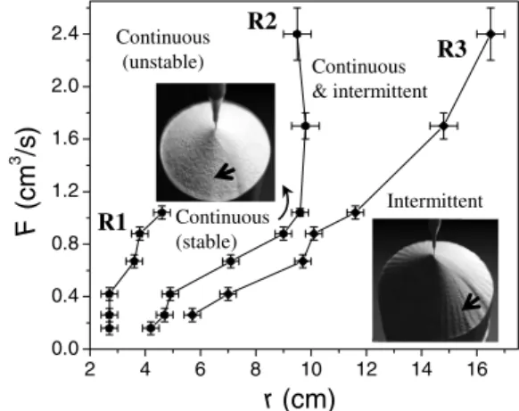
boundary conditions used in each experiment: BCI stands for a pile grown on a closed cylindrical container with a flat, horizontal bottom, and BCII corresponds to a pile formed on an open, flat horizontal surface. To obtain the dynamic phase diagram, we grew piles in boundary condition BCII. We used glass funnels of various diameters to obtain different values of the input flux. It was determined in each experiment by measuring the volume of the conical pile, and dividing it by the time elapsed since the first grains were dropped on the table. For a given input flux, three different pile base radii were identified by simple observation as the pile grew. Be-low r1, continuous rivers appeared and disappeared共as even-tually happens in common sands兲, so we will refer to them as unstable. Above r1 and below r2, a stable continuous river revolved around the pile in a given direction, without any
Continuous (unstable) Continuous (stable) Continuous & intermittent Intermittent R1 R2 R3 2 4 6 8 10 12 14 16 0.0 0.4 0.8 1.2 1.6 2.0 2.4 F (cm 3 /s) r (cm)
FIG. 1. Occurrence of continuous and intermittent rivers as functions of the pile radius r and the input flux F. The upper and lower insets show snapshots of the pile during the共stable兲 continu-ous and the intermittent regimes, respectively. The arrows indicate the direction of revolution around the pile.
major changes in its shape. After r2, the continuous river could eventually become intermittent: The downhill flow would suddenly stop at the edge of the pile, and a “finger” of sand would escalate from bottom to top, like a “stop-up” front 关4兴. All in all, the continuous or intermittent rivers
would keep revolving around the pile with the frequency described in 关1兴 共see also Fig.7兲. However, at some point
this process transformed again into a continuous, revolving river. As the radius of the pile grew from r2 to r3, the inter-mittent mechanism took place within larger and larger time intervals, while the continuous mechanism slowly disap-peared. At r3, intermittent rivers were established as the only dynamical phase in the pile. As r1, r2, and r3 were deter-mined for various input fluxes, three boundaries R1, R2, and R3 were established to separate the different dynamical phases, as shown in Fig.1. We have observed that the posi-tions of these lines are influenced by the distance between the funnel that delivers the sand and the tip of the pile, but we kept this distance fixed at approximately 2 cm during the experiments. It should be noticed that, for input fluxes larger than approximately 1 cm3/s, stable continuum rivers are
never established, and a direct transition from unstable con-tinuous to intermittent rivers takes place through R2.
III. REFINED KINEMATIC MODEL
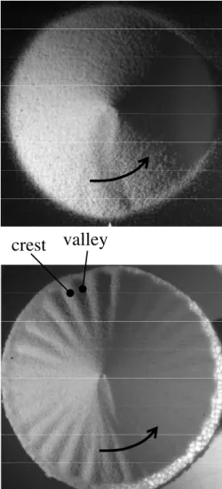
Figure2shows images taken from top of “frozen” piles in the stable continuous 共upper panel兲 and intermittent 共lower panel兲 regimes obtained for boundary condition BCII. Piles were formed using a steady input flux, which was just switched off to take the pictures. In both images, the river can be identified as a curved groove from the apex to the base of the pile, in a general vertical direction, below the apex. In order to quantify the topography of the piles共at least for one size兲, we measured its slope angle 共polar angle兲 ver-sus the angle around the pile 共azimuthal angle兲. The mea-surement was performed by carefully setting a ruler tangen-tial to the slope of the pile at different azimuthal angles, taking a lateral picture of the system, and calculating the angles between the ruler and the horizontal from the result-ing images. This ruler was set along the section of the slope where the angle is essentially constant 共this angle becomes smaller at a few cm from the top of the piles兲. Figure 3
shows how the slope angle depends on the azimuthal angle for the case of the continuous rivers. Contrary to the first impression when the picture of the upper panel of Fig.2 is examined, there is a wide angular zone of variation of the slope angle, quantified in Fig. 3. This suggests that, while most of the downhill flow is concentrated into the relatively narrow river clearly visible below the apex of the pile共upper panel of Fig.2兲, there is a wider area of grains rolling
down-hill. The slope angle is typically around 36.5° far from the river. It significantly decreases to 33° within the river. The width of the low slope angle region extends over 150° along the azimuthal direction. This corresponds to a length of around 28 cm along the circumference of the pile, which is much larger than the river 共which is a few cm wide兲. To illustrate this, Fig.4 shows the difference between two im-ages of a sandpile grown in BCI in the continuous regime,
separated by a lapse of 0.15 s 共the video was taken by a Photon Fastcam Ultima-ADX model 120K, and the image was obtained using the “difference” option of ImageJ兲. Be-sides the fast flow along the main stream of the river, whiter and darker spots indicate the downhill movement of sand at a smaller speed behind the main stream area.
The situation is quite different in the case of the intermit-tent regime. The measurement of the angles of repose of several “valleys” and “crests” corresponding to the picture in the lower panel of Fig.2does not indicate a wide transition in the angle of repose, as in the case of the continuous rivers, but suggests two basic polar angles: 37.1°⫾0.16°, for the valleys, and 36.1°⫾0.20° for the crests. It should be no-ticed, however, that the pile in the intermittent regime con-tains an inner circle where the surface is smooth, and an outer ring of undulating surface, as seen in Fig. 2 共lower
panel兲. The values we have reported here for the slope angles at the valleys and crests correspond to this ring of
approxi-crest valley
FIG. 2. Topography of the continuous and intermittent regimes. Upper panel: Top view showing a pile “frozen” during a continuous river experiment. The diameter of the pile is 11 cm. Lower panel: Top view of a pile “frozen” during an intermittent river experiment. The diameter of the pile is 17 cm—surface undulations extend ap-proximately 6 cm from the edge of the pile in the radial direction. Black arrows on top of the flowing river indicate the direction of revolution of the rivers as sand is added from above.
ALTSHULER et al. PHYSICAL REVIEW E 77, 031305共2008兲
mately 6 cm width in the radial direction, while the average slope of the pile in the inner circle is harder to measure due to rounding near the apex of the pile.
The phenomenological model for the revolving rivers pre-sented in Ref.关1兴 is able to predict the radius and time
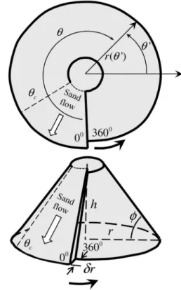
de-pendence of the frequency of revolution of the piles, but oversimplifies the geometry of the sandpile in such a way that the angle of repose is constant around the pile, in con-tradiction with the real topography shown in Fig.2and quan-tified in Fig. 3. We present here a more realistic model, which is schematized in Fig.5 for BCII. This model has a number of advantages relative to the one presented in Ref. 关1兴. First, it takes into account that the apex of the pile is not
sharp, but presents a small “crater”共very exaggerated in the schematics shown in Fig.5兲. Second, the river, located in the
section on the cone on which the sand flows, has a nonzero width. Third, the angle of repose is not constant around the pile, but can be shaped as depicted in Fig.5, where the width of the downhill flowing area has been tuned to 150° in the azimuthal direction共the figure displays a smaller angle兲. We add two further constraints, which roughly match
experimen-tal observations: The characteristic length␦r is constant, and so is the radius of the crater.
The geometry of the pile, in the continuous regime, can be schematized as follows:
We define an azimuthal coordinate around the pile in a frame co-moving with the revolving river, so that= 0 cor-responds to the position of the flowing river, where most of the flow is located. In the reference frame of the laboratory, the azimuthal coordinate
⬘
is ⬘
=0共t兲−, where 0共t兲 =0共0兲+兰0t
共t
⬘
兲dt⬘
is the azimuthal angle of the river, and共t兲=˙
0共t兲 is the instantaneous angular velocity of the
re-volving river.
The radius of the bottom of the pile is fixed after the river has added a layer of thickness ␦r: This radius is denoted r共
⬘
兲. There is no evolution of this radius apart from the outlet of the concentrated river, i.e., any other surface flow than the river on the sides of the pile does not reach the bottom. This radius jumps by a characteristic length ␦r = r共⬘
+ 360°兲−r共⬘
兲 at each passing of the river, which adds a new layer of grains to the pile. This jump corresponds to the distance over which grains flowing down the pile at a characteristic speed, dissipate entirely their kinetic energy over the flat bottom. This jump has a characteristic value around 4 mm.Calling h共t兲 the height of the center of the pile, there is a small crater forming around this tip. The crater corresponds θ
φ
0 50 100 150 200 250 300 350 32 33 34 35 36 37 38 A ngl e o f re pose, (degrees)Angle around the pile, (degrees)
FIG. 3. Dependence of the angle of repose on the azimuthal angle for the picture of the upper panel of Fig.2共continuous river兲.
The “0” of the azimuthal angle has been taken along the vertical diameter under the apex, and it increases clockwise. The error bars correspond to the largest variation of the measured angles of repose in three different attempts on the same pile.
FIG. 4. Moving grains in the continuous river regime. The figure is the difference between two pictures of a continuous river sepa-rated by 0.15 s共the river was revolving around the pile at approxi-mately 0.1 turns/s兲. This difference is superimposed with the first of these two pictures. The arrow indicates the direction of the revolu-tion of the river around the pile. The inset shows a raw picture of the crater, at the upper end of the pile.
FIG. 5. Diagram of the model used to estimate the revolving speed of the rivers, and the polar bottom angle versus the azimuthal angle. Upper panel: Top view of the pile model. Lower panel: Spa-tial view of the pile model共notice that the angle of the flowing zone has been decreased in this representation relative to the top view, to improve drawing clarity兲. The black arrows indicate the direction of revolution around the pile.
then to a sharp crest around the center of the pile, slightly higher than the central point, and exists for azimuthal angles
betweencand 360°. A characteristic value observed forc
is around 150°, as pointed out before. There is no observed surface flow on the sides of the pile below this crater crest, i.e., the surface of the pile corresponding toc⬍⬍360° is
frozen. The crater crest lies at a height␦h共兲 above the cen-ter, i.e., at an altitude h共t兲+␦h共兲: The crater shape revolves at the same speed as the flowing river. In the reference frame of the bottom plate, a point of the crest is also fixed, i.e., h共t兲+␦h关0共t兲−
⬘
兴 is constant, so its time derivative is h˙+共d␦h/d兲= 0: The crater has a screwlike shape, with an azimuthal slope of the crest共d␦h/d兲=−h˙/set by the ratio between the pile rising speed and the revolving angular ve-locity.
After the passing of the river, there is a small surface flux, visible as a few whiter and darker dots on Fig.4, increasing the effective angle of the slope, as seen in Fig.3. This sur-face flow happens for azimuthal angles between 0° 共the river兲 andc. The tip of the pile, for these angles, presents no
change of sign of the radial slope 共no crater crest兲. For larger thanc, the crest of the crater at the tip of the pile is
formed around the central point, i.e., noting S共r,兲 the coor-dinates of the surface of the pile, the radial slope ofS/r is positive for low radii r, and negative for larger ones, after the crest. At these angles, this crest prevents further surface flow on the sides of the pile, so that the rest共polar兲 angle ⌽0共兲 is
frozen at a roughly constant value betweenc共the beginning
of the crest兲 and = 360°. To illustrate this organization, a collection of schematic cuts of the pile side at various azi-muth is shown in Fig.6.
The role of this crater on the organization of the flow in revolving rivers seems thus very important. For example,
when the incoming sand flux presents too many lateral oscil-lations or is too wide, the crater and revolving river forma-tion are prevented. Similarly, when the pile has not grown enough to reach a diameter beyond the distance of saltation from the impact point, the crater formation is prevented, and unstable rivers are observed, i.e., beyond the line R1 in Fig.
1. The fact that grains do not bounce too far when they arrive on the pile, i.e., a moderate restitution coefficient, is certainly an important ingredient to allow for the crater formation.
From this geometry, one can also infer a relationship be-tween the pile radius and the angular velocity, as reported in 关1兴: During a time dt, a volume of sand Fdt is deposited over
a layer of size ␦r tan共⌽0兲r2dt/2, where ⌽
0 is the repose
angle along most of the pile共for azimuth betweencand
360°兲. Consequently, mass conservation of the grains im-poses that = 2F/关r2␦r tan共⌽
0兲兴. This power-law
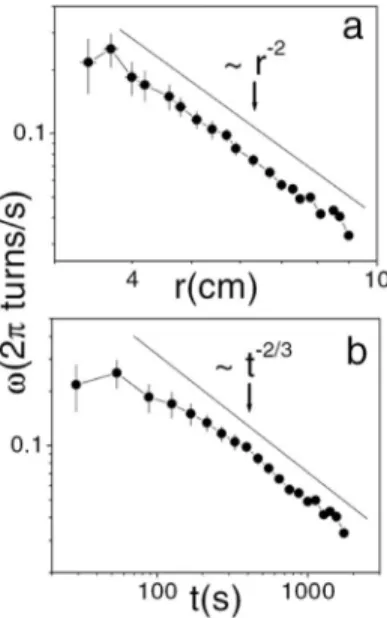
depen-dence of the angular velocity over the pile radius is verified experimentally, as shown in Fig. 7. Since the pile radius increases from flux conservation so that r共t兲3tan共⌽0兲/3
= Ft, i.e., as r共t兲=关3Ft/tan共⌽0兲兴1/3, the angular velocity
goes as =共/3兲2/3 2F 1/3 ␦r共tan ⌽0兲1/3 1 t2/3. 共1兲
This power law decrease of the angular velocity with time is also verified experimentally共Fig.7兲.
At a certain critical size of the pile radius rci, the flow
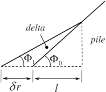
becomes intermittent and exhibits avalanches, while still be-ing concentrated along a river. These avalanches extend over a basis␦r from the pile bottom, comparable to the horizontal extent of layers added by the flowing river in the continuous regime. These avalanches form delta-shaped piles on the side of the main cone, with a slightly carved river penetrating above the apex of the delta共as seen below the pile’s apex, lower panel of Fig.2兲 which is “smoothed out” as the river
r
( , ) S r θ ( , ) S rθ ( ) h t ( ) dhθ ( ) h t ( ) dhθ c θ θ= c θ θ= 360o θ = 0o θ=r
FIG. 6. Cuts of the pile side at constant azimuth in the con-tinuous regime. Upper panel: Frozen side of the pile, below a crater crest. Lower panel: Part where the revolving river passes, and where the surface flow takes place behind it.
FIG. 7. Radius共a兲 and time 共b兲 dependencies of the frequency of revolution of the rivers共taken from 关1兴兲. The points correspond
to experimental values.
ALTSHULER et al. PHYSICAL REVIEW E 77, 031305共2008兲
moves on laterally. The slope angle of these deltas is lower than the average angle around the pile, with typically a stop angle⌽1= 33°, as on the flowing part of the continuous
re-gimes, whereas the rest angle for the average slope of the pile is around ⌽0= 36°—see Fig. 3. The radial extent l of
these deltas from the bottom of the pile is set by the geo-metrical condition 共l+␦r兲tan共⌽1兲=l tan共⌽0兲 共see Fig. 8兲,
which corresponds to a constant value l⬃6 cm, as observed in Fig.2. Once these deltas are filled to the top, as well as the slightly carved zone above, the river feeding this delta re-volves and a new delta is formed by an avalanche developing next to the previous one.
IV. CONTINUOUS VERSUS INTERMITTENT REGIMES: COMPARISON WITH HELE-SHAW EXPERIMENTS
The transition from continuous to intermittent granular flows has been extensively studied using two basic geom-etries: The rotating drum 关5兴 and the Hele-Shaw cell 关6兴.
Typically, the intermittent 共or “avalanche”兲 flow is trans-formed into continuous flow by increasing the rotation speed of the drum or the input flux, respectively. In the case of the Hele-Shaw cell arrangement, a transition from continuous to intermittent flow 共start down and stop up fronts 关4兴兲 takes
place when the heap reaches a critical size, even if the input flux and channel width are kept constant. Here we explore such transition in our sand in order to establish an analogy with the sandpile scenario. The cell consisted in a horizontal base and a vertical side wall, sandwiched between two square glass plates with inner surfaces separated by a dis-tance w in the range from 0.4 cm to 1.2 cm. The lengths of the base and the vertical wall were approximately d ⬇22 cm. The sand was poured near the vertical wall using a sliding window of width w and variable aperture along the horizontal direction. Although in most of the results we re-port below the distance between the funnel and the upper side of the heap varied from 10 cm to 1 cm during a typical experiment, we performed some tests keeping the distance fixed at 2 cm, getting similar results. The input volume per unit time, F, was calibrated by calculating the volume of sand deposited in the cell in a given time interval.
Figure9shows a spatiotemporal diagram of evolution of one heap formed into a cell with w = 4 mm using an input flux of 0.25 cm3/s. It is based on a digital video acquired with an Optronics Camrecord 600, some of which snapshots are shown as insets. A 15-cm-long horizontal line of pixels
was taken 0.5 cm from the bottom of the Hele-Shaw cell every 1/10 of a second. The spatiotemporal diagram was constructed as a stack of such lines共the darker zones corre-spond to the air, while the clearer ones correcorre-spond to the sand兲. The position of the row of pixels was taken in such a way, that the interface between dark and clear zones follows the displacements at the lower end of the growing heap. As can be seen at low times, the end of the heap near the bottom of the cell grows smoothly. However, approximately when the horizontal size of the heap reaches a length of 7 cm共see arrow in Fig.9兲, the spatiotemporal is no longer smooth, but
resembles a ladder: We define in this way the transition be-tween the continuous and the intermittent共or avalanche兲 re-gimes. In the latter共well described in Refs. 关4,7,8兴兲, sudden
avalanches roll downhill共corresponding to the high velocity, almost horizontal segments in the spatiotemporal diagram兲, and then a front climbs the hill as a new layer of sand is added from bottom to top 共corresponding to the zero-velocity, vertical segments in the spatiotemporal diagram兲. The general shape of this diagram resembles Fig. 2 in 关7兴,
where the authors use two equations for thick flows proposed in关9兴 to model the heap formation in Hele-Shaw geometry.
However, they do not report a continuous-intermittent transition—only the intermittent regime is described. We ob-serve, though, other predictions reported in关7兴, such as the
“segmented” profiles of the heaps 共see the two upper insets in our Fig.9兲 and stratification lines parallel to the free
sur-face of the heaps. However, stratification is only visible in our case after the heap has reached the intermittent regime,
pile
delta
r
δ
l
0Φ
1Φ
FIG. 8. Cuts of the pile near the lower boundary in the intermit-tent regime.
(s)
t
50 100 150(cm )
x
2 0 4 6 8 10 12FIG. 9. Spatiotemporal diagram of the growing heap. The dia-gram was made for a sequence of images taken at every 0.1 s to a heap growing in a Hele-Shaw cell with w = 4 mm and F = 0.125 cm3/s. The cuts were taken along an approximately
12-cm-long horizontal line near the bottom of the cell. As the time goes by, the heap grows continuously, corresponding to a smooth increase of the white area in the diagram. At a critical distance of 7 cm, ava-lanches start, and the diagram shows a steplike behavior. The insets on the right-hand side contain real pictures of the heap illustrating different moments of the spatiotemporal diagram.
i.e., where the model proposed in关7兴 fully applies.
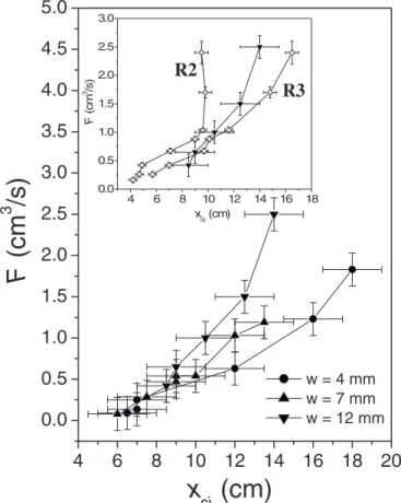
By quantifying the critical length, xci, at which the
transi-tion between continuous and intermittent flow happens, for different input fluxes, we construct the “phase diagram” pre-sented in Fig.10. There, the vertical axis represents the input flux as the volume per unit time of sand added to the cell. As the width of the cell is increased, the transition line increases its slope, indicating that, for a given F, the intermittent flow is reached for smaller piles. The inset of Fig. 10 shows a superposition of the transition line for the case of a Hele-Shaw cell of w = 12 mm and the two lines R2 and R3 corre-sponding to the wide transition to the intermittent regime in the sandpile geometry. The relative position of the lines sug-gests that the revolving rivers can be taken, to a first approxi-mation, as a 12-mm-wide “revolving Hele-Shaw” cell that performs a revolution around the pile at the same frequency of the rivers关1兴. Within this picture, the role of the river is
just to reduce the dimensionality of the flow in the pile. The specific mechanism that triggers the transition from the continuous to intermittent regimes as the size of the sys-tem grows is still unclear for our sandpiles, and also prob-ably for the Hele-Shaw configuration 共we underline that a qualitative explanation is given in 关4兴 for a heap of fixed
length兲. Here we propose an explanation based on segrega-tion. As well known in the case of debris flows in mountains,
bigger rocks tend to accumulate in the flow front as it slides down. This is clearly illustrated, for example, in Fig. 1.4 of Ref.关10兴. Careful inspection of the free surface of our heaps
in the Hele-Shaw configuration also hints at segregation of big grains as we move down the slope, even when our grains are not significantly bidisperse. In fact, the roughness ampli-tude of the surface varies from approximately 0.1 mm to 0.3 mm as we move down the hill共see Fig.11兲. If one assumes
that a slope of bigger grains provides the necessary effective friction to start the growth of a “stop up” front, we speculate that, when the heap, growing to a size large enough for the segregation of big grains near the base, reaches a certain threshold, the intermittent regime is triggered. In analogy, the increase in the radius of the pile is a necessary condition to reach the intermittent regime in the revolving rivers.
V. CONCLUSIONS
We have established experimentally the “dynamical phase diagram” of the continuous and intermittent regimes for re-volving rivers in sandpiles. One somewhat unexpected fea-ture of the diagram is that stable continuous rivers can only exist below a certain input flux threshold: The intermittent regime is the most robust dynamics in the system. The de-tails of the pile shape and of the movement of grains on its surface indicate that, while most of the downhill flow in the continuous regime takes place within the “river itself,” there is a wide area behind it that contributes with much smaller flow. This fact, however, plays a relevant role in the slow change in the slope as one moves around the pile. We have also improved the kinematic model presented in关1兴 in order
to mimic in detail the measured topography of the piles in the continuous regime. The model also allows us to estimate
4
6
8
10
12
14
16
18
20
0.0
0.5
1.0
1.5
2.0
2.5
3.0
3.5
4.0
4.5
5.0
R3
R2
4 6 8 10 12 14 16 18 0.0 0.5 1.0 1.5 2.0 2.5 3.0 F (c m 3/s ) xci(cm) w = 4 mm w = 7 mm w = 12 mmF
(cm
3/s)
x
ci(cm)
FIG. 10. Transition from the continuous to the intermittent re-gimes in Hele-Shaw and revolving rivers configurations. The verti-cal axis corresponds to input volume of sand per unit time, and the horizontal axis is the length of the base of the heap at the transition. The inset shows a comparison between the line of a 12-mm-width cell and the lines R1 and R2 taken from Fig.1.
1 cm 11 10 9 8 7 6 5 4 0.05 0.10 0.15 0.20 0.25 0.30 R o ug hn e s s (mm ) Uphill distance (cm)
FIG. 11. Spontaneous segregation. The graph indicates the de-crease in the roughness amplitude of the pile as we move uphill, suggesting segregation of bigger particles near the lower edge of the heap. The roughness amplitude has been measured as the root mean square of the elevation across 12-mm-long running windows on the free surface seen in the 7-cm-long picture of the lower inset, corre-sponding to the boxed region indicated in the upper inset. We define the uphill distance as the distance from a point on the surface to the top of the pile.
ALTSHULER et al. PHYSICAL REVIEW E 77, 031305共2008兲
the extension of the undulating pattern in the intermittent regime based on other experimental parameters. By perform-ing a series of experiments with Hele-Shaw cells, we con-clude that, due to the reduced dimensionality of the granular flow along the rivers, we can describe them as “revolving” Hele-Shaw cells of 12 mm width—the analogy accounts both for the continuous and the intermittent regimes. Finally, we propose that the segregation of big grains after the pile has reached a critical size is responsible for the appearance of “stop-up” fronts and, consequently, for the transition to the intermittent regime.
ACKNOWLEDGMENTS
We thank H. Herrmann for inspiration in the exploration of new sandpile models, O. Ramos, A. Stayer, and K. Robbie for experimental support, and E. Clément and S. Douady for advice and useful discussions. We acknowledge support from the French Norwegian PICS project, the INSU DYETI pro-gram, the ANR CTT ECOUPREF propro-gram, the REALISE program, the Alsace region, and the Cuban PCNT Grant entitled “Avalanche Dynamics in Physical and Biological Systems.”
关1兴 E. Altshuler, O. Ramos, E. Martínez, A. J. Batista-Leyva, A. Rivera, and K. E. Bassler, Phys. Rev. Lett. 91, 014501共2003兲. 关2兴 X.-Z. Kong, M.-B. Hu, Q.-S. Wu, and Y.-H. Wu, Phys. Lett. A
348, 77共2006兲.
关3兴 E. Martínez, C. Pérez-Penichet, O. Sotolongo-Costa, O. Ra-mos, K. J. Måløy, S. Douady, and E. Altshuler, Phys. Rev. E
75, 031303共2007兲.
关4兴 S. Douady, B. Andreotti, and A. Daerr, Adv. Complex Syst. 4, 509共2001兲.
关5兴 J. Rajchenbach, Phys. Rev. Lett. 65, 2221 共1990兲.
关6兴 P.-A. Lemieux and D. J. Durian, Phys. Rev. Lett. 85, 4273 共2000兲.
关7兴 S. N. Dorogovtsev and J. F. F. Mendes, Phys. Rev. Lett. 83, 2946共1999兲.
关8兴 S. N. Dorogovtsev and J. F. F. Mendes, Phys. Rev. E 61, 2909 共2000兲.
关9兴 Th. Boutreux, E. Raphaël, and P.-G. de Gennes, Phys. Rev. E
58, 4692共1998兲.