Classification of challenging Laser-Induced Breakdown Spectroscopy soil sample data - EMSLIBS contest

(1)

HAL Id: hal-02869477

https://hal.archives-ouvertes.fr/hal-02869477

Submitted on 27 Aug 2020

HAL is a multi-disciplinary open access

archive for the deposit and dissemination of

sci-entific research documents, whether they are

pub-lished or not. The documents may come from

teaching and research institutions in France or

abroad, or from public or private research centers.

L’archive ouverte pluridisciplinaire HAL, est

destinée au dépôt et à la diffusion de documents

scientifiques de niveau recherche, publiés ou non,

émanant des établissements d’enseignement et de

recherche français ou étrangers, des laboratoires

publics ou privés.

Distributed under a Creative Commons Attribution| 4.0 International License

Spectroscopy soil sample data - EMSLIBS contest

Jakub Vrábel, Erik Képeš, Ludovic Duponchel, Vincent Motto-Ros, Cécile

Fabre, Sven Connemann, Frederik Schreckenberg, Paul Prasse, Daniel Riebe,

Rajendhar Junjuri, et al.

To cite this version:

Jakub Vrábel, Erik Képeš, Ludovic Duponchel, Vincent Motto-Ros, Cécile Fabre, et al..

Clas-sification of challenging Laser-Induced Breakdown Spectroscopy soil sample data - EMSLIBS

contest.

Spectrochimica Acta Part B: Atomic Spectroscopy, Elsevier, 2020, 169, pp.105872.

(2)

Manoj Kumar Gundawar

, Xiaofeng Tan

, Pavel Pořízka

, Jozef Kaiser

a_{Central European Institute of Technology, Brno University of Technology, Purkyňova 123, 612 00 Brno, Czech Republic}

b_{Univ. Lille, CNRS, UMR 8516, LASIRe – LAboratoire de Spectroscopie pour les Interactions, la Réactivité et l'Environnement, F-59000 Lille, France} c_{Institut Lumière Matière, UMR 5306, Université Lyon 1 - CNRS, Université de Lyon, 69622 Villeurbanne, France}

d_{Université de Lorraine, Laboratoire GeoRessources (UMR CNRS 7359), 54506 Vandoeuvre-lès-Nancy, France} e_{Fraunhofer Institute for Laser Technology ILT, Steinbachstraße 15, 52074 Aachen, Germany}

f_{Department of Computer Science, University of Potsdam, August-Bebel-Strasse 89, 14482 Potsdam, Germany} g_{Physical Chemistry, University of Potsdam, Karl-Liebknecht-Str. 24-25, 14476 Potsdam, Germany}

h_{Advanced Centre of Research in High Energy Materials, University of Hyderabad, Prof C R Rao Road, Central University Campus PO, Gachibowli, Hyderabad, 500046,} Telangana, India i_{X Scientific, China} A R T I C L E I N F O Keywords: EMSLIBS contest Chemometrics

Laser-induced breakdown spectroscopy (LIBS) Machine learning

Classification benchmark

A B S T R A C T

We present results of the classification contest organized for the EMSLIBS 2019 conference. For this publication, we chose only the five best approaches and discussed their algorithm in detail. The main focus of the contest reflected both recent and long-term challenges of Laser-Induced Breakdown Spectroscopy (LIBS) data proces-sing. The contest was designed with a purpose to raise a challenge in handling and processing a very large dataset, containing high-dimensional elemental spectra. For the contest, 138 samples were measured using a lab-based LIBS system. In total, the data set consisted of 70,000 spectra, separated into 12 classes according to their elemental composition. Due to its extensivity and complexity, the data set is unique within the LIBS community. The central idea was to simulate the so-called “out-of-sample” classification (i.e. according to similar elemental composition), implying various real-world applications. Even more, it reflects the current level of expertise in the LIBS community and the capability of the LIBS method itself.

1. Introduction

Laser-induced breakdown spectroscopy (LIBS) [1,2] is a semi-quantitative analytical technique suitable for fast elemental analysis. LIBS became a widely used method in a variety of applications, e.g. the industrial analysis of metals [3], mining purposes [4], forensic analysis [5,6], elemental mapping of biological samples [7–9], analysis of mi-nerals in geological research [10–12], and most prominent - space ex-ploration [13]. Many improvements have emerged in recent years as a result of technological progress. Notably, the speed of analysis has dramatically increased (up to 1 kHz [14]), which allowed the mapping

of extensive areas. Also, necessary equipment (pulsed laser, spectro-meter) is more accessible and robust, allowing to create cheap, portable and modular LIBS devices.

A significant milestone that increased the method's analytical cap-abilities was the incorporation of modern data mining [15,16] and machine learning [17] approaches to LIBS spectra processing. Espe-cially, for the advanced analysis of large, high-dimensional datasets (e.g. originating from elemental mapping or the ChemCam device [13]), it is not manageable to use common simple statistical explora-tion. However, the introduction of modern data processing techniques to LIBS was turbulent and a unified direction (or consensus) is still

https://doi.org/10.1016/j.sab.2020.105872

Received 31 January 2020; Received in revised form 29 April 2020; Accepted 30 April 2020

☆_{Selected Paper from the 10th Euro-Mediterranean Symposium on Laser-Induced Breakdown Spectroscopy (EMSLIBS 2019) held in Brno, Czech Republic, 8–13th} September 2019.

⁎_{Corresponding author.}

E-mail addresses:[email protected](J. Vrábel),[email protected](L. Duponchel),

[email protected](F. Schreckenberg),[email protected](P. Prasse),[email protected](M.K. Gundawar),[email protected](X. Tan). 1_{These authors contributed equally to the work.}

Available online 05 May 2020

(3)

missing. Thus, the performance comparison and consequent stabiliza-tion of selected techniques would be beneficial for the community and for the further evolution of the analysis.

In the past, two public contests were launched inside the LIBS community. Both of them were organized by Dr. Igor Gornushkin - BAM (GE). The task of the contests was to quantify selected elements inside a few unknown samples by using knowledge obtained from “training” samples with provided compositions. Results of these contests were presented at conferences. It is worth mentioning that one more com-parative contest of the French LIBS community [18] was held. In this contest, only data were shared to participants in order to exclude ex-perimental factors from the comparison of quantification approaches.

In order to continue with this tradition, we decided to create a classification contest as a part of the EMSLIBS 2019 conference. We have created a challenging task covering both recent and long-term problems appearing in LIBS spectra processing. The main task of the contest was to correctly classify the highest possible number of un-known spectra (Test dataset) using the information provided by labeled spectra (Training dataset).

Inspired by general machine learning, we designed a dataset that required a model with the ability to generalize well. This means that a classification model, learned on a specific sample set (e.g. personal cars vs. planes), is able to be generalized over the training data (extract only important features) to enable the classification of the distinct sample sets (e.g. trucks vs. cargo aircraft). Transferring this idea to spectro-scopy; a model is trained on a set of spectra originated from minerals (e.g. various hematite samples) with varying elemental composition (in a feasible range). Then, the goal is to classify spectra from an entirely new physical sample (but still geologically labeled as hematite). The presented task is also a good simulation of the real LIBS application, used for instance as a trash separator [19]. Such a device should be able to correctly separate even contaminated specimen (e.g. dirty glass bottles), where the measured spectrum is affected by the pollutant.

In this manuscript, we present details of the contest as well as the approaches of five best teams that participated in the competition. We believe that the presented results will shed light upon the actual state of data processing carried out by individuals of the LIBS community (considering analytical performance) and stimulate collaboration among groups.

2. Contest description

One of the most frequent applications of LIBS is material identifi-cation. Since most of these tasks are carried out based on a material library, they can be regarded as a classification. Hence, this competition aims to find a robust classification algorithm capable of dealing with challenging datasets. The goal of the competition is to classify the test dataset with the highest possible classification accuracy.2

2.1. Motivation

Supplied by a sufficient amount of data, modern machine learning methods are able to learn the distribution of LIBS spectra accurately. Therefore, the classification of samples (or spectra) selected from the same probability distribution is generally highly successful and poses no real challenge. Nevertheless, in real-life applications, a set of samples is usually available for training, while the classification is targeting a wider range of samples: mineral samples, such as hematites (e.g., several he-matite samples can be collected and used to build a classification model which is later used to identify a wider range of hematite samples); me-tallic materials contaminated with various pollutants, etc. Hence, the dataset subject to this competition simulates these conditions.

2.2. Design of the contest

While designing the contest, we kept in mind a few essential ideas to be incorporated into the task. As already mentioned, the so-called “out of sample” classification was the cornerstone of the contest. To make it possible, a large number of samples and measurements had to be pro-vided, allowing the usage of advanced data processing techniques. A large number of spectra to analyze restricts the possibility of exploring each spectrum by hand, using standard spectroscopic expertise. However, an incorporation of such expertise during the preprocessing or results evaluation is still beneficial. The key is to find a balance between spectroscopy and “blind” data processing.

2.3. Samples and data

The contest dataset with the accuracy feedback is accessible on the webpage [20] and details at [21].

A brief summary of the size and composition of the data set:

•

138 samples

•

12 classes

•

500 spectra per sample (in training dataset)

•

20,000 spectra in test dataset (in total)

•

40,002 wavelength points per spectrum

The samples were OREAS (ORE Research & Exploration Pty Ltd., AU) certified soil powders cast into gypsum for more convenient handling. There were 12 classes in total, consisting of 138 physical samples. However, the number of samples varied among classes. For each sample in the training dataset, there were 500 spectra available, with corresponding class labels. The division of dataset to training and testing part was made according toFig. 1. In one class (e.g. Hematite), there were n samples with a similar chemical composition. However, specific concentrations varied in some range, so the resulting spectra were different. Two thirds (⅔) of all samples were physically produced as a mixture. For every mixed sample, we took ¾ of its weight from one “original” material (Oreas powder) and mixed it with ¼ weight of randomly selected material (distinct Oreas powder). The remaining part of the samples (1/3) were made of pure material (Oreas samples).

A more detailed description of the samples, measurement conditions and raw data can be found in [21].

2.4. Rules

Participation in the contest was conditioned by the following rules:

•

Contestants were free to form groups as long as they were registered as such, i.e., individual groups were requested to participate using a single account;

•

Collaboration among separate groups was discouraged;

•

Contestants were free to process the spectra as they saw fit;

•

In addition to the behaviors outlined by the official competition

rules, “forbidden behavior” encompassed any attempt to gain an edge in accuracy by using information that was outside of the pro-vided dataset, or an attempt to use the propro-vided information in a way that was not intended. Examples of forbidden behavior in-cluded (but were not limited to):

•

Attempting to use datasets and references beyond those made available by the competition;

•

Attempting to abuse the competition infrastructure to gain an edge. 2_{Classification accuracy (or just accuracy) is defined as number of correct}

(4)

3. Approaches of participants

3.1. Ludovic Duponchel, Vincent Motto-Ros, Cécile Fabre (referred as LD team)

The development of a classification model is a time-consuming task because it requires many steps. From the very beginning of our parti-cipation in this challenge, we quickly discovered that the dataset was special because it consisted of a very large number of spectra. Moreover, the developed model also had to manage a large number of mineral classes. A real challenge was ahead.

3.1.1. Data preprocessing

Based on this observation, we first decided to reduce the number of spectral variables in the data set using a simple procedure of length down-sampling. In fact, emissions at three consecutive wave-lengths were replaced by a single one considering their mean thus re-ducing the number of spectral variables by a factor of 3. It was also a good way to suppress potential spectral shifts and to increase a little bit the signal to noise ratio. In order to reduce the matrix effect, a nor-malization was used fixing the total area of spectra equal to one. Concerning the spectral domain, our strategy was to keep all available information in the data set. Consequently, no emission lines selection had been considered prior to chemometric explorations. Lastly, a gap-segment derivative was applied to spectra in order to suppress potential baseline drifts. This technique is first based on smoothing the spectrum and then calculating signal differences over successive wavelengths considering a gap between them. Interested readers will find more details about this derivative in the article by K·H Norris et al. [22].

3.1.2. Classification model design, further data processing

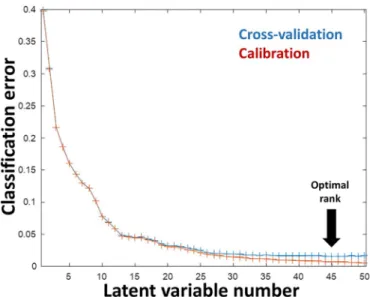
Our objective has been first to develop a classification model using a classical and well-known algorithm called partial least squares dis-criminant analysis (PLS-DA). Such as the PLS regression used for the prediction of continuous values, a PLS-DA model requires an optimal number of components for the considered data set. In our case, venetian blind cross-validation has been used in order to select the optimal number of PLS components. Fig. 2 depicts the evolution of the

classification error depending on the number of components during cross-validation. The lowest cross-validation classification error is then observed for a PLS-DA model using 45 components (black arrow).

However, we notice that this optimal number of components is huge compared with the 12 classes to be predicted, which is really unusual for this kind of algorithm. With this classification model, we observe a classification rate of 99% on the training data set and only 76.64% on the test set. The classification rate is the percentage of well-classified samples relative to all samples in the dataset. Such a decrease is of course not acceptable and reflects a situation for which the training and test sets are not representative of each other. In other words, we try to classify new spectra which have not really been observed during the training step. Our objective being to propose the best predictive model, we have then to understand where these differences are and to try to correct them in the second step in order to increase the classification rate.

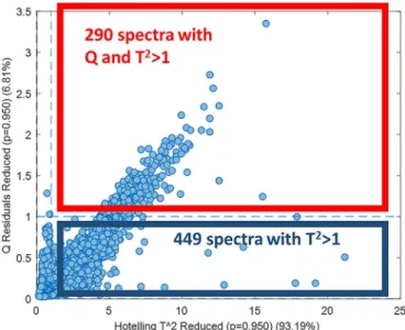
In chemometrics, it is usual to use statistical tests in order to highlight potential outliers, i.e. spectra observed out of the hyperplane defined by the considered model. A Q/T2_{plot is then considered giving} the Q contribution and Hotelling's T2_{values for each spectrum of a data}

Fig. 1. Representation of a selected class in artificial parametric space. The

subclass is a collection of spectra measured from an identical physical sample.

Fig. 2. (left). Optimization of the model complexity during the cross-validation

step.

Fig. 3. (right). A Q/T2_{plot of the training and test sets. The red circle highlights} 509 spectra of the test set (gray dots) having specific spectral contributions (not seen in the training set i.e. colored dots).

(5)

set. Fig. 3presents such a graph with training (calibration) and test samples highlighted in colors and gray respectively. It is obvious that 509 test spectra (circled in red) with Q and T2_{values higher than 1 are} the worst outliers because they are completely far and/or out of the hyperplane defined by the classification model. These spectra are really inconsistent with the ones observed during the training.

In order to find potential spectral differences between these 509 spectra and the others, a principal component analysis (PCA) has been developed with all spectra of the training and test sets simultaneously. Fig. 4shows different scores plots with specific 509 spectra colored in light blue and the other spectra of the training and test sets in dark blue. It is then easy to see that the 18th principal component (PC18) mainly explains these spectral differences.

Indeed, looking at the PC1-PC18 score plot, it is obvious that the 509 spectra in light blue exhibit significant positive scores along the 18th principal component (PC18) which is not the case for the rest of the samples. As this spectral contribution is absent in the training set, the idea was to suppress it in the test set reconstructing test spectra with a classical linear combination of scores and principal components without PC18, a total of 200 principal components being considered in the reconstruction. Considering these new corrected spectra in the test set, a real benefit of this filtering was observed with 78.235% of good classification. The prediction was thus improved but it was still not enough compared with the 99% training rate. With this new model, it was possible to explore again the Q/T2_{plot presented in}_{Fig. 5}_.

3.1.3. Final model

A new set of 739 test spectra have been again considered as outliers (i.e. non representative of the calibration data set). Specifically, 290 samples had values of Q and T2_{greater than 1 and another 300 had only} the value of Q greater than 1. However, it was impossible this time to observe specific contributions for those specific spectra compared with the whole dataset using the previous PCA filtering trick. Therefore, we had to find another strategy. When a PLS-DA model is used to predict class membership from a spectrum, we obtain one probability of membership for each class. The probability of the corresponding sample to belong to a given class. These probabilities being independent, we

can thus expect that a given sample may present a very high probability for a given class but even a very low probability for the other classes. Looking at these probabilities for this new set of outliers, we have discovered that almost all of them had simultaneously probabilities of membership very close to one for classes 6, 7, and 11. There was therefore an ambiguity of prediction between these three classes for the outliers considered. Of course, the algorithm selected for each sample the highest probability but there was potentially no significant differ-ence between the probabilities of the three classes. As a consequdiffer-ence, these samples were almost systematically predicted as class 6 which was certainly not a good thing given the prediction results. The next idea was then, for each of the (209 + 449) spectra, to decompose it using a non-negative least-squares procedure considering the mean spectra of all training samples belonging to classes 6,7, and 11. In this

Fig. 4. A PCA exploration highlighting a significant difference along PC 18.

Fig. 5. (left). The new Q/T2_{plot considering the classification model with} corrected spectra. Only test spectra are presented in the figure.

(6)

way, three weighting coefficients consistent with these three classes were obtained for each outlier sample. Then the highest weight ob-tained from such a decomposition on a spectrum has given the class of the corresponding sample. Then we have discovered that most of these samples were reassigned to class 11 when they were mostly predicted 6 initially. The effects of this new strategy were not long in coming, as the new classification rate on the test set was 80.365%. In order to go even further, an original approach was then tried. In fact, we developed a PLS-DA model with the test set as a training (calibration) set and re-ference labels were obtained later on (with a classification rate of 80.365%). An optimal model had 34 PLS factors and the use of the same data set as validation one allowed us to reach a classification rate of 83.57%. In the next step, a new Q/T2_{plot of the model enabled us to} discover more than 2000 spectra having simultaneously Q and T2 va-lues higher than one (Fig. 6). Again, for these detected spectra, a nonnegative least-squares decomposition was applied. In fact, many of these samples were reassigned to classes 11 and 1 giving the final classification rate of 90.33%.

3.2. Sven Connemann Frederik Schreckenberg (referred as ILT team)

The Fraunhofer Institute for Laser Technology ILT has great ex-pertise in spectroscopy. Naturally, our approach for classification of the EMSLIBS contest dataset is based on this expertise rather than machine learning algorithms.

3.2.1. Data preprocessing, feature engineering

The used classification approach is mainly based on the idea of calculation of equipment ability indexes to separate classes. The equipment ability index can be calculated for every test data input feature, meaning for every wavelength step of the spectra. The equip-ment ability index spectra cij(λ) between class i and class j is defined as:

= + c ( ) I ( ) I ( ) 2( ( ) ( )) ij i j i j (1)

where Ii are the average spectra of each class, and σi their standard

deviation.

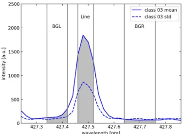
Based on these informations, regions of interest can be chosen for further analysis. Each region of interest contains at least one emission line. The region of interest intensityIROIis calculated with integration over a wavelength area, where the emission line is, and the subsequent correction of a linear background by subtraction of integrated

wavelength areas near the emission peak. The procedure is illustrated below, in gray the areas of the left background (BGL), emission line (Line) and right background (BGR) are marked. The region of interest (ROI) intensity is then calculated as follows:

= +

IROI Il IBGR l BGL I , BGR BGL BGL

BGR l

BGR BGL (2) where Ilis the area of the line emission peak (Fig. 7, gray area labeled

Fig. 6. (right). Q/T2_{plot of the PLS-DA model. Only test spectra are presented} in the figure

Fig. 7. Graphical illustration of the integration areas used to determine the

intensity of an ROI. The shown spectrum (mean) and its standard deviation (std) are from class 03 of the contest training data. The intensities used to calculate the ROI intensity are the gray areas, the edges of the corresponding wavelength areas are marked as gray lines.

Table 1

List of ROIs.

Background left Peak Background right Left [nm] Right [nm] Left [nm] Right [nm] Left [nm] Right [nm] 308.500 308.720 309.160 309.420 309.640 309.780 325.820 326.080 326.220 326.280 326.380 326.520 327.180 327.320 327.380 327.440 327.540 327.700 331.420 331.960 334.360 334.760 335.580 335.920 352.240 352.380 352.440 352.500 352.760 352.900 360.080 360.140 360.500 360.600 361.400 361.620 383.500 383.560 383.760 383.880 383.960 384.020 393.920 394.080 394.320 394.560 395.000 395.240 402.400 402.880 403.280 403.360 403.700 404.040 405.040 405.280 405.740 405.860 406.540 406.660 425.460 425.720 426.040 426.140 426.420 426.780 427.340 427.420 427.460 427.520 427.640 427.760 453.040 453.220 453.300 453.620 453.800 454.200 454.620 454.820 455.340 455.520 455.880 456.140 479.060 480.080 480.840 481.320 481.440 481.560 481.620 482.060 482.260 482.440 482.800 483.240 492.860 493.060 493.340 493.520 494.100 495.000 495.220 495.480 495.740 495.820 496.280 496.560 498.880 499.020 499.080 499.180 499.300 499.420 499.560 499.740 499.900 500.020 500.320 500.460 517.700 518.140 518.340 518.440 518.640 518.760 520.720 520.760 520.800 520.940 521.160 521.260 522.160 522.480 522.660 522.800 523.860 524.080 531.700 531.960 532.060 532.180 532.240 532.320 723.620 724.440 725.880 726.080 727.180 727.740 763.220 764.320 766.000 766.460 768.160 768.360 773.480 773.660 773.940 774.060 774.840 775.340 779.100 779.500 779.960 780.160 780.540 781.120 792.140 793.480 794.680 794.860 795.880 797.280 817.740 817.900 818.260 818.520 818.940 819.120 851.140 851.780 852.040 852.200 852.420 852.780

(7)

Line), IBGRis the area of the right background (Fig. 7, gray area labeled BGR), IBGLis the area of the left background (Fig. 7, gray area labeled BGL), λlis the mean wavelength of the line area, λBGL is the mean wavelength of the left background area and λBGRis the mean wave-length of the right background.

Based on the cij(λ) spectra, for all class pairs, 31 regions of interests

were chosen for the whole training data set (seeTable 1for List of ROIs below). The regions of interest with the largest civalues are chosen for

the following classification task. All chosen regions were manually verified to ensure the presence of a line emission peak and to avoid overlap of the chosen peak with other line emission peaks which are present in the training data set. Also regions of interest with other line emissions in the background areas were neglected. These 31 features were extracted in every single spectrum. Each feature set is scaled to its root mean square (RMS) value. The whole dataset is standardized so every feature has a mean value of 0 and a standard deviation of 1.

3.2.2. Classification model design

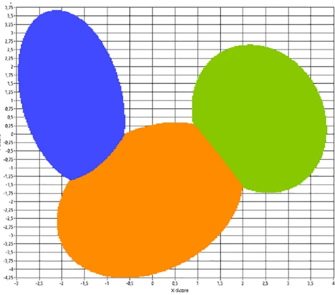
A linear discriminant analysis (LDA) for each class (one vs. all other classes) was calculated. Also, an LDA for each possible class combina-tion was calculated. Via the one vs. all other classes LDAs, the most separable class combinations (with 2 or more classes) are chosen. To improve classification, additional LDAs with only these classes (see Fig. 8for an example LDA of the classes 4, 5, and 6) were calculated.

In the projection of the data in all LDA spaces, class boundaries are

defined as lines of constant Mahalanobis distance to the class data point distribution average (seeFig. 8, ellipsoids around data point distribu-tion). Where class boundaries overlap an equal Mahalanobis distance to both class averages is defined as a class boundary (seeFig. 9, class boundaries marked in blue, orange and green).

The preprocessing of the test data bases on the training data ana-lysis. The same 31 features are extracted for every test spectrum. All features of one spectrum are referenced to its root mean square. To standardize the test spectrum the previously calculated transformation of the training dataset is used.

The test data of each preprocessed spectrum is transformed to the LDA spaces. This leads to one data point per measurement and LDA space. If this data point is in all LDA spaces within the previously computed boundaries of the same class the measurement data is as-signed to this class. This approach can also result in a not valid clas-sification for one spectra. In these cases the clasclas-sification decision bases on the minimal mean Mahalanobis distance of the classes.

With this approach, the ILT team reached 83.14% accuracy on the test dataset and 81% accuracy in the one-shot classification test.

3.3. Paul Prasse, Daniel Riebe (referred as PP team)

Developing a classification model for a problem setting where the

Fig. 8. (left). Example of the projection of the 2 dimensions of the data in LDA space. The LDA is calculated with the data from classes 4 (blue), 5(orange), and 6

(8)

training and test sets differ from each other and the inputs are spectra is challenging. We had some experience working with spectra in another project, so we wanted to test, whether our approach of using a neural network can compete with the state-of-the-art in this field.

We implemented different feature sets. Some include handcrafted features and some implement features created using an autoencoder/ dimensionality reduction scheme [23,24]. This is the list of features used in the final model:

1. manually created features, referred to as [manual]: A feature vector

consisting of the mean, median, standard deviation, and other measurements for different windows of the given spectra (window size of e.g. 100 units with a stride of e.g. 100 units over the se-quence) was created. Before applying this feature extraction, each spectrum was normalized to have a minimum value of 0 and the maximum value of 1 (MinMax Normalization). This results in a vector of 14,035 features.

A detailed list of extracted features per window (of size 100) is the following:

- Mean, median, standard deviation

Fig. 9. (right). The same projection as isFig. 8, but here the class boundaries, defined by equal Mahalanobis distance are shown.

(9)

- 10th percentile, 20th percentile, …, 90th percentile

- Minimum value, maximum value, minimum id, maximum id, - Number of intensities over 20 uniformly selected thresholds in the

range from 0 to 1

- Minimum value, maximum value, minimum id, maximum id 2. features created by autoencoder, referred to as [auto]: We trained an

autoencoder [23] that tries to reconstruct the original sequence from a lower-dimensional representation. Simple Feed-Forward ar-chitecture for the neural networks (NN) proved sufficient as more sophisticated architectures such as long short-term memory (LSTM) [25] and convolutional neural networks (CNN) [26] performed much worse.

An autoencoder (seeFig. 10) was trained for different sizes (8,16,32, …,4096) of the internal embedding (number of units in the dense final layer). The final representation was created by combining the internal representations of the trained autoencoders. This results in a representation of 8184 features for each sequence.

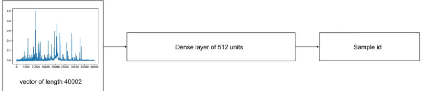
3. Downsampling, referred to as [down]: The input data was sampled down by computing a moving average using a sliding window of size k and stride size of k over the original sequence. In the final model, a combination of the downsampling results for k = 4 and k = 8 was used (e.g. four or eight points are aggregated together, respectively). 4. Classifier able to identify the sample based on a spectrum, referred to as [sample]: A classifier that is able to classify each spectrum according to the sample it comes from. Subsequently, a uniform manifold approximation and projection (UMAP) dimensionality re-duction was applied to the internal representation (output of the dense layer with 512 units) in order to reduce the dimensionality to 100. This resulted in a feature representation of 100 features. (see Fig. 11) [24].

5. UMAP dimensionality reduction applied to the spectrum, referred to as

[UMAP]: A UMAP embedding of the original input (vector of 40,002

entries) was performed and 100 dimensions were retained. This results in a feature representation of 100 features [24].

The following architecture (Fig. 12) was used for training the NN: The different feature embeddings are provided as the input of the neural network (NN). Then, the inputs were fed into a dense layer in order to reduce the dimensionality. Subsequently, all the embeddings were combined in a concatenate layer. This resulted in a one dimen-sional vector that was further processed by a number of fully connected layers. The last layer was a softmax layer producing the final output. This layer is used to classify the given input into the classes.

The final model configuration (weights for the NN) was obtained by the following pipeline:

1. A train test split of the entire training dataset was created. To that end, one specific sample from each class was selected for the test set. All remaining samples were used for training. Thus, the evaluation framework evaluates how the models perform on unseen samples. In this way, it is possible to estimate how well each model is able to generalize to new unseen samples and to avoid overfitting. 2. A random set of input features (out of 5 feature sets) was selected as

the input for the neural model. This could be only one feature set, all the feature sets, or a subset of all features sets.

3. A random number of dense layers (1,2, or 3) and a random number of units for the dense layers (8,16,32,64,128,256,512,1024) was chosen.

4. A large number of models were trained and evaluated on the in-ternal test set.

5. For each model, the validation accuracy (percentage, showing, how often the models correctly predicts the correct class) and the cross-entropy loss on the internal test set were stored.

Using this pipeline, the predictions on the competition test set using the k (14 for the competition) best performing models on the internal test set were stored. The single best performing model consists of 3 dense layers with 64 units each. These k predictions were combined by performing major voting, where the number of models voted for the

Fig. 11. The architecture of the classifier.

(10)

entire training data plus the instances where at least x models agreed on the classification of test set samples. Thus, a model was trained on the training and testing data of the competition. It was observed that models trained this way had performed much better than models only trained on the training set.

3.3.4. Results

The evaluation was carried out for the model trained solely on the training data and the one additionally containing the instances from the test data upon which at least x, x-1, x-2 (14,13,12) models agreed. The average results for 10 different initializations of the NN using the best parameters found for the numbers of dense and hidden units are the following (the results show the average accuracy with corresponding standard error):

•

accuracy for the model only trained on the training set: 67.68% + − 2.29%

•

accuracy for the model using the training set and 16,220 instances from the test set (14 models agree): 81.22% + − 0.96%

•

accuracy for the model using the training set and 17,595 instances from the test set (13 models agree): 80.876% + − 1.22%

•

accuracy for the model using the training set and 18,295 instances

from the test set (12 models agree): 81.04% + − 0.62%

3.4. Rajendhar Junjuri, Manoj Kumar Gundawar (referred as MKG team)

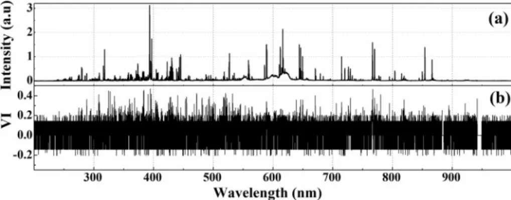
Our approach was based on various feature selection methods, which were employed to reduce the overall size of the input data before classification. The methods included - peak-find using an algorithm, manual-peak find and random forest (RF) algorithm. The spectra were first normalized at 714.84 nm (this line was selected after visual in-spection), as shown inFig. 13a before performing the analysis.

First, an algorithm developed in MATLAB was used for feature se-lection. This algorithm is based on a moving window approach with width and height being the parameters. A total of 1278 peaks were detected using this approach. The intensity at the peak center (variable at peak maximum) was considered as a feature. This corresponded to

Further, the peaks were also manually selected by visual inspection. Initially, a spectrum for each sample was generated by averaging the total number of spectra available for that sample. Later, the spectral features were systemically selected from the entire spectra based on their intensity. A threshold intensity value of 0.005 was chosen for the feature selection. Thus, only the spectral lines with higher intensity than the threshold were considered for the analysis. This approach provided 15,085 variables for the classification.

Lastly, a multivariate method, an ensemble-based decision tree al-gorithm i.e., random forest (RF) [27] algorithm was employed. It pre-cisely finds the pattern buried in the input data that replicates the useful information by properly guiding and training through supervised learning which is not possible by manual inspection. It is a bootstrap aggregation method where a different number of trees is grown based on the application of interest. The trees in RF grow independently and randomly by selecting the bootstrapped dataset. Further, each tree is grown by selecting a variable and corresponding error/impurity is es-timated. The error is calculated by measuring the information gain (IG). Further, the variable importance (VI) is estimated by the sum of the decrease in error when split by a variable (for details see [27]) For the present investigation, 50 trees were considered and further, the features were selected based on variable importance (VI) of the trained RF model as shown inFig. 13b. The variables of high importance had a significant effect on classification. Error prediction was based on out of bag observations and the minimum number of observations per tree leaf was one.

The lower values of VI does not influence the predictive ability of the analytical technique and are omitted from the analysis. The features are selected by varying the threshold value of the VI. For example, the threshold value 0.01 represents only the variables with VI greater than 0.01 are considered. For the present study, three values of VI viz., 0.01, 0.1 and 0.2 have been considered, which resulted in obtaining the 9720, 9140 and 1379 features, respectively.Fig. 14represents the LIBS spectra (black line in the range of 400–450 nm) with superimposed features (red dots) selected using the RF algorithm. Only a 50 nm spectral window is shown for better visualization of the selected fea-tures.

Hence, in total five different types of sets of features were selected. The first two belong to peak find algorithm and manual feature

Fig. 14. The LIBS spectra of sample 1 in the spectral

window of 400–450 nm. The red dots represent the features VI > 0.2. (For interpretation of the refer-ences to colour in this figure legend, the reader is referred to the web version of this article.)

(11)

selection respectively and the last three are based on RF algorithm.

A three-layer neural network algorithm with a feed-forward back-propagation approach for labeling the samples was employed. The number of neurons in the hidden layer varied from 20 to 50 in steps of 5 for optimizing the performance of the network. Cross entropy was se-lected as a cost function. Forty neurons were found to be optimal in all the models. The training dataset (training set given to us) was divided into three sets viz., training, validation, and testing in the proportion of 60, 20, and 20%. The analysis was repeated ten times where the training, validation, and testing datasets were randomly divided and ten different artificial neural network (ANN) models were established.

The feature selection was performed on the training dataset in dif-ferent ways as aforementioned. An ANN model was then applied using these features as input. The model was optimized for number of neurons based on the test data accuracy. For each type of input feature, the testing was performed using ten different models obtained by randomly dividing the training dataset into training, validation, and testing. The accuracy is reported as an average of these ten iterations. The un-certainty refers to the standard deviation of the correct classification rate calculated over ten iterations. Finally, the model which resulted in maximum accuracy for each type of feature, except the peak-find al-gorithm, was considered. The label of the test data was then decided by voting among the four labels.

3.4.4. Results

•

The accuracy obtained from the model trained with the peak-finder program is 61.95 ± 0.73.

•

The accuracy obtained from the model trained with manual feature selection is 72.18 ± 1.08.

•

The accuracy obtained from the model trained with spectral features with VI > 0.01 is 75.14 ± 0.86.

•

Finally, the accuracy of 77.89 was achieved by voting among the best from the last four models (2–5).

3.5. Xiaofeng Tan (referred to as XT)

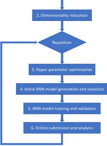
I have approached the challenge in a typical machine-learning workflow: data preprocessing, model building, modeling training and validation, and model prediction. Our approach is shown in the sche-matic diagram inFig. 15.

3.5.1. Data preprocessing

Steps 1 and 2 of the method are meant to reduce the dimensionality of the Training and Test datasets employing PCA. The PCA is performed on the Test dataset (instead of larger Training dataset) to reduce the computational cost of the process. Before the PCA, a signal-to-noise-ratio (SNR) estimation of the Test dataset with the Beta-Sigma proce-dure [28] is performed. The dimensionality reduction of both Training and Test datasets is achieved by calculating the PCA scores of the data using only the first PCA components whose accumulative percentage variance is higher than 1–0.67 / SNR, where SNR is the value de-termined in Step 1. This way, we reduce the dimensionality of both the Training and Test datasets from 40,002 points in the original spectral space to 13,705 points in the truncated PCA space.

An ANN is used in our model for modeling the Training dataset and

for predicting the Test dataset. More specifically, a feed-forward mul-tilayer perceptron (MLP) with the rectified linear unit (RELU) and the Softmax activation functions for the hidden dense layers and the output layers, respectively, was used to model the data. Each hidden layer is followed by a dropout layer in the MLP, a technique commonly used in ANN to prevent overfitting [29]. In Step 3, various model hyper-para-meters such as number of hidden layers, numbers of nodes in the hidden layers, L2 regularization, dropout value, maximum kernel norm (MKN), and training parameters such as numbers of batches and epochs are either chosen based on experience and memory limitation of our computer system (in the first run) or adjusted from previously chosen values (in the successive runs) based on model performance. In training, the original Training dataset is further split into model training (MT) and model validation (MV) datasets with a 9:1 ratio. The MT dataset is used to train the model, and the MV dataset is used to check the pre-dicting power of the trained model.

In Step 4, a number (e.g. 30) of “initial” ANN models of the same MLP structure are generated with randomly generated initial weights and biases and are trained with the MT set for only 100 epochs. The best performing model is then selected from the initial models based on their prediction accuracies with the MV set. The purpose of this step is to identify the best random initial parameters that likely lead to the best performing model of the given MLP architecture at a minimal compu-tational cost. The full training is carried out in Step 5 with the selected best performing initial model and with the MT dataset. Once the model is trained, its prediction accuracy is checked with the MV dataset. In Step 6, the fully trained model is used to predict the original Test da-taset and the prediction is submitted online to determine the prediction accuracy. Based on the reported online accuracy the model hyper-parameters are adjusted manually and Steps 3 through 6 are repeated until no visible improvement on the reported accuracy can be achieved.

(12)

The best performing model produced from the above steps contains a single hidden layer with 512 nodes with the following model para-meters: a dropout value of 0.2; the MKN value of 2.5; a training batch size of 1000. In the model training process was observed that our ANN models consistently achieved >99.95% prediction accuracy with the MV dataset that was not included in the training. However, even the best performing ANN models that we produced achieve only (76.78 ± 0.56) % accuracy for the final Test dataset. We speculated that the Test dataset contains patterns that are not present in the training dataset. This speculation is identified and confirmed in the approach of the LD team.

4. Discussion and results

This work presents five unique approaches applied to a challenging classification task. Conventional methods (PCA combined with ANN or feature selection prior to ANN) led to a respectable accuracy. However, for reaching top edge results, the incorporation of original ideas into the data processing pipeline was required. Here, we (organizing team from CEITEC BUT) present our opinion and the summary of key ideas of each presented approaches.

By each participating team, feature selection (or dimension reduc-tion) techniques were employed. Later, for the final classification, a variety of machine learning techniques was utilized with essential dif-ferences.

XT reduced the original dimension by standard (but effective) PCA. As a classifier, feedforward ANN was used. The slightly unconventional approach where the PCA model was built on the test data, was limiting the classifier's ability to generalize. This resulted in a rapid decrease in the accuracy of the “one-shot” attempt, realized after the contest.

The MKG team focused preferably on feature selection, using both manual and automatized peak finding (or selection), and also a random forest (RF) algorithm. RF has been proven useful for the extraction of important spectral features. Again, feedforward neural network classi-fiers were built on selected feature sets (one model per feature selection (FS) technique) and the final label was selected by a voting scheme.

The PP team brought the most up-to-date machine learning tech-niques and a very solid (and educational) methodology into the contest. Several FS techniques (manual selection, autoencoder, down-sampling, UMAP, classifier NN) were employed together in a connected pipeline leading to a feedforward neural network classifier. Splitting of the training dataset was done in a sample-wise way, exactly respecting the task of the contest and extending model generalizability. Utilized FS techniques in the pipeline were selected randomly, resulting in many distinct models that were trained. Before the final step, test spectra had been classified by 14 models. “Easily classifiable spectra” (where most of the models agreed upon the class) had been transferred from a test (unknown) dataset to an extended train (known) dataset. The final model was trained on this extended training dataset and used for

The ILT team used a more “spectroscopic” approach to data pro-cessing. Regions of interest in spectra were chosen, using equipment ability indexes in order to separate classes. This elegant (and spectro-scopically explainable) technique allowed them to obtain a set of only 31 features for LDA used as a classifier. Even while LDA is a relatively simple classification technique, it obtained excellent results in the contest, supported by properly selected features. This also implies the preserving importance of spectroscopic expertise in processing of spectroscopic data, assisting to modern data mining approaches.

Finally, the winning LD team used a variation of the “spectroscopic” approach as well. A lot of time was spent on a detailed exploration and understanding of the data. Differences between training and test data-sets (as explained in the contest motivation) were detected and studied deeply. A statistical test (Q/T2_{plot) was used in order to find the most} differing spectra among the dataset. Consequent analysis of a PCA model discovered that the contribution of the 18th principal component had mostly been responsible for the mentioned difference of spectra and had been suppressed later in the reconstruction of the data. This step improved the classification accuracy of the used PLS-DA model. Problematic data classes in the model were detected and a part of spectra was reassigned according to a non-negative least-squares pro-cedure on the mean spectra of class. At that point, the key idea (similar to the PP team) was realized. PLS-DA model was built on training data, also using the test (initially unknown) data as validation, with labels obtained from classification in the previous step. In contrary to results from other teams, only this approach was able to pass the 90% classi-fication accuracy with a considerable edge.

It is worth mentioning that using information from (or handling with) the test dataset during the design of the classification model could be sometimes considered as a restricted move. This was of course vio-lated by several participants, as was described above. However, in this contest, such behavior was NOT restricted by the rules and thus was completely acceptable. Even more, it makes sense from the spectro-scopic point of view to consider possible applications such as the mentioned trash separator. In the real-world application, continuous improvement of the model is advisable.

4.1. One-shot classification

After the contest, an additional test dataset was released. It con-sisted of different measurements from identical samples of the “original “test dataset. For this new dataset, no feedback accuracy was provided, and participants had only one attempt for result submission. Thus, it serves as confirmation for the robustness (generalizability) of the model. In the result table (Table 2), we provide this one-shot accuracy for selected participants. Unfortunately, the LD team had not partici-pated in this additional one-shot confirmation due to lack of time.

(13)

5. Conclusion

In this manuscript, we present a report of the spectra classification contest which was organized as a part of the EMSLIBS 2019 conference. The task of the contest was to classify an extensive and challenging LIBS dataset with the highest possible accuracy. Feedback with current ac-curacy was automatically provided upon request on the contest website. The so-called “out-of-sample” classification task set advanced demands on the analysis. Especially, preventing a model from overtraining was crucial.

Twelve teams participated in the contest, and the duration of the competition was nearly three months. Various approaches of partici-pants were presented in detail in this paper aims to share experience and support cooperation inside the community. A solid performance of the LIBS community in data processing was proven by the utilization of state-of-art machine learning techniques combined with time-proven conventional spectroscopic approaches. However, it was demonstrated that even the simple classification (chemometric) techniques provided by a sufficient data preprocessing (spectroscopic data exploration, feature selection) can overcome the most recent machine learning ap-proaches). To conclude, it is evident that for reaching a top edge ac-curacy, the pure-data approach was not enough. Thus, spectroscopic expertise was inevitable to employ. The contest dataset is still accessible as a benchmark (seeSection 2.3); thus, a direct comparison with the presented approaches is possible.

Contributions

CEITEC group was responsible for dataset design, contest organi-zation, and paper writing.

The rest of the authors are responsible for the “Approaches of par-ticipants” section.

Declaration of Competing Interest

The authors declare that they have no known competing financial interests or personal relationships that could have appeared to influ-ence the work reported in this paper.

Acknowledgment

The creation of the contest has been supported by the Ministry of Education, Youth and Sports of the Czech Republic under the project CEITEC 2020 (LQ1601). This work was also carried out with the sup-port of CEITEC Nano Research Infrastructure (MEYS CR, 2016–2019), CEITEC Nano+ project, ID CZ.02.1.01/0.0/0.0/16_013/0001728.

FS and SC were supported by funding from the German ministry of education and research (BMBF) in the project PLUS (033R181).

PauPr and DR are grateful for financial support from the German federal state of Brandenburg and the European Regional Development Fund (ERDF 2014-2020) as well as for project management by the Investitionsbank des Landes Brandenburg (ILB) and the economic de-velopment agency Brandenburg (WFBB) in the LIBSqORE project (grant number 80172489).

RJ and MKG acknowledge the support of DRDO, India.

References

[1] A.W. Miziolek, V. Palleschi, I. Schechter, Laser Induced Breakdown Spectroscopy, Cambridge University Press, Cambridge, 2006.

[2] D.A. Cremers, L.J. Radziemski, Handbook of Laser-Induced Breakdown Spectroscopy, Wiley, 2006.

[3] R. Noll, Laser-Induced Breakdown Spectroscopy Fundamentals and Applications, Springer-Verlag, Berlin Heidelberg, 2012.

[4] A. Harhira, P. Bouchard, K. Rifai, J.E. Haddad, M. Sabsabi, A. Blouin, M. Laflamme, Advanced laser-induced breakdown spectroscopy (LIBS) sensor for gold mining,

The 56th Conference of Metallurgists COM 2017, Canadian Institute of Mining, Metallurgy and Petroleum, 2017.

[5] D. Prochazka, M. Bilík, P. Prochazková, M. Brada, J. Klus, P. Pořízka, J. Novotný, K. Novotný, B. Ticová, A. Bradáč, M. Semela, J. Kaiser, Detection of visually un-recognizable braking tracks using laser-induced breakdown spectroscopy, a feasi-bility study, Spectrochim. Acta B At. Spectrosc. 118 (2016) 90–97.

[6] M.Z. Martin, N. Labbé, N. André, R. Harris, M. Ebinger, S.D. Wullschleger, A.A. Vass, High resolution applications of laser-induced breakdown spectroscopy for environmental and forensic applications, Spectrochim. Acta B At. Spectrosc. 62 (2007) 1426–1432.

[7] J. Kaiser, M. Galiová, K. Novotný, R. Červenka, L. Reale, J. Novotný, M. Liška, O. Samek, V. Kanický, A. Hrdlička, K. Stejskal, V. Adam, R. Kizek, Mapping of lead, magnesium and copper accumulation in plant tissues by laser-induced breakdown spectroscopy and laser-ablation inductively coupled plasma mass spectrometry, Spectrochim. Acta B At. Spectrosc. 64 (2009) 67–73.

[8] L. Sancey, V. Motto-Ros, B. Busser, S. Kotb, J.M. Benoit, A. Piednoir, F. Lux, O. Tillement, G. Panczer, J. Yu, Laser spectrometry for multi-elemental imaging of biological tissues, Sci. Rep. 4 (2014) 6065.

[9] R. Gaudiuso, N. Melikechi, Z.A. Abdel-Salam, M.A. Harith, V. Palleschi, V. Motto-Ros, B. Busser, Laser-induced breakdown spectroscopy for human and animal health: a review, Spectrochim. Acta B At. Spectrosc. 152 (2019) 123–148. [10] J.O. Cáceres, F. Pelascini, V. Motto-Ros, S. Moncayo, F. Trichard, G. Panczer,

A. Marín-Roldán, J.A. Cruz, I. Coronado, J. Martín-Chivelet, Megapixel multi-ele-mental imaging by laser-induced breakdown spectroscopy, a technology with considerable potential for paleoclimate studies, Sci. Rep. 7 (2017) 5080. [11] P. Pořízka, A. Demidov, J. Kaiser, J. Keivanian, I. Gornushkin, U. Panne, J. Riedel,

Laser-induced breakdown spectroscopy for in situ qualitative and quantitative analysis of mineral ores, Spectrochim. Acta B At. Spectrosc. 101 (2014) 155–163. [12] R.S. Harmon, R.E. Russo, R.R. Hark, Applications of laser-induced breakdown

spectroscopy for geochemical and environmental analysis: a comprehensive review, Spectrochim. Acta B At. Spectrosc. 87 (2013) 11–26.

[13] R.C. Wiens, S. Maurice, B. Barraclough, M. Saccoccio, W.C. Barkley, J.F. Bell, S. Bender, J. Bernardin, D. Blaney, J. Blank, M. Bouyé, N. Bridges, N. Bultman, P. Caïs, R.C. Clanton, B. Clark, S. Clegg, A. Cousin, D. Cremers, A. Cros, L. DeFlores, D. Delapp, R. Dingler, C. D'Uston, M. Darby Dyar, T. Elliott, D. Enemark, C. Fabre, M. Flores, O. Forni, O. Gasnault, T. Hale, C. Hays, K. Herkenhoff, E. Kan, L. Kirkland, D. Kouach, D. Landis, Y. Langevin, N. Lanza, F. LaRocca, J. Lasue, J. Latino, D. Limonadi, C. Lindensmith, C. Little, N. Mangold, G. Manhes, P. Mauchien, C. McKay, E. Miller, J. Mooney, R.V. Morris, L. Morrison, T. Nelson, H. Newsom, A. Ollila, M. Ott, L. Pares, R. Perez, F. Poitrasson, C. Provost, J.W. Reiter, T. Roberts, F. Romero, V. Sautter, S. Salazar, J.J. Simmonds, R. Stiglich, S. Storms, N. Striebig, J.-J. Thocaven, T. Trujillo, M. Ulibarri, D. Vaniman, N. Warner, R. Waterbury, R. Whitaker, J. Witt, B. Wong-Swanson, The ChemCam instrument suite on the mars science laboratory (MSL) Rover: body unit and com-bined system tests, Space Sci. Rev. 170 (2012) 167–227.

[14] H. Bette, R. Noll, High speed laser-induced breakdown spectrometry for scanning microanalysis, J. Phys. D. Appl. Phys. 37 (2004) 1281–1288.

[15] J. El Haddad, L. Canioni, B. Bousquet, Good practices in LIBS analysis: review and advices, Spectrochim. Acta B At. Spectrosc. 101 (2014) 171–182.

[16] P. Pořízka, J. Klus, E. Képeš, D. Prochazka, D.W. Hahn, J. Kaiser, On the utilization of principal component analysis in laser-induced breakdown spectroscopy data analysis, a review, Spectrochim. Acta B At. Spectrosc. 148 (2018) 65–82. [17] J. Klus, P. Pořízka, D. Prochazka, P. Mikysek, J. Novotný, K. Novotný, M. Slobodník,

J. Kaiser, Application of self-organizing maps to the study of U-Zr-Ti-Nb distribution in sandstone-hosted uranium ores, Spectrochim. Acta B At. Spectrosc. 131 (2017) 66–73.

[18] V. Motto-Ros, D. Syvilay, L. Bassel, E. Negre, F. Trichard, F. Pelascini, J. El Haddad, A. Harhira, S. Moncayo, J. Picard, D. Devismes, B. Bousquet, Critical aspects of data analysis for quantification in laser-induced breakdown spectroscopy, Spectrochim. Acta B At. Spectrosc. 140 (2018) 54–64.

[19] S. Merk, C. Scholz, S. Florek, D. Mory, Increased identification rate of scrap metal using laser induced breakdown spectroscopy echelle spectra, Spectrochim. Acta B At. Spectrosc. 112 (2015) 10–15.

[20] J. Vrabel, E. Kepes, P. Porizka, J. Kaiser, EMSLIBS contest, http://libs.ceitec.cz/libs-contest/(2019).

[21] E. Képeš, J. Vrábel, S. Střítežská, P. Pořízka, J. Kaiser, Benchmark classification dataset for laser-induced breakdown spectroscopy, Sci. Data 7 (2020) 53. [22] K.H. Norris, P.C. Williams, Optimization of mathematical treatments of raw

near-infrared signal in the measurement of protein in hard red spring wheat. I. Influence of particle size, Cereal Chem. 61 (1984) 158–165.

[23] A. Makhzani, B. Frey, k-Sparse Autoencoders, arXiv e-prints, 2013 pp. arXiv:1312.5663.

[24] L. McInnes, J. Healy, J. Melville, UMAP: uniform manifold approximation and projection for dimension reduction, arXiv e-prints, 2018 arXiv:1802.03426. [25] F.A. Gers, J. Schmidhuber, F. Cummins, Learning to forget: continual prediction

with LSTM, Neural Comput. 12 (2000) 2451–2471.

[26] E.J. Humphrey, J.P. Bello, Y. LeCun, Feature learning and deep architectures: new directions for music informatics, J. Intell. Inf. Syst. 41 (2013) 461–481. [27] L. Breiman, Random forests, Mach. Learn. 45 (2001) 5–32.

[28] S. Czesla, T. Molle, J.H.M.M. Schmitt, A posteriori noise estimation in variable data sets, A&A 609 (2018) A39.

[29] G.E. Hinton, N. Srivastava, A. Krizhevsky, I. Sutskever, R.R. Salakhutdinov, Improving neural networks by preventing co-adaptation of feature detectors, arXiv e-prints, 2012 pp. arXiv:1207.0580.