HAL Id: cea-02511855
https://hal-cea.archives-ouvertes.fr/cea-02511855
Submitted on 10 May 2020HAL is a multi-disciplinary open access archive for the deposit and dissemination of sci-entific research documents, whether they are pub-lished or not. The documents may come from teaching and research institutions in France or
L’archive ouverte pluridisciplinaire HAL, est destinée au dépôt et à la diffusion de documents scientifiques de niveau recherche, publiés ou non, émanant des établissements d’enseignement et de recherche français ou étrangers, des laboratoires
Effectiveness of erosion mitigation measures to prevent
muddy floods: A case study in the Belgian loam belt
O. Evrard, Etienne Persoons, Karel Vandaele, Bas van Wesemael
To cite this version:
O. Evrard, Etienne Persoons, Karel Vandaele, Bas van Wesemael. Effectiveness of erosion mitigation measures to prevent muddy floods: A case study in the Belgian loam belt. Agriculture, Ecosystems and Environment, Elsevier Masson, 2007, 118 (1-4), pp.149-158. �10.1016/j.agee.2006.02.019�. �cea-02511855�
1
Effectiveness of erosion mitigation measures to prevent muddy floods:
2
A case study in the Belgian loam belt
3 4
Olivier Evrard
a◊ *, Etienne Persoons
b, Karel Vandaele
c, Bas van Wesemael
a5 6
a Département de Géographie, Université catholique de Louvain, Place Louis Pasteur, 3, 7
B-1348 Louvain-la-Neuve, Belgium 8
b Département des Sciences du Milieu et de l’Aménagement du Territoire, Université 9
catholique de Louvain, Croix du Sud, 2, Bte 2, B-1348 Louvain-la-Neuve, Belgium 10
c Watering van Sint-Truiden, Interbestuurlijke samenwerking Land en Water, 11
Minderbroedersstraat, 16, B-3800 Sint-Truiden, Belgium 12
◊
Fonds pour la formation à la Recherche dans l’Industrie et l’Agriculture (F.R.I.A.), Belgium 13
14 15
* Corresponding author. Tel. : +32-10-47-29-91; fax: +32-10-47-28-77. 16
E-mail address : [email protected] (Olivier Evrard). 17 18 19 20 21 22 23 24 25 26 27 28 29 30 31 32 33 34 35 36 37 38 39 40
Abstract 1
2
During the previous decade, 68 per cent of the municipalities in the Belgian loam belt have 3
been confronted with muddy floods from agricultural catchments after intense rainfall. Runoff 4
concentrates in dry valleys and causes damage to infrastructure and housing property 5
downstream. A typical problem area is the village of Velm where a permanent river is 6
constrained by a culvert designed to accommodate its peak discharge. However, the design of 7
the culvert does not take the local flooding from seven dry valleys just upstream into account. 8
This study focuses peak discharge from one of these agricultural catchments (c. 300 ha). The 9
Meshed Hydrological Model (MHM) is used to evaluate the effectiveness of mitigation 10
measures to reduce flooding under seasonal variation of soil cover in cropland and difference 11
in land use patterns i.e. before and after land consolidation. The land cover spatial pattern was 12
mapped at regular intervals during 2003. The largest potential of runoff generation occurs in 13
December, and therefore represents a worst-case scenario. Mitigation measures implemented 14
after the extreme event of August, 2002 (a 12 ha grassed waterway and a retention dam in the 15
thalweg) alleviate the flooding risk in Velm. The model simulates a peak discharge and a 16
runoff volume reduction of more than 40%. The retention pond would buffer all the generated 17
runoff volume for the selected worst-case scenario. Land consolidation carried out in the 18
1970s has led to a 33 per cent rise of peak discharge and to a 19 per cent increase of runoff 19
volume. The major role played by a new consolidation road built in the thalweg on runoff 20
concentration is highlighted. Implementation of additional soil conservation measures is 21
therefore needed to limit runoff generation within the catchment. 22
23
Keywords : muddy floods; agricultural catchment; grassed waterway (GWW); modelling; 24
Belgian loam belt 25
26 27
1. Introduction 1
2
Many villages of the Belgian loam belt (Fig. 1) are confronted with muddy floods from small 3
agricultural catchments (c. 100 ha – 1000 ha). These floods occur after intense rainfall, mainly 4
at the end of spring or early in the summer, and cause important damage to infrastructure and 5
housing property in the villages located downstream (Verstraeten and Poesen, 1999; 6
Verstraeten et al., 2003). A survey undertaken in the Walloon Region (Fig. 1a) shows that 7
muddy floods have affected 68 % of the municipalities of the loam belt from 1990 to 2000. 8
Furthermore, 80 % of these municipalities were flooded at least twice during this period 9
(Bielders et al., 2003). Other regions in the north-western European loam belt experience 10
similar flooding : the South Downs, UK (Boardman et al., 2003); and northern France 11
(Souchère et al., 2003). Previous studies focused on erosion phenomena at the small 12
catchment scale (Vandaele and Poesen, 1995; Beuselinck et al., 2000; Chaplot and Le 13
Bissonnais, 2000; Steegen et al., 2000; Cerdan et al., 2002), but nearly none investigated the 14
flood risk issue and the effectiveness of erosion control measures for villages located 15
downstream of one or several small cultivated catchments (< 500 ha). Since discharges are 16
not normally measured in the thalweg of these small catchments, expert-based models can 17
offer a solution (Cerdan et al., 2001). 18
19
The impact of muddy floods on infrastructure has increased in the last 30 years for several 20
reasons (Boardman et al., 1994; Boardman et al., 2003). Grassland has progressively been 21
converted into cropland while summer crops (maize, sugar beets, potatoes, oilseed rape) 22
increased at the expense of winter cereals. These summer crops provide a low soil cover 23
during the intense storms of May and June. Furthermore, they require a fine seedbed that is 24
very sensitive to surface sealing. Moreover, increase in farm size, agricultural intensification 25
as well as inefficiency of land planning that led to housing construction in critical zones are 26
frequently mentioned as causes for increased flooding (Poiret, 1999; Bielders et al., 2003; 1
Souchère et al., 2003). 2
Several types of measures can be implemented to mitigate muddy floods. A first type of 3
actions aims at preventing runoff generation. Cover crops during the dormant period and 4
alternative agricultural practices, such as “no-till”, aim to prevent the generation of runoff. 5
Grassed buffer strips or grassed waterways (GWW) slow runoff down and in some cases 6
enhance reinfiltration. Grassed buffer strips along field borders are up to 6m-wide and 200m-7
long. They increase infiltration and decrease net soil loss (Le Bissonnais et al., 2004). In 8
contrast, GWW are larger (min. 10m-wide) and installed in the thalweg (Fiener and 9
Auerswald, 2003). They have a potential to reduce runoff volume and peak discharge rate, 10
especially in small watersheds, up to 15 ha (Fiener and Auerswald, 2005). Finally, water 11
retention structures can be built in order to buffer runoff and reduce peak discharges in the 12
villages downstream. 13
14
Although mitigation measures are currently being installed in several catchments in Flanders 15
(Fig.1), there is no consistent monitoring of the effects of these measures on reducing flood 16
risk. Such assessment is urgently needed, given the farmers’ and the local inhabitants’ 17
confidence would be durably damaged if the measures were revealed inefficient during heavy 18
rainfall. 19
20
This study aims to assess the effectiveness of erosion control measures to reduce the 21
downstream impacts of muddy floods from a catchment without permanent stream (hereafter 22
referred to as a “dry valley”). A spatially-distributed hydrological model designed to simulate 23
heavy rainfall events and based on expert-judgement is used to assess flooding under different 24
patterns of seasonal crop cover. Furthermore, the influence of the land consolidation operation 25
2. Materials and methods 1 2 2.1. Study area 3 4
During the last decade, the village of Velm, located South of Sint-Truiden (Flanders, 5
Belgium), has been confronted at least 10 times with muddy floods from agricultural 6
catchments. In total, seven agricultural catchments with a “dry valley” morphology and 7
covering all together an area of 930 ha drain into the Molenbeek river directly upstream of its 8
passage through Velm village (Fig. 1a). In the 1980s, a culvert with a capacity of 4 m³.s-1 was 9
built to canalize the river across the village. This culvert was designed on bankfull discharge 10
of the Molenbeek draining the large catchment upstream of Gingelom (Fig. 1). However, the 11
additional runoff from the seven dry valleys was not taken into account, and consequently the 12
village is flooded when an additional large amount of muddy water from these dry valleys 13
drains into the river. 14
This study focuses on one of these dry valley systems with an altitude between 67 and 106 15
meters and an area of 300 ha (Fig. 1). The soils within the catchment are loess-derived 16
luvisols. A topsoil sample typically contains 100 g. kg-1 clay, 800 g. kg-1 silt and 100 g. kg-1 17
sand (Baeyens, 1958). Central Belgium has a temperate climate with evenly distributed 18
rainfall and a mean annual temperature of 9.9 °C. Mean annual precipitation reaches 817 mm 19
(Hufty, 2001). After repeated floods, it was finally decided in 2002 to construct an earthen 20
retention dam with a capacity of 2000 m³ and a grassed buffer strip of 12 ha in the lower part 21 of the thalweg. 22 23 2.2. Field surveys 24 25
Several land cover classes are permanent throughout the year in the study area (Fig. 1). 26
However, for cropland, four field surveys were carried out in 2003 to document the seasonal 27
variability of the soil cover by vegetation (Fig. 2). The April and December surveys followed 28
the harvest of both winter and summer crops, when the crop cover is well developed. Finally, 1
the September survey outlines the intermediary situation occurring just between the harvest of 2
winter wheat (Triticum aestivum L.) and flax (Linum usitatissimum L.)when fields are not yet 3
ploughed, and potatoes (Solanum tuberosum L.) and sugar beets (Beta vulgaris L.) are not yet 4
harvested. 5
6
2.3. The hydrological model 7
8
The “Meshed Hydrological Model” (MHM) is used in this study (Randriamaherisoa, 1993; El 9
Idrissi and Persoons, 1997; Hang, 2002). This model, coupled with geographical information 10
systems (GIS) functionalities, is able to simulate the discharge at every point in the 11
catchment, from slope, flow direction and land cover. This deterministic spatially-distributed 12
model is based upon several hypotheses that are only valid in the case of a heavy rainfall 13
event. It subdivides the catchment into regular grid cells whose physical properties are 14
supposed to be uniform. For this study, two-meters-cells were used, in order to account for the 15
road network and to obtain a trade-off between precision of the results and computing time. A 16
hydrological class ij is assigned to each cell, from its land cover i and slope j. A runoff 17
coefficient and a runoff velocity are attributed to each hydrological class. The model relies on 18
two different functions. A runoff production function determines the transformation of total 19
rainfall into net runoff (eq. 1). 20
P R
Cij ij (1) 21
where Cij is the runoff coefficient for hydrological class ij [dimensionless]; Rij is the runoff for 22
the class ij [mm]; P is the total rainfall [mm]. 23
24
Runoff coefficients evolve asymptotically towards a constant value during rainfall, while soil 25
saturation is progressively reached. The MHM model, however, is based on linearity and 26
permanence of the production function through an event. This is an acceptable hypothesis in 1
the case of intense rainfall, when rainfall intensity rapidly exceeds the infiltration capacity of 2
the soil. The production function determines the proportion of rainfall that runs off from each 3
cell. A transfer function determines the flow of runoff between the cells to the outlet. This 4
function is based on the runoff velocities given for each hydrological class ij. Transfer 5
velocities are considered constant during an event and the transferred volume cannot 6
reinfiltrate in gridcells downstream. This is acceptable in case of heavy rainfall when 7
infiltration capacity is exceeded all over the catchment. In the absence of a hydrographical 8
network, the Linsley method is used to represent the rainfall-runoff relationship (Linsley et 9
al., 1992). This method subdivides the catchment in n areas (An) of equal transfer time to the 10
outlet. Isochrones represent the contour lines nΔt between such areas, where Δt is the time 11
interval between two isochrones. This subdivision is made on the basis of the velocity matrix, 12
as well as on the flow directions. The hydrograph at the outlet consists of runoff from 13
successive isochrone areas located each a temporal lag Δt further upstream.The transfer 14
function needs to be associated with the production function to determine rainfall that runs off 15
for each isochrone area (eq. 2). 16
n k k k C I t k A t Q 1 ) 1 ( ) ( for (t-k+1) > 0 (2) 17where Q(t) is the discharge at the outlet at time t [m³.s-1]; Ak is the area of the isochrone k; 18 Ck= k ij ij ij A A C
is the runoff coefficient for each isochrone area k; I(t) is the rainfall intensity 19at time t. The final result is a surface runoff hydrograph (Randriamaherisoa, 1993; El Idrissi 20
and Persoons, 1997; Hang, 2002). 21
22
2.4. The model input dataset 23
Five data layers are needed to compute runoff at the catchment outlet. First, a land cover 1
dataset is created assigning a cover class at each field of the catchment field pattern dataset 2
(see section 3.1). Then, the slope and flow direction spatial datasets are calculated from the 3
digital elevation model (DEM), with 2m size grid cells. The DEM is obtained by digitising 4
the contour lines (equidistance 2.50m) of the 1:10,000 topographical map (National 5
Geographical Institute of Belgium). The “inverse distance weighted” (IDW) method is used 6
for interpolation. An intense storm is then simulated, with a 10 year return period. Finally, a 7
configuration dataset containing runoff coefficients and velocities for each hydrological class 8
is built. For grassed areas, road network and woodland, the coefficients were taken from 9
previous studies carried out in the Belgian loam belt (Ministère de l’Equipement et des 10
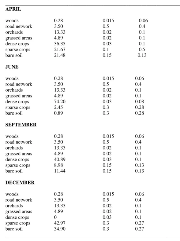
Transports, 2002; Rapport final de la Convention ADALI, 2002). Unfortunately, croplands 11
were only characterized by a global runoff coefficient and velocity in these studies. In order to 12
study the temporal variability of these parameters for croplands, the field survey method 13
developed by Cerdan et al. (2002) for the STREAM model was combined with the 14
experimental data for other types of land use from the studies mentioned above. The 15
STREAM model takes surface crusting, soil roughness and vegetation cover into account to 16
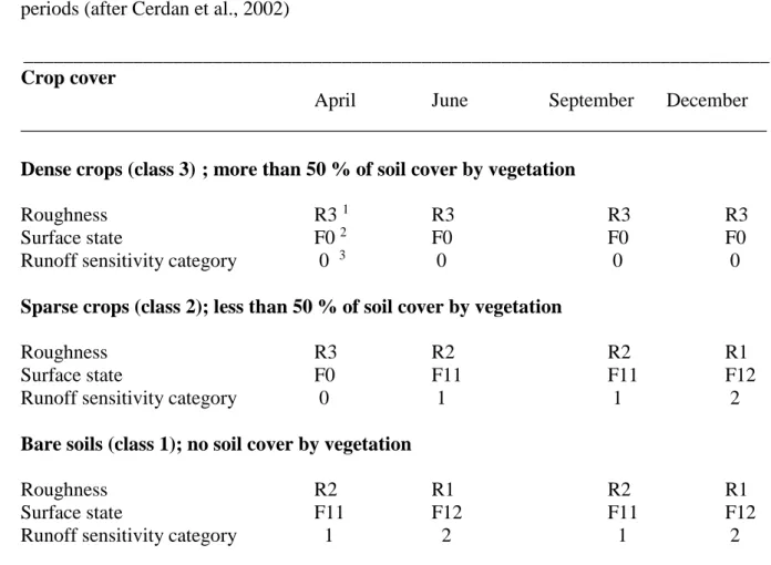
determine a relative category of runoff sensitivity. These categories were determined by field 17
surveys (Table 1). Runoff coefficients and velocities were then attributed to these relative 18
categories, in such a way that cropland values fall within the range of values for the other 19
types of land use from previous experimental studies carried out in the Belgian loam belt 20
(Table 2). The following sequence of increasing probability to generate runoff was used (e.g. 21
Musy and Higy, 2004): 22
Woodlands < Grassland < Dense crops < Sparse crops < Bare soils < Roads 23
24
2.5. Simulations 25
In order to select a worst-case scenario, four seasons are simulated, to evaluate the most 1
sensitive period for flooding. The land cover spatial datasets for each season are transformed 2
into two-meter gridcells. The model is run with the same rainfall event for the four different 3
land cover datasets. Furthermore, the impact of the land consolidation of 1977 is investigated 4
for this specific catchment. The former field pattern is mapped from digitised aerial 5
photographs of 1957. A visual observation of the photographs allowed the recognition of most 6
types of cover within the catchment. For the remaining 7% of the fields, the land cover from 7
agricultural statistics for the loam belt were used (Institut National de Statistiques, 1957). A 8
land cover class was randomly assigned to each field for which the cover was impossible to 9
distinguish on the photograph, according to these statistics. The impact of the GWW installed 10
in the thalweg in 2002 is analysed. For this purpose, the worst-case scenario is simulated. 11
Finally, the effect of the retention dam is also addressed. 12
13
2.6 Strengthening confidence in the model for extreme events 14
15
A validation of the MHM model has already been successfully implemented in catchments 16
under temperate and semi-arid climates (El Idrissi, 1996; Ntaguzwa, 1999; Hang, 2002). The 17
model is also used by the hydrological service (SETHY, Service d’ETudes HYdrologiques) of 18
the Walloon Region of Belgium. As the model does not simulate water reinfiltration, the 19
topographic index (eq. 3) has been computed at both extremities of the GWW to check its 20
topographic sensitivity to surface saturation (Beven and Kirkby, 1979; Moore et al., 1988). 21 tan ln I (3) 22
where I is the topographic index; α is the local catchment area per unit contour length and is 23
expressed in meters ;β is the slope of the ground surface (in degrees). Typically, a large local 24
catchment area and a small slope result in a high value of the index, meaning that the 25
groundwater table is located at a low depth and that wetter soil can be expected (Rodhe and 1
Seibert, 1999). 2
3
Furthermore, to increase the confidence in the model for this specific application, several 4
events were used for comparison of simulated discharges with the observed ones at the 5
catchment outlet. Water level measurements behind a dam are used. Water is temporally 6
stored in a retention pond and drains through two pipes of 0.25m and 0.2m diameter in the 7
bottom of the dam. Few runoff events have been recorded since 2003. A crest stage recorder 8
was installed behind the dam to measure water level when runoff to the outlet occurred. Such 9
a recorder consists of a plastic tube with a length of water-sensitive tape which changes 10
colour on contact with water (Hooke and Mant, 2000). Water levels were then converted to 11
outflow discharge of the pipes in the dam by eq. 4 (Ilaco, 1985). 12 h g A m Q 2 (4) 13
where Q is the discharge (m³.s-1); m is the discharge coefficient (here equal to 0.62); A is the 14
cross-section of the drain (m²); g is the gravity acceleration (9.81 m². s-1) and h is the 15
hydraulic head (m).A tipping bucket raingauge was installed 500 meters north of the outlet. 16
17
3. Results and discussion 18
19
3.1. Strenghtening confidence in the model 20
21
According to the litterature, we obtained very high values of the topographic index at the 22
GWW upstream extremity (I =16.1) and the catchment outlet (I =16.7). By comparison, 23
Beven and Wood (1983) found that the first saturated areas of a catchment had a topographic 24
index value close to 15. Rodhe and Steibert (1999) found maximal I values of ~17 in Swedish 25
catchments. This means that the GWW will be very quickly saturated during a storm. 26
Reinfiltration is hence highly unlikely in that place, and the hypothesis of the model is hence 1
acceptable. 2
3
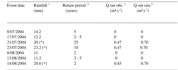
Runoff occurred three times in 2004 (Table 3). The occurrence of runoff is correctly predicted 4
even if the peak discharge is overestimated by ~50%. It remains hence in the same order of 5
magnitude. Other recorded rainfall events that did not lead to runoff at the outlet were 6
simulated with the model. Simulated runoff during these events was very low and completely 7
buffered by the retention dam. 8
9
3.2. Selection of a worst-case scenario 10
11
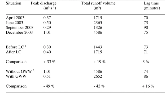
The simulation of the event with a 10 year return period shows that highest peak discharges 12
and runoff volumes are reached in December (1.0 m³.s-1; 4586 m³), while they are lowest in 13
September (0.3 m³.s-1; 1715 m³; Fig. 3; Table 4). These results are explained by the higher 14
proportion of bare soil (35 %) and sparsely covered soil (43 %) at the beginning of winter 15
(Fig. 2d). The December situation is hence chosen as a worst-case scenario. June is the second 16
highest risk period, because crop cover is quite low and crusts develop on these sparsely 17
covered soils (Fig.2b; Table 1). 18
19
3.3. Potential effect of land consolidation on runoff 20
21
After the 1977 consolidation, the mean size of the fields in the study area increased about 22
four-fold from 1.02 ha in 1957 to 4.34 ha in 2003. This is in agreement with Verstraeten and 23
Poesen (1999) and Beuselinck et al. (2000) who studied land consolidation in an area of 24
central Belgium. The land cover before the consolidation in the 1970s (Fig. 4a) is compared 25
to that of April 2003 (Fig. 4b). For an event with a 10 year return period, runoff volume 26
increased by 19 per cent following the land consolidation operation (from 1443 m³ in 1957 to 27
1715 m³ in 2003), while peak discharge rose by 33 per cent (Fig. 5), reaching 0.3 m³.s-1 for 1
the 1957 simulation, against 0.4 m³.s-1 in April 2003. The lag time is similar in both situations 2
and is close to 75 minutes (Fig. 5). However, the hydrograph shape is different. The rising 3
limb is more gradual before the land consolidation scheme. After land consolidation, the first 4
peak in the hydrograph, corresponds to the sudden arrival of water that concentrates on the 5
road in the thalweg. 6
7
In comparison with other studies, land consolidation does not lead to a sharp rise of runoff 8
volume (e.g. more than 75 % rise according to Souchère et al., 2003). Two reasons can be put 9
forward. First, the Belgian openfield context is different from that of bocage landscapes. In 10
the study area, no grassland or hedgerows were present before 1977. Consequently, there was 11
no ploughing up of grassed areas, which resulted in an important increase of runoff volume in 12
other European regions. Second, the model does not take into account the ditch network of the 13
catchment, where water can be temporally buffered. This impact is hence underestimated in 14
this study, which highlights the major role played by a consolidation road constructed in the 15
thalweg and leading to an increase of the runoff transfer velocity to the outlet (10 minutes-16
long sharp rising limb in 2003 instead of a more gradual rising limb lasting for 30 minutes in 17
1977). 18
3.4. Impact of the mitigation measures 19
20
The impact of the GWW (12 ha) installed in 2002 is simulated for the worst-case scenario 21
(Fig. 6). Peak discharge is reduced by 50 % when the GWW is taken into account (0.5 m³.s-1 22
instead of 1.0 m³.s-1 ; Fig. 7; Table 4). Runoff volume transferred to the outlet decreased by 40 23
per cent (2651 m³ instead of 4586 m³; Table 4). Another very interesting effect of GWW is 24
the lag time increase (+ 16%; Table 4). The rising limb is also more gradual when the GWW 25
is considered (Fig. 7). Results are difficult to compare with the ones obtained in other studies, 1
given the much smaller size of the studied catchments (15 ha in Fiener and Auerswald, 2003) 2
or a too different landscape context (GWW and terraces in the USA e.g. Chow et al., 1999). 3
However, these studies observe the same trends (decrease of both peak discharge and total 4
runoff volume). 5
6
The decrease in total runoff volume (1935 m³) when the GWW is considered can be explained 7
by two reasons. First, less runoff has been produced in the GWW due to its lower runoff 8
coefficient (680 m³). Second, a reduction in runoff velocity (0.1 m.s-1 instead of 0.27m.s-1) 9
upon replacing sparsely covered cropland with a GWW has resulted in a long-tail of runoff. 10
Remaining runoff volume at the outlet (1255 m³) is spread over a longer period. The model 11
does not simulate the whole recession limb in this case, given it is limited to a 180-minutes 12
simulation. 13
14
In relation to the flood risk in Velm village, the maximal observed outflow peak discharge 15
reached 0.47 m³.s-1 in 2004, which is very close to the one simulated by the model taking the 16
GWW into account (0.50 m².s-1; Table 4). No flooding of the village resulted in 2004. Given 17
the model overestimates the discharge by ~50% (Table 3), any new flooding of Velm is 18
highly unlikely for the selected worst-case scenario. As the retention pond buffers all the 19
incoming runoff, the diameter of the outflow pipes could be narrowed (with metal plates e.g.) 20
to limit runoff discharge towards the village. 21
22
4. Conclusions 23
This case study in a small agricultural catchment (c. 300 ha) of central Belgium shows that a 24
GWW and a retention dam alleviate the muddy floods risk for Velm village. Peak discharge 25
increases by 16%. However, land consolidation carried out in the 1970s led to an increase of 1
peak discharge (33%) and total runoff volume (19%). It is explained by a rise in field sizes 2
(from 1.02 ha in 1977 to 4.34 ha in 2003) but also and mainly by the construction of a road in 3
the thalweg of the catchment leading to runoff concentration. Consequently, on-site soil 4
conservation measures are to be installed within the catchment to prevent runoff generation 5
and mitigate its concentration in the catchment thalweg. Furthermore, as generated runoff 6
volume is buffered in the retention pond for the selected worst-case scenario, a reduction of 7
the outflow pipes diameter could be envisaged in order to limit the discharge towards the 8 village. 9 10 Acknowledgements 11 12
We are grateful to Matthieu Kervyn for his helpful comments on an earlier draft of this paper. 13 14 15 16 17 18 19 20 21 22 23 24 25 26 27 28 29 30 31 32 33 34 35 36 37 38 39
References 1
2
Ilaco, 1985. Agricultural Compendium for rural development. Elsevier, Amsterdam, 738 p. 3
4
Baeyens, L., 1958. Carte des sols de la Belgique. Texte explicatif de la planchette de Sint-5
Truiden 105 E. (In Dutch and French). Institut pour l’encouragement de la Recherche 6
Scientifique dans l’Industrie et l’Agriculture, Brussels. 7
8
Beuselinck, L., Steegen, A., Govers, G., Nachtergaele, J., Takken, I., Poesen, J., 2000. 9
Characteristic of sediment deposits formed by intense rainfall events in small catchments in 10
the Belgian Loam Belt. Geomorphology 32, 69 – 82. 11
12
Beven, K.J., Kirkby, M.J., 1979. A physically based, variable contributing area model of 13
basin hydrology. Hydrolog. Sci. – Bulletin des Sciences Hydrologiques 24, 43-69. 14
15
Bielders, C.L., Ramelot, C., Persoons, E., 2003. Farmer perception of runoff and erosion and 16
extent of flooding in the silt-loam belt of the Belgian Walloon Region. Environmental Science 17
and Policy 6, 85 – 93. 18
19
Boardman, J., Ligneau, L., De Roo, A., Vandaele, K., 1994. Flooding of property by runoff 20
from agricultural land in northwestern Europe. Geomorphology 10, 183-196. 21
22
Boardman, J., Evans, R., Ford, J., 2003. Muddy floods on the South downs, southern 23
England: problem and responses. Environmental Science and Policy 6, 69-83. 24
25
Cerdan, O., Couturier, A., Le Bissonnais, Y., Lecomte, V., Souchère, V., 2001. Incorporating 1
soil surface crusting processes in an expert-based runoff model: Sealing and Transfer by 2
Runoff and Erosion related to Agricultural Management. Catena 46, 189-205. 3
4
Cerdan, O., Le Bissonnais, Y., Souchère, V., Martin, P., Lecomte, V., 2002. Sediment 5
concentration in interrill flow : Interactions between soil surface conditions, vegetation and 6
rainfall. Earth Surf. Process. Landforms 27, 193-205. 7
8
Chaplot, V., Le Bissonnais, Y., 2000. Field measurements of interrill erosion under different 9
slopes and plot sizes. Earth Surf. Process. Landforms 25, 145-153. 10
11
Chow,T.L., Rees, H.W., Daigle, J.L., 1999. Effectiveness of terraces/grassed waterway 12
systems for soil and water conservation: A field evaluation. J. Soil Water Conserv. 3, 577-13
583. 14
15
Delbeke, L., 2001. Extreme neerslag in Vlaanderen. (In Dutch). AMINAL, Afdeling Water. 16
Ministerie van de Vlaamse Gemeenschap. 17
18
El Idrissi, A., 1996. Effet de l’humidité initiale du sol sur le processus de ruissellement à 19
l’échelle de la parcelle et du bassin versant. (In French). Unpublished PhD thesis. Agricultural 20
Engineering Unit, Université Catholique de Louvain. 21
22
El Idrissi, A., Persoons, E., 1997. MHM : le Modèle Hydrologique Maillé.(In French). In : 23
FAO : “Remote Sensing and Water Resources”. Proceedings of the international workshop, 24
Montpellier (France). 25
World Wide Web Address : 1
http://www.fao.org/documents/show_cdr.asp?url_file=/docrep/W7320B/w7320b37.htm
2 3
Fiener, P., Auerswald, K., 2003. Concepts and effects of a multi-purpose grassed waterway. 4
Soil Use and Management 19, 65 – 72. 5
Fiener, P., Auerswald, K., 2005. Seasonal variation of grassed waterway effectiveness in 6
reducing runoff and sediment delivery from agricultural watersheds in temperate Europe. Soil 7
and Tillage Research, in press. 8
9
Hang, P., 2002. Conception et développement du modèle OGIVE et application à des micro-10
bassins versants belges. (In French). Unpublished PhD thesis, Faculty of Biological, 11
Agronomical and Environmental Engineering, Université Catholique de Louvain. 12
13
Hooke, J.M., Mant, J.M., 2000. Geomorphological impacts of a flood event on ephemeral 14
channels in SE Spain. Geomorphology 34, 163-180. 15
16
Hufty, A., 2001. Introduction à la climatologie. (In French). Ed. De Boeck Université, 17
Brussels, 542 p. 18
19
Institut National de Statistiques, 1957. Recensement agricole et horticole au 15 mai 1957. (In 20
French). Brussels, Ministère des Affaires économiques. 21
22
Le Bissonnais, Y., Lecomte, V., Cerdan, O., 2004. Grass strip effects on runoff and soil loss. 23
Agronomie 24, 129-136. 24
Linsley, R.K., Franzini, J.B., Freyberg, D.L., Tchobanoglous, G., 1992. Water Resources 1
Engineering. 4th edition. Ed. Mac Graw-Hill, 841 p. 2
3
Ministère de l’Equipement et des Transports. Direction des Routes de Liège, 2002. Bilan de 4
fonctionnement hydraulique et écologique des bassins d’orage de l’autoroute E40. Rapport 5
final. (In French). Groupe Interuniversitaire de Recherches en Ecologie Appliquée (GIREA) 6
and Agricultural Engineering Unit, Faculty of Biological, Agronomical and Environmental 7
Engineering, Université Catholique de Louvain. 8
9
Moore, I.D., Burch, G.J., Mackenzie, D.H., 1988. Topographic effects on the distribution of 10
surface soil water and the location of ephemeral gullies. Transactions of the ASAE 31(4), 11
1098-1107. 12
13
Musy, A., Higy, C., 2004. Hydrologie. Une science de la nature. (In French). Presses 14
Polytechniques et Universitaires Romandes, Lausanne, 314 p. 15
16
Ntaguzwa, D., 1999. La relation pluie-débit et l’incertitude en modélisation hydrologique. 17
Application aux bassins versants du complexe des barrages de l’Eau d’Heure (Belgique). (In 18
French). Unpublished PhD thesis. Agricultural Engineering Unit, Université Catholique de 19
Louvain. 20
21
Randriamaherisoa, A., 1993. Modèle Hydrologique Maillé et Système d’Information 22
Géographique. L’impact de la déforestation sur le régime hydrologique de la Lokoho 23
(Madagascar). (In French). Unpublished PhD thesis. Agricultural Engineering Unit, 24
Université Catholique de Louvain. 25
1
Rapport final de la Convention ADALI (Adaptation des Aménagements hydrauliques à la 2
Lutte contre les Inondations), 2002. (In French). Agricultural Engineering Unit, Faculty of 3
Biological, Agronomical and Environmental Engineering, Université Catholique de Louvain. 4
5
Rodhe, A., Seibert, J., 1999. Wetland occurrence in relation to topography: a test of 6
topographic indices as moisture indicators. Agricultural and Forest Meteorology 98-99, 325-7
340. 8
Souchère, V., King, C., Dubreuil, N., Lecomte-Morel, V., Le Bissonnais, Y., Chalat, M., 9
2003. Grassland and crop trends: role of the European Union Common Agricultural Policy 10
and consequences for runoff and soil erosion. Environmental Science and Policy 6, 7 – 16. 11
12
Steegen, A., Govers, G., Nachtergaele, J., Takken, I., Beuselinck, L., Poesen, J., 2000. 13
Sediment export by water from an agricultural catchment in the Loam Belt of central 14
Belgium. Geomorphology 33, 25-36. 15
16
Vandaele, K., Poesen, J., 1995. Spatial and temporal patterns of soil erosion rates in an 17
agricultural catchment, central Belgium. Catena 25, 213 – 226. 18
19
Verstraeten, G., Poesen, J, 1999. The nature of small-scale flooding, muddy floods and 20
retention pond sedimentation in central Belgium. Geomorphology 29, 275-292. 21
22
Verstraeten, G., Poesen, J., Govers, G., Gillijns, K., Van Rompaey, A., Van Oost, K., 2003. 23
Integrating science, policy and farmers to reduce soil loss and sediment delivery in Flanders, 24
Belgium. Environmental Science and Policy 6, 95 – 103. 25
Tables
12
Table 1. Runoff sensitivity relative categories for the different crop cover classes and survey 3
periods (after Cerdan et al., 2002) 4 5 ___________________________________________________________________________ 6 Crop cover 7
April June September December
8
___________________________________________________________________________ 9
10
Dense crops (class 3) ; more than 50 % of soil cover by vegetation 11 12 Roughness R3 1 R3 R3 R3 13 Surface state F0 2 F0 F0 F0 14
Runoff sensitivity category 0 3 0 0 0
15 16
Sparse crops (class 2); less than 50 % of soil cover by vegetation 17 18 Roughness R3 R2 R2 R1 19 Surface state F0 F11 F11 F12 20
Runoff sensitivity category 0 1 1 2
21 22
Bare soils (class 1); no soil cover by vegetation 23 24 Roughness R2 R1 R2 R1 25 Surface state F11 F12 F11 F12 26
Runoff sensitivity category 1 2 1 2
27
___________________________________________________________________________ 28
29
1 R : soil surface roughness state (height difference between the deepest part of 30
microdepressions and the lowest point of their divide). R0 : 0-1 cm; R1 : 1-2 cm; R2 : 2-5 cm; 31
R3 : 5-10 cm. 32
33
2 F: soil surface crusting stage. F0 : initial fragmentary structure; F11 : altered fragmentary 34
state with structural crusts; F12 : local appearance of depositional crusts; F2 : continuous 35
crusts. 36
37
3 :The runoff sensitivity category range from 0 to 2. The greater the value of the category, the 38
greatest potential to generate runoff. 39 40 41 42 43 44 45 46 47 48 49
Table 2. Runoff coefficients and velocities for different months and different land cover 1
classes in the study area 2
3
__________________________________________________________________ 4
5
Land cover Study area covered (%) Runoff coefficient Runoff velocity (m/s) 6 ________________________________________________________________________ 7 APRIL 8 9 woods 0.28 0.015 0.06 10 road network 3.50 0.5 0.4 11 orchards 13.33 0.02 0.1 12 grassed areas 4.89 0.02 0.1 13 dense crops 36.35 0.03 0.1 14 sparse crops 21.67 0.1 0.5 15 bare soil 21.48 0.15 0.13 16 17 JUNE 18 19 woods 0.28 0.015 0.06 20 road network 3.50 0.5 0.4 21 orchards 13.33 0.02 0.1 22 grassed areas 4.89 0.02 0.1 23 dense crops 74.20 0.03 0.08 24 sparse crops 2.45 0.3 0.28 25 bare soil 0.89 0.3 0.28 26 27 SEPTEMBER 28 29 woods 0.28 0.015 0.06 30 road network 3.50 0.5 0.4 31 orchards 13.33 0.02 0.1 32 grassed areas 4.89 0.02 0.1 33 dense crops 40.89 0.03 0.1 34 sparse crops 8.98 0.15 0.13 35 bare soil 11.44 0.15 0.13 36 37 DECEMBER 38 39 woods 0.28 0.015 0.06 40 road network 3.50 0.5 0.4 41 orchards 13.33 0.02 0.1 42 grassed areas 4.89 0.02 0.1 43 dense crops 0 0.03 0.1 44 sparse crops 42.97 0.3 0.27 45 bare soil 34.90 0.3 0.27 46 _________________________________________________________________ 47 48 49 50 51 52 53
Table 3. Rainfall and discharge in 2003 and 2004 1
__________________________________________________________________________________ 2
Event date Rainfall 1 Return period 2 Q out obs. 3 Q out sim.4
3 (mm) (years) (m³.s-1) (m³.s-1) 4 5 __________________________________________________________________________________ 6 7 8/07/2004 14.2 5 0 0 8 17/07/2004 12.2 2 - 5 0 0 9 21/07/2004 20 (*) 25 0.47 0.70 10 23/07/2004 23.2 (*) 10 0.47 0.70 11 8/08/2004 11 2 0 0 12 13/08/2004 11.2 2 - 5 0 0 13 14/08/2004 20.6 (*) 2 0.45 0.70 14 __________________________________________________________________________________ 15 16
1Discharge at the outlet was recorded for the events with (*).
17
2 Return periods after Delbeke (2001). They are computed for the rainfall duration considered.
18
3 Q out obs. is the outflow discharge calculated from H obs. with eq. (3).
19
4 Q out sim. is the simulated outflow discharge after introduction in the MHM model.
20 21 22 23 24 25 26 27 28 29 30 31 32 33 34 35 36 37 38 39 40 41 42 43 44 45 46 47 48 49
Table 4. Peak discharge, total runoff volume and lag time at the catchment outlet for the 1
different situations simulated with the MHM model 2
___________________________________________________________________________ 3
Situation Peak discharge Total runoff volume Lag time
4 (m³.s-1) (m³) (minutes) 5 ___________________________________________________________________________ 6 April 2003 0.37 1715 70 7 June 2003 0.50 2365 73 8 September 2003 0.29 1326 90 9 December 2003 1.01 4586 75 10 11 12 Before LC 1 0.30 1443 73 13 After LC 0.40 1715 71 14 15 Comparison + 33 % + 19 % - 3 % 16 17 Without GWW 2 1.01 4586 74 18 With GWW 0.51 2652 86 19 20 Comparison - 49 % - 42 % + 16 % 21 ___________________________________________________________________________ 22 23
1 LC : land consolidation (April situation) 24 2 GWW: grassed waterway 25 26 27 28 29 30 31 32 33 34 35 36 37 38 39 40 41 42 43 44 45 46 47 48
Captions of figures
1 2
Figure 1. Location map of Velm village, the upstream agricultural catchments and land use of 3
the study area. 4
5
Figure 2. Seasonal evolution of land cover in the study area 6
(a) April; (b) June; (c) September; (d) December 7
8
Figure 3. Discharge at the catchment outlet in different seasons according to land cover in 9
2003 (see the corresponding land cover maps on Fig. 2) 10
11
Figure 4. Land use and land cover before (a) and after (b) land consolidation 12
13
Figure 5. Simulated hydrographs at the catchment outlet for the situation before and after 14
the land consolidation 15
16
Figure 6. Grassed waterway and other land covers in December 2003 17
18
Figure 7. Hydrograph at the catchment outlet for the December situation, with and without 19 grassed waterway 20 21 22 23
Outlet
¯
0 250 500 1.000 Meters Land cover Woodland Roads Orchards Grassland Cropland (a) (b)¯
Legend Limits of catchment Molenbeek river Village Study area 0 750 1.500 3.000 Meters Gingelom village Velm villageOutlet Outlet (a) (b) Outlet Land cover Permanent cover Dense crops Sparse crops Bare soils Outlet
¯
0 250 500 1.000 Meters (c) (d) Figure 20 20 40 60 80 100 120 140 0 10 20 30 40 50 60 70 80 90 100 110 120 130 140 150 160 170 180 Time (minutes) R a in fa ll i n te n s it y ( m m /h ) 0.0 0.2 0.4 0.6 0.8 1.0 1.2 D is c h a rg e a t th e o u tl e t (m ³/ s )
Rainfall Discharge (April) Discharge (June)
Discharge (Sept) Discharge (Dec)
Outlet Land cover Permanent cover Dense crops Sparse crops Bare soils Outlet
¯
0 250 500 1.000 Meters (a) (b) Figure 40 20 40 60 80 100 120 140 0 10 20 30 40 50 60 70 80 90 100 110 120 130 140 150 160 170 180 Time(minutes) R a in fa ll i n te n s it y ( m m /h ) 0.00 0.05 0.10 0.15 0.20 0.25 0.30 0.35 0.40 D is c h a rg e a t th e o u tl e t (m ³/ s )
Rainfall Discharge before consolidation Discharge after consolidation
Outlet
¯
0 250 500 1.000 Meters Land cover Permanent cover Grassed waterway Sparse crops Bare soils Figure 60 20 40 60 80 100 120 140 0 10 20 30 40 50 60 70 80 90 100 110 120 130 140 150 160 170 180 Time (minutes) R a in fa ll i n te n s it y ( m m /h ) 0.0 0.2 0.4 0.6 0.8 1.0 1.2 D is c h a rg e a t th e o u tl e t( m ³/ s )
Rainfall Hydrogram without grassed waterway Hydrogram with grassed waterway