Climate of the last glacial maximum: sensitivity studies and model-data comparison with the LOVECLIM coupled model

(1)

HAL Id: hal-00298161

https://hal.archives-ouvertes.fr/hal-00298161

Submitted on 8 Nov 2006

HAL is a multi-disciplinary open access

archive for the deposit and dissemination of sci-entific research documents, whether they are pub-lished or not. The documents may come from teaching and research institutions in France or abroad, or from public or private research centers.

L’archive ouverte pluridisciplinaire HAL, est destinée au dépôt et à la diffusion de documents scientifiques de niveau recherche, publiés ou non, émanant des établissements d’enseignement et de recherche français ou étrangers, des laboratoires publics ou privés.

Climate of the last glacial maximum: sensitivity studies

and model-data comparison with the LOVECLIM

coupled model

D. M. Roche, T. M. Dokken, H. Goosse, H. Renssen, S. L. Weber

To cite this version:

D. M. Roche, T. M. Dokken, H. Goosse, H. Renssen, S. L. Weber. Climate of the last glacial maximum: sensitivity studies and model-data comparison with the LOVECLIM coupled model. Climate of the Past Discussions, European Geosciences Union (EGU), 2006, 2 (6), pp.1105-1153. �hal-00298161�

(2)

CPD

2, 1105–1153, 2006

The last glacial maximum climate and the LOVECLIM

model: a study D. M. Roche et al. Title Page Abstract Introduction Conclusions References Tables Figures J I J I Back Close Full Screen / Esc

Printer-friendly Version Interactive Discussion Clim. Past Discuss., 2, 1105–1153, 2006

www.clim-past-discuss.net/2/1105/2006/ © Author(s) 2006. This work is licensed under a Creative Commons License.

Climate of the Past Discussions

Climate of the Past Discussions is the access reviewed discussion forum of Climate of the Past

Climate of the last glacial maximum:

sensitivity studies and model-data

comparison with the LOVECLIM coupled

model

D. M. Roche1, T. M. Dokken2, H. Goosse3, H. Renssen1, and S. L. Weber4

1

Department of Palaeoclimatology and Geomorphology, Faculty of Earth and Life Sciences, Vrije Universiteit Amsterdam, De Boelelaan 1085, 1081 HV Amsterdam, The Netherlands

2

Bjerknes Center for Climate Research, Allegaten 55, 5007 Bergen, Norway

3

Institut d’Astronomie et de G ´eophysique G. Lemaˆıtre. 2, Chemin du Cyclotron, 1348 Louvain-la-Neuve, Belgium

4

Royal Netherlands Meteorological Institute (KNMI), P.O. Box 201, 3730 AE De Bilt, The Netherlands

Received: 9 October 2006 – Accepted: 3 November 2006 – Published: 8 November 2006 Correspondence to: D. M. Roche (didier.roche@falw.vu.nl)

(3)

CPD

2, 1105–1153, 2006

Printer-friendly Version Interactive Discussion

Abstract

The Last Glacial Maximum climate is one of the classic benchmarks used both to test the ability of coupled models to simulate climates different from that ot the present-day and to better understand the possible range of mechanisms that could be involved in future climate change. It also bears the advantage of being one of the most well

docu-5

mented periods with respect to palaeoclimatic records, allowing a thorough data-model comparison. We present here an ensemble of Last Glacial Maximum climate simula-tions obtained with the Earth System model LOVECLIM, including coupled dynamic atmosphere, ocean and vegetation components. The climate obtained using stan-dard parameter values is then compared to available proxy data for the surface ocean,

10

vegetation, oceanic circulation and atmospheric conditions. Interestingly, the oceanic circulation obtained resembles that of the present-day, but with increased overturn-ing rates. As this result is in contradiction with the “classic” palaeoceanographic view, we ran a range of sensitivity experiments to explore the response of the model and the possibilities for other oceanic circulation states. After a critical review of our LGM

15

state with respect to available proxy data, we conclude that the balance between water masses obtained is consistent with the available data although the specific characteris-tics (temperature, salinity) are not in full agreement. The consistency of the simulated state is further reinforced by the fact that the mean surface climate obtained is shown to be generally in agreement with the most recent reconstructions of vegetation and

20

sea surface temperatures, even at regional scales.

1 Introduction

In recent years, the Last Glacial Maximum (LGM) has become a standard period to benchmark the capability of climate models to simulate a drastically different cli-mate than that of the present-day. Several projects have reconstructed maps of the

25

(4)

CPD

2, 1105–1153, 2006

Printer-friendly Version Interactive Discussion GLAMAP2000 (Sarnthein et al., 2003) or MARGO (Kucera et al., 2005a), providing

strong constraints on what the climate looked like at that period of time. At the same time, efforts have been undertaken to better inter-compare the different models under glacial boundary conditions such as the pioneering work of the Palaeoclimate Modeling Intercomparison Project (PMIP) with Atmospheric General Circulation models (

Jous-5

saume and Taylor, 2000) and in its second phase with Coupled Atmospheric-Ocean models (Crucifix et al., 2005). Comparisons between PMIP models were also con-ducted to evaluate the results against surface data of the LGM (Kageyama et al.,2001,

2006). Those comparisons have shown that the inclusion of more components in the climate system have enabled the production of results which are in better agreement

10

with the data.

However, there is still strong disagreement between models with respect to one of the major components of the climate system: the oceanic thermohaline circulation (THC). In the few LGM experiments conducted with coupled Atmosphere–Ocean models (

Ki-toh et al.,2001; Hewitt et al., 2003;Shin et al.,2003; Kim,2004) the strength of the

15

thermohaline circulation and the relative importance of the different water masses dif-fers considerably. Mechanisms underlying the simulated THC response were found to differ widely in an inter-comparison study of PMIP coupled model simulations (Weber

et al.,2006). The “classic” palaeoceanographic interpretation of the data is a weaker overturning, with a less deep north Atlantic water mass and a denser and more

pre-20

dominant Antarctic water mass. However, some uncertainties remain on the precise relationships between the water masses.

In this study, we perform a suite of sensitivity studies of the response of the glacial ocean circulation to different parameters of the model. The aim is to assess how dif-ferent set-ups may yield different types of global meridional circulation. We will also

25

extensively compare our surface simulated LGM climate with available data (in partic-ular with the recently released MARGO database) to evaluate the agreement between the two. In particular we address whether a simulated oceanic circulation in contradic-tion with the one evaluated from the data causes a major mismatch in the simulated

(5)

CPD

2, 1105–1153, 2006

Printer-friendly Version Interactive Discussion surface climate, or whether, given the data currently available, agreement is still

ob-tained between surface data and model.

A precise definition of the LGM is required. Although it originally refers to the max-imum of globally averaged continental ice that occurred during the last glacial period, it is usually difficult to derive that period from a given data archive. Thus, the period

5

taken depends on the archive (Sarnthein et al.,2003, for example). In this paper, we will further refer to the LGM as the period around 21 thousand years before present (kyrs B.P.), coherent with the commonly used time period in previous climate simu-lations and being also the centre of the period used in most recent reconstructions (Kucera et al.,2005a).

10

2 The LOVECLIM model and the LGM

2.1 Model description

In this study we use the three-dimensional Earth System model LOVECLIM. LOVE-CLIM is an acronym made from the names of the five different models that have been coupled to build the Earth system model: LOch-Vecode–Ecbilt–CLio–agIsm

15

Model (LOVECLIM,Driesschaert,2005). Here only the atmosphere–ocean–vegetation part is used (ECBilt–CLIO–VECODE). Actually, in the configuration chosen here, the model gives exactly the same results as ECBilt-CLIO-VECODE version 3, used for instance by Goosse et al. (2005) and Renssen et al. (2005) to study the climate of the past millennium and of the Holocene respectively (but is substantially different

20

from the one used by Timmermann and Goosse,2004)). Nevertheless, many tech-nical changes have been included in the code recently, in particular in order to al-low for the coupling with ice sheet and carbon cycle models. As a consequence, for simplicity, users and developers have decided jointly that the new name LOVECLIM should now be used for the model, even if some components are not activated (see

25

(6)

CPD

2, 1105–1153, 2006

Printer-friendly Version Interactive Discussion The atmospheric model is a global quasi-geostrophic, spectral model at T21

hori-zontal resolution, with additional parameterisations for the diabatic heating due to ra-diative fluxes, the release of latent heat, and the exchange of sensible heat with the surface (Opsteegh et al.,1998). The ocean part is a three dimensional, free surface, general circulation model coupled to a thermodynamical and dynamical sea-ice model

5

(Goosse and Fichefet,1999). The vegetation part is the VECODE dynamical terrestrial vegetation model (Brovkin et al.,1997) which computes plant fractions for trees and herbaceous (plus desert) from several atmospheric variables in each land grid-cell. To easily compare the output of VECODE with available vegetation reconstructions for the LGM, we developed a module to assign biomes from the Plan Functional Types (PFTs)

10

computed by the vegetation model (see2.3).

As such, the Earth system model used here is able to simulate the climate with some details while still being computationally efficient, and therefore allows for multi-millenial simulations. This ability is used extensively here, in order to test the model with respect to the different parameter values in the range of possibilities, in particular with respect

15

to the oceanic circulation.

This coupled model was validated for the pre-industrial climate (Driesschaert,2005), a state used here as starting point for our simulations. It will be hereafter referred to as LH CTRL (Late Holocene, used as Control).

2.2 LGM boundary conditions

20

To simulate the Last Glacial Maximum (LGM) climate, we use the following bound-ary conditions. Atmospheric greenhouse gases concentrations are modified (Fluckiger

et al.,1999;D ¨allenbach et al.,2000;Monnin et al.,2001), that is forcing for CO₂(also taken into account in the vegetation partHarrison and Prentice,2003), CH₄ and NO₂ trace gases (with values of 185 p.p.m., 350 p.p.b. and 200 p.p.b. respectively).

Modifi-25

cation of the insolation parameters is set as for 21 kyrs B.P. (Berger and Loutre,1992). The additional dust forcing due to the ice-age atmospheric dust loading (Claquin et al.,

2003) is taken into account in the incoming solar radiation at the top of the atmosphere. 1109

(7)

CPD

2, 1105–1153, 2006

Printer-friendly Version Interactive Discussion Ice-sheet topography changes are taken fromPeltier(2004) and the surface albedo is

set accordingly. The land-sea mask and the oceanic bathymetry are modified to ac-count for the lowered sea-level by 120 m relative to present (Lambeck and Chappell,

2001). Also included are changes in the river basins, i.e. changes in river routing due to the presence of ice-sheets. This mainly concerns the northern hemisphere; north

5

America with changes in the output of water from the Laurentide ice-sheet and Eurasia with changes over the Fennoscandian ice-sheet. We include changes in “river runoff” occurring from Antarctica (i.e. calving) which is displaced towards the equator, to ac-count for the likely location of melting of icebergs in this colder climate, as is shown by iceberg models (J. Jongma, personal communication).

10

We then applied these forcings to the model taken in the LH CTRL state and inte-grated it until equilibrium, reached after about 5000 years of integration.

2.3 Biome estimations from VECODE

To better compare the results of VECODE (Brovkin et al.,1997) with proxy data, we have developed a module to compute biomes, using both VECODE and ECBilt output.

15

This module is based on the approach of Prentice et al. (1992), with some simplifi-cations. We here considered only the 12 biomes thought to be the most appropriate with respect to the level of the complexity of the VECODE vegetation model and the resolution of the ECBilt atmospheric model. In particular, VECODE only computes two main Plant Functional Types (PFTs): herbaceous and trees. The “tree” PFT is split in

20

terms of needleleaved and broadleaved trees. It also computes a desert fraction. The sum of the three fractions (trees, herbaceous and desert) equals one. In cells with a prescribed ice-sheet, we assign all PFTs’ fractions to zero and the desert fraction to 1. The environmental limits used to convert the PFT distribution computed by VECODE are given in Table1. For each cell, we first compute the dominating PFT in the cell and

25

then apply the environmental constraints in order to assign a biome. In contrast with

Prentice et al.(1992), we did not retain any biomes based on the dominance of shrubs as they are not a PFT in VECODE.

(8)

CPD

2, 1105–1153, 2006

Printer-friendly Version Interactive Discussion Additionally, we have added a tree growing limitation with respect to CO₂in order to

take into account the effect of higher herbaceous competitiveness under lowered at-mospheric CO₂conditions (Harrison and Prentice,2003), as has been the case during the LGM.

3 Overview of the simulated LGM climate

5

3.1 Surface Air Temperature (SAT) changes

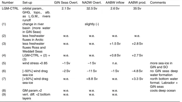
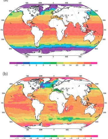
The simulated LGM climate we obtain presents a reduction of –4.4◦C in global mean surface temperature. This result compares well with the PMIP2 models’ mean changes of –4.45◦C (Kageyama et al.,2006, for 6 models) in air temperature. Figure 1 presents the change in global surface temperature between LGM and LH CTRL, together with

10

the changes in seasonality amplitude simulated under LGM conditions with respect to LH CTRL.

Changes in SAT (Fig.1a) show much colder temperatures on the prescribed perma-nent ice-sheet (up to –30◦C in the centre of Laurentide and Fennoscandian ice-sheets , and up to –6◦C at the border) due to the changes of altitude and albedo. Differences

15

of –6 to –15◦C are simulated over the additional sea-ice covered regions as a response to seasonal or perennial isolation from the atmosphere and albedo effect. Nearby land points also exhibit comparable changes due to the albedo effect of increased snow cover. A cooling of 1 to 2◦C is simulated in most of the tropical and equatorial regions with the exception of no changes over the north of Australia (Sea of Arafora).

20

We define the seasonal range as being the warmest–coldest month anomaly in sur-face air temperature. LGM to LH CTRL differences in seasonal range are shown in Fig.1b. The seasonal range at the LGM is increased globally by 9.7◦C with respect to the LH CTRL simulation. This number however hides large regional differences. We can distinguish three different zones. a) LGM ice-sheet regions like North America and

25

Scandinavia where the seasonal range is much less than in the LH CTRL simulation 1111

(9)

CPD

2, 1105–1153, 2006

Printer-friendly Version Interactive Discussion (–4 to –20◦C). This is due to the fact that these regions have a high seasonal range in

the present-day, but the seasonal differences are dampened by the all-year cold climate of the LGM, due to the presence of the ice-sheets (this also holds for the Patagonian ice-cap). This is also true for nearby regions like Siberia, where the seasonal range is reduced due to longer snow cover and cooler summers. b) regions where there are

al-5

ready ice-sheets in the present-day (Greenland, Antarctica) and over oceans between 40◦N and 40◦S. These regions undergo small SAT seasonality changes with respect to the LH CTRL (–1 to 1◦C), as they are much unchanged by the LGM climate (mainly cooled down by a few degrees). c) over continental regions in general (and extended deserts in particular), oceans near to ice-sheets and extended sea-ice cover regions

10

which have a much higher seasonality in the LGM than in the present-day. All these regions are much colder at the LGM during winter time (extension of sea-ice enhanced the effect, neighboring ice-sheet implying snow cover, colder inland and bright desert regions – all an albedo effect, mainly).

3.2 Changes in the hydrological cycle

15

In the global mean, there is a decrease of the total amount of precipitation by 13 mm.yr-1, consistent with a decrease in the evaporation due to the global cooling (see Fig.2a). Some regions undergo a drastic reduction in the rate of annual mean precipitation, such as the southern border of the Sahara, the middle- and far- East, some parts of central Asia (in particular the Tibetan Plateau) and central Greenland –

20

a feature consistent with snow accumulation data (Cuffey and Clow,1997;Alley,2000) – and Western Canada. There is also some consequent diminution of precipitation in southern Europe – consistent with both other model results and proxy data (Tarasov

et al.,1999;Peyron et al.,2005;Jost et al.,2005) –, some parts of Siberia, Svalbard, Japan and southern America (Argentina and southern Chile). The decrease of

pre-25

cipitation observed in south America is consistent with the fact that this region was a source of dust in the LGM (Grousset et al.,1992;Basile et al.,1997).

(10)

CPD

2, 1105–1153, 2006

Printer-friendly Version Interactive Discussion hemisphere are mainly due to the displacement of the winds tracks, as a consequence

of the presence of ice-sheets. Interestingly, the simulated changes show a maximum increase of precipitation over the southern border of the Laurentide ice-sheet (a feature also reported byKageyama and Valdes,2000 and Vettoretti et al.,2000) and on the western flank of the Fennoscandian ice-sheet. The increase in precipitation over these

5

areas is crucial for maintaining ice-sheets at the LGM, both for the southern part of the Laurentide ice-sheets, which presents a lobe advance in this region (Peltier,2004), and for the Fennoscandian ice-sheet. It is an important pre-requisite to be able to simulate the advance and volume of the last glacial ice-sheets, especially the Fennoscandian one (Forsstr ¨om and Greve,2004;Charbit et al.,2006).

10

The changes in the precipitation pattern in the LGM therefore seem to be quite com-parable with other LGM studies (Vettoretti et al.,2000) as well as favourable to maintain the extensive (prescribed here) ice-sheet of the LGM period.

3.3 Changes in simulated vegetation cover

Globally the simulated changes in vegetation cover are respond to the cooling and

dry-15

ing conditions which prevail in the simulated LGM climate described here. For the three Plant Functional Types (PFTs) simulated, VECODE simulates the following evolutions in the LGM with respect to LH CTRL.

The desert fraction is expanded in central Asia, the Sahara and southeast America, reflecting the drier conditions prevailing there. Some polar desert appears in

north-20

eastern Siberia (which denotes extreme cold and dry conditions, compatible with the absence of an ice-sheet in this area during the LGM, seeSvendsen et al.,2004).

Tree fractions are reduced overall, as low as zero in certain regions. For example, the cooling of the climate and the lowering of the atmospheric CO₂level causes disap-pearance of the LH CTRL forests of central Russia and Siberia in favour of herbaceous

25

areas. The model furthermore simulates the shrinking of the tropical broadleaf forests (Amazonia and tropical Africa) in response to the drying conditions (see Fig.2a). In the case of northern America, we can make a direct comparison between simulated

(11)

CPD

2, 1105–1153, 2006

Printer-friendly Version Interactive Discussion PFTs and data for the tree cover in the LGM (Williams,2002). VECODE correctly

sim-ulates a mixture of needleleaved and broadleaved trees on the east coast of America, with a high tree cover until the southern boundary of the Laurentide ice-sheet. The central part of the United States is correctly covered predominantly by grass with few trees (0–15%). However, our simulation shows dense tree cover in the western United

5

States for the LGM, a feature which is not seen in teh proxy data (Williams,2002). This feature is also present in the LH CTRL simulation which shows a too large tree cover in this region for the Late Holocene. This is due to the too humid state simulated in this area for both climates.

Grass fractions are increased in regions where the tree area shrinks, and in particular

10

in central Asia, southern Europe, western Africa and eastern Brazil.

All these changes are broadly consistent with the changes found in pollen distribu-tions for the LGM (Prentice et al., 2000, for example). However, as it is common to describe the reconstructions of vegetation in terms of biomes, we considered it useful to develop an approach that computes biomes from the available PFTs distribution and

15

climatic variables in a simple manner (as presented above). The results obtained in this development are described below, and enable a detailed data-model comparison for our simulated LGM climate.

3.4 Overview of the simulated deep ocean circulation

The location of deep water formation in the northern hemisphere is shifted from the

20

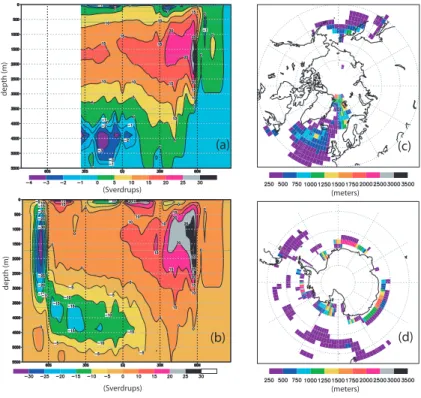
Labrador and Nordic seas for the LH CTRL run to the south of Iceland and Greenland in our LGM simulation, with some convection remaining in the Nordic seas (Fig.3c). These changes are accompanied by a reduction of the maximum depth of direct ven-tilation by about 600 m. The maximum convection depth is still reached in the Nordic seas (1800 m), marginally deeper than south of Iceland (1400 m). However, the

con-25

vection site south of Iceland is more permanent, whereas the activity of the Nordic Seas site depends on the year considered.

(12)

convec-CPD

2, 1105–1153, 2006

Printer-friendly Version Interactive Discussion tion, but an important shift in the location of deep water production (Fig.3d). Whereas

in LH CTRL sinking waters are formed partly along the coast of Antarctica (plus the Weddell and Ross seas) and partly further away from the continent, this latter source disappears in the LGM simulation and the former is reinforced. There is open ocean convection along the coast of Antarctica in all sectors of the Southern Ocean, the

5

strongest and deepest being in the Atlantic sector. As a result of this shift in the loca-tion of convecloca-tion, there is a strong enhancement of AABW producloca-tion which is doubled in the LGM simulation with respect to LH CTRL. This evolution is related to a decrease of sea-ice production on the continental shelf in the LGM compared to LH CTRL, the large sea-ice extent obtained promoting sea-ice formation further away from the

conti-10

nent.

The total rate of North Atlantic Deep Water (NADW) formation is stronger in the LGM than in the LH CTRL simulation. The associated meridional overturning stream-function is shown in Fig. 3. The simulated oceanic water export at 20◦S is about 16.4 Sv with respect to a 13.8 Sv LH CTRL value (enhanced by 2.6 Sv), as is shown in

15

Fig.3a. The input of AABW in the Atlantic at 20◦S is of 2.6 Sv in the LGM with respect to 7 Sv for the LH CTRL, thus a decrease of 4.4 Sv. This is in contradiction with the es-tablished classic view of the LGM Atlantic ocean circulation, which is believed to be less active, shallower, and with an increased AABW import in the Atlantic basin (Ganopolski

et al.,1998;Rahmstorf,2002;Shin et al.,2003). There is however no consensus on

20

the strength of the glacial thermohaline circulation in coupled model simulations of the LGM (Hewitt et al.,2003;Mix,2003;Shin et al.,2003;Timmermann and Goosse,2004;

Kim,2004), some obtaining stronger overturning and some weaker. In fact, a recent comparison of the LGM ocean circulations in different PMIP simulations (Weber et al.,

2006) showed that most models produce an increase in overturning rate under glacial

25

boundary conditions. In particular there is much debate on the relative strength of the Glacial Antarctic Bottom Water (GAABW) and Glacial North Atlantic Deep/Intermediate Water (GNADW/GNAIW) in the LGM (Paul and Sch ¨afer-Neth,2003). The relative pro-portion of these water masses is being controlled by the relative density of the two;

(13)

CPD

2, 1105–1153, 2006

Printer-friendly Version Interactive Discussion to obtain a stronger inflow of deep Antarctic water, this water mass should be much

denser than that of the deep north Atlantic. In our simulation, the GNADW is slightly denser on average than the GAABW, which then prevents considerable AABW pres-ence in the Atlantic basin. There are however some multi-centennial variations in the deep convection, with periods of reduced GNADW formation in the GIN seas, enabling

5

the entrance of more GAABW – more than a doubling during one to two hundred years. It is therefore crucial to fully understand what is to be compared between model and data. The ocean simulated is dynamical, the average state may therefore not be the most appropriate view of it. In Sect.4.5we will critically discuss the state obtained here with respect to available data.

10

4 Model–data comparison

4.1 Simulated vegetation

paragraph, we discuss the simulated vegetation in our LGM climate in terms of biomes with respect to available reconstructions (see Table1 for the bioclimatic ranges used in classification). Hereafter, we discuss each main regions separately; the biomes

15

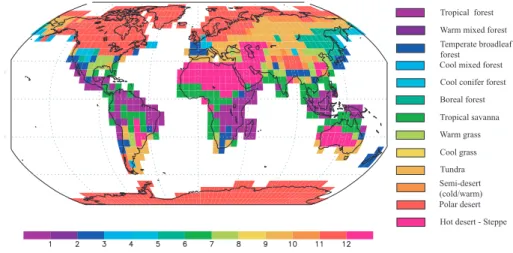
discussed are presented in Fig.4.

1- Siberia. In the model, we simulate the disappearance of much of the present-day boreal forest type which is replaced by a mixture of tundra and cool grass types. The non-glaciated area of the northwestern Alaska and Beringian regions are defined as the tundra biome type. These results are more or less in line with available proxy

20

data, in particular with the Bigelow et al. (2003) compilation which depicts different types of tundra over Bering, a small part of northwestern Canada and northern Siberia, except for two sites in Siberia with Temperate Grassland biome (Bigelow et al.,2003;

Kaplan et al., 2003) which replaces the Siberian cool-mixed/boreal forests existing in the present-day.

25

(14)

CPD

2, 1105–1153, 2006

Printer-friendly Version Interactive Discussion and cool grass types. This reflects the too warm conditions prevailing south of the

Fennoscandian ice-sheet in our simulation. Cool grass is attributed as the dominant biome in southeast Europe. This second part is much in line with the compilation of

Ray and Adams(2001) which depicts southern Europe as being dominated by steppe-like conditions with some trees in the more moist areas, and also with the compilation

5

ofPrentice et al.(2000).

3- In northern Africa, there is a general drying, promoting the southward extension of the desert regions – Sahara type – by 5 to (locally) 11◦, at the expense of the tropical Savanna simulated in the LH CTRL simulation. This result is fairly consistent with the southward extension of the Sahara desert boundary by 5◦ of latitude, as depicted by

10

Prentice et al.(2000) andRay and Adams(2001).

4- The regions of tropical forest in central Africa, although already too small in exten-sion in the LH CTRL simulations, are nevertheless smaller in the LGM simulation, with the disappearance of this particular biome along the Atlantic seaboard. Conversely, the tropical forest cover, too extensive already at present-day on the Indian side, is

15

preserved in our LGM simulation. The shrinking – without disappearance – of the trop-ical forest areas in central-west Africa are in line with current reconstructions (Dupont

et al.,2000;Ray and Adams,2001;Leal,2004), although our simulation of extensive tropical forests on the Indian ocean side is unrealistic. This discrepancy between data and model is also found in south America, and is due to an incorrect representation of

20

the zones of high precipitation in the ECBilt model, promoted on the eastern side of the continents instead of more central regions.

5- Central Asia is a place of great expansion of desert and semi-desert biomes in our LGM simulation with respect to the LH CTRL, with, in particular, the appearance of a great desert in central China, surrounded by a cool grass biome replacing most

25

of the simulated LH CTRL warm grass/cool forest. Some regions of tundra and cold semi-desert slightly expand around the Tibetan plateau. Not many changes are seen in the tropical belt (India, southeast Asia and Indonesia) with respect to the LH CTRL simulation, albeit from slight drying conditions inland in southeast Asia. Japan sees the

(15)

CPD

2, 1105–1153, 2006

Printer-friendly Version Interactive Discussion replacement of a mixture of warm/temperate forest in the LH CTRL simulation with a

complete cover of temperate forest in our simulated LGM. All these features are broadly consistent with the current compilations, although some local discrepancies exist.Ray

and Adams (2001) mention the expansion of deserts in central Asia and the shrinking of tree cover in China. The LGM vegetation of Japan is seen as a mixture of cool mixed

5

forest to temperate forest in the data (Prentice et al.,2000), not inconsistent with our simulated dominance of temperate forest.

6- As already discussed, south of the Laurentide ice-sheet we simulate the cover of tree and grass relatively well according to the proxy data available for these PFTs (Williams, 2002). In terms of inferred biomes, central USA is covered by the “warm

10

grass” biome, whereas reconstructions point to “tundra” (Prentice et al.,2000) or “tem-perate grassland” (Ray and Adams, 2001). In so far as we have no simulated tree cover, we agree with these reconstructions. It raises a question relative to the type of biome (cold/temperate) which would be appropriate there and hence question the mean annual temperature of these regions. On the eastern Atlantic coast we simulate

15

a bioclimatic gradient from “tropical savanna” (in Florida) to “tundra”/“temperate forest” (at the ice-sheet border). In the data these regions are depicted as “open conifer wood-land” in Florida to “taiga” of “cool mixed forest” in the north (Prentice et al.,2000;Ray

and Adams,2001). Therefore, the model exhibits some exaggeratedly warm conditions in southeastern USA with respect to the data, but is not too far off at the ice-sheet

bor-20

der. Towards the Pacific coast, we obtain a mixture of “temperate forest” to “cool conifer forest” with some tundra, compared to “tundra” and “cool conifer” in the data (Prentice

et al.,2000). This area seems therefore quite consistent with the proxy data. South-ward we have a fairly extensive cover of “tropical forest” in Central America, outlining the too humid conditions we simulate there compared to the data (Ray and Adams,

25

2001).

7- In south America, our estimated biomes show two main patterns: a slight north-wards migration of the Amazonian forest by 5 to (locally) 11◦ of latitude and a general drying of the Argentinian and Uruguayan regions (semi-desert and cool grass biomes).

(16)

CPD

2, 1105–1153, 2006

Printer-friendly Version Interactive Discussion These results for the Amazonian forest are in line with proxy data, although the state of

the Amazonian forest at the LGM is still quite controversial (Colinvaux and de Oliveira,

2000;Ray and Adams,2001;Leal,2004, and others). The drying of the southeastern part of south America (and especially of the shelves exposed during the LGM) is seen in the data, and recorded as dust deposits in the Antarctic ice-cores. We also find

5

some areas of desert and semi-desert in south America (Ray and Adams,2001). 8- Finally our simulation of vegetation in Australia shows an important increase of the desert and semi-desert biomes in our LGM simulations at the expense of the for-est cover (LH CTRL), shrunk to the coastline. These results are in good agreement with current reconstructions which show extreme desert in the centre of Australia with

10

overall less forest cover (Ray and Adams,2001;Prentice et al.,2000). 4.2 Land temperatures: permafrost in Europe

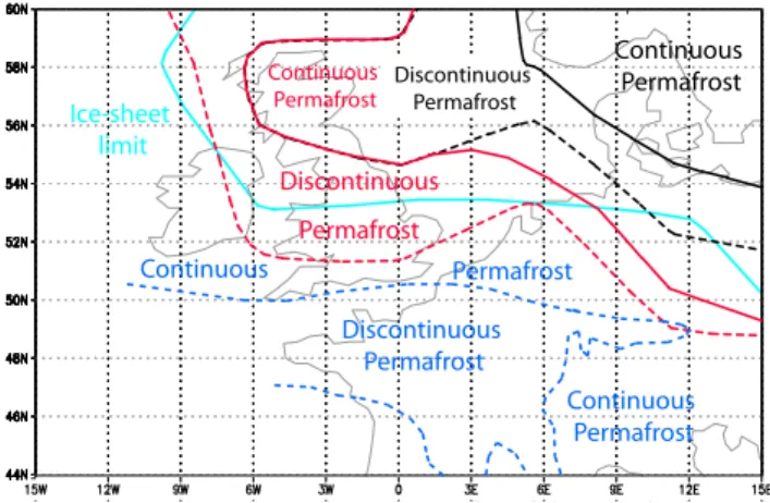
A good indicator of the mean cooling of the climate is the limit of the permafrost. In this paragraph, we therefore try to compare the simulated LGM climate with data for the permafrost limits in Europe, following the types and limits ofRenssen and

Vanden-15

berghe (2003), namely: 1) discontinuous permafrost exits if annual mean temperature is below –4◦C and 2) continuous permafrost exists if both mean annual temperature is below –8◦C and the coldest month temperature is below –20◦C.

Figure5 shows the limits of the continuous and non-continuous permafrost as sim-ulated for the LGM with the limits estimated from the proxy data. It is striking that the

20

simulated area of permafrost is much too small with respect to the proxy data, with continuous permafrost simulated only for Scandinavia and the Baltic States whereas it should extend up to Belgium, the south of Germany and all off the United Kingdom and Ireland (Renssen and Vandenberghe,2003). This underestimation indicates that we overestimate the temperature over western Europe, a feature already noted for the

25

nearby Atlantic ocean. Moreover, we do not simulate continuous permafrost over the British Isles, even if there is a prescribed ice-sheet over their northern reaches. This is probably due, in part, to the resolution of the model: the ice-sheet is prescribed only

(17)

CPD

2, 1105–1153, 2006

Printer-friendly Version Interactive Discussion over a part of the grid-cells in this area, the rest being ocean. Therefore, the

continen-tality is certainly underestimated when close to the oceanic regions (this is also true for other regions like France, Belgium and the Netherlands).

To evaluate how much of the mismatch between model and data is attributable to this continentality effect and to disentangle it from a more global climatic mismatch, we

5

have conducted a sensitivity experiment with a modified land-sea mask for the ECBilt (atmospheric) model. We arbitrarily assigned all grid-cells containing some land a new value of 95% land, to artificially increase the continentality of the more inland points. This set-up leads to some inconsistencies between the atmospheric and oceanic mod-els (ECBilt and CLIO); we therefore only integrate it for 100 years to gain an idea of

10

the atmospheric effect without allowing time to the ocean to be modified. Results are also presented in Fig.5, in terms of permafrost. The limit of continuous permafrost is shifted southwards to the north of The Netherlands and across southern Germany and Ireland. It is not in perfect agreement with the proxy data (especially with the absence of discontinuous permafrost in France) but is nevertheless improved.

15

The southernmost winter sea-ice limit is also modified in this “continentality” experi-ment, from the south of Norway (north of Scotland) to the south of Scotland, along the coast of the United Kingdom. This therefore shows that the relationship between per-mafrost and sea-ice proposed byRenssen and Vandenberghe(2003) in a atmospheric-only model is also found to some extent in a coupled ocean-atmosphere model.

20

The climate of southern Europe still remains too warm with this drastic set-up, im-plying that it depends on the simulated sea surface temperatures (which are not much modified in 100 years). We therefore suggest that simulated sea-surface temperatures are too warm in the eastern north Atlantic in our simulated LGM, as discussed here-after. The method to improve these temperatures is non-trivial, but could encompass

25

(18)

CPD

2, 1105–1153, 2006

Printer-friendly Version Interactive Discussion 4.3 Surface ocean

The goal of this part is to provide a first simple comparison between the MARGO data of the glacial ocean and our simulated LGM state.

4.3.1 Sea-ice distribution

For the northern hemisphere, there is an important increase of the sea-ice area

com-5

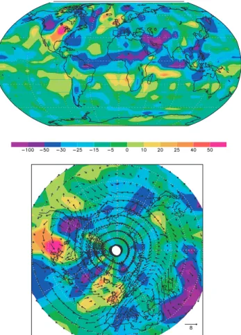
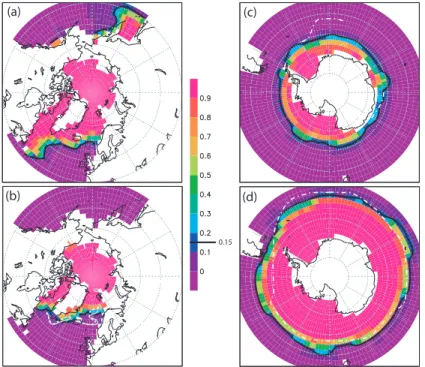
pared to LH CTRL, but in a spatially non-homogeneous fashion (see Fig.6, panels a and b). The summer extent in our simulated LGM is comparable to our present-day winter, with sea-ice covering the Labrador Sea, the Arctic (quasi-continuously) and a small part of the Nordic Seas, almost to the north of Norway. There is also some sea-ice maintained along the coast of Greenland. If compared with the estimations of

10

Kucera et al.(2005b) for the limit of seasonal ice-free conditions, our simulated sea-ice cover agrees fairly well. In particular, we faithfully reproduce the ice-free conditions prevailing over most of the Nordic Seas and the more extensive southwards extent on the western Atlantic, especially along the coast of Greenland. The simulated bo-real winter sea-ice extent shows an important increase of especially along the coast

15

of Newfoundland extending far into the western Atlantic. Conversely, on the eastern side, the winter extension is much more limited, to the south of Iceland and Norway. This shows the effect of the still active north Atlantic drift which, by warming the sur-face waters, enables ice-free conditions in an important part of the eastern Atlantic. The sea-ice cover is probably somewhat underestimated: given the presence of an

20

ice-sheet covering Scotland and the north of Ireland, it is probable that sea-ice also existed there during winter, at least along the coast. Part of the answer probably lies in the coarse resolution of the atmospheric model, T21, a resolution at which the Scottish ice-sheet has a very low altitude. Another reason might be due to the land-sea mask for a model with a relatively low spatial resolution, as already mentioned in4.2.

25

For the southern hemisphere, there is good agreement between the sea-ice concen-trations in our simulated LGM climate and proxy data (Crosta and Pichon, 1998a,b;

(19)

CPD

2, 1105–1153, 2006

Gersonde and Zielinski,2000;Gersonde et al.,2005), as can be seen in Fig.6, panel (d). We overestimate slightly the sea-ice cover occurring at the transition between the Pacific and the Atlantic sector in the Southern Ocean, particularly in the southwest of the Magellan archipelago. We also slightly underestimate the sea-ice cover in the southern Atlantic, but overall the agreement is very good. The simulated sea-ice

con-5

centration for the austral summer is also good in the Indian sector, but not so good for the Atlantic sector. The model captures fairly well the asymmetry between the Indian sector, where the summer sea-ice extent is comparable to today’s, and the Atlantic sector, where it is more extensive. However, it fails to reproduce the large extent of sea-ice between –5 and 5◦W. There are two options to account for this discrepancy:

10

either the limit derived from the diatoms is for the particularly cold summers or there is a spreading of sea-ice which is not represented in the model. The former option, though the sea-ice extent is denoted as “sporadic” (Gersonde et al., 2005), seems however not to be the most probable: Gersonde et al. (2003) rather point to a local expansion due to specific Weddell Sea dynamics, which, we believe, are not represented in the

15

CLIO model.

4.3.2 Sea Surface Temperatures

Here we provide an outline of the data–model comparison between LOVECLIM and MARGO for the annual mean SST and LGM to LH difference, to better position the state of the simulated LGM climate. The MARGO project released an extensive coverage of

20

Sea Surface Temperature (SST) estimates for the LGM for a wide range of proxies. It is beyond the scope of the present study to compare in detail the results obtained here with the MARGO database, especially taking into account that not only annual average SSTs are provided, but also in most cases those for summer and winter (seeKucera

et al. (2005a) and companion papers). We will follow an approach comparing different

25

regions: Indian Ocean and Australian margins, Pacific, Southern and Atlantic Ocean. For the Indian Ocean and the Australian margins, the model indicates differences of –1 to –2◦C relatively homogeneously, in good agreement with proxy data (Barrows and

(20)

CPD

2, 1105–1153, 2006

Printer-friendly Version Interactive Discussion Juggins,2005). Indeed, in terms of mean annual SST anomalies between LGM and

present-day, the proxy data broadly show a general moderate cooling of the equatorial regions of 0 to 3◦C. Some data points for the equatorial Indian ocean even indicate no changes or a small warming. In the tropical regions, the Gulf of Bengal and the Arabian Sea show a very small cooling, with no change or less than 1◦C cooling. This feature is

5

not seen in our simulation, which yields a cooling by 1 to 2◦C, and even some greater cooling along the coast of India. The reason for this mismatch is not clear, and would need to be further investigated. Changes are of greater magnitude in the proxy data to the south, with cooling of 3 to 5◦C at 30–35◦S south of Madagascar. This is also more or less the case in the model, which simulates cooling of 2 to 4◦C in the same

10

area. Around 40◦S, eastward from the Kerguelens, the data show a more pronounced cooling, between 3 and 5◦C; this feature is also well marked in the simulated LGM where cooling reaches 3 to 5◦C. In this region, we find the greatest simulated cooling in the southern hemisphere ocean, with about 8◦C. These huge changes are linked to the northwards migration of the Polar Front and of Antarctic sea-ice, which promote

15

the northward expansion of colder waters. Finally, the biggest changes occur in the Pacific ocean, east of Australia, where there is a cooling of 3 to 5◦C at 30◦S, and up to 7–8◦C over the Campbell Plateau, southeast of New Zeeland. These changes are qualitatively well represented in the model which simulates a –3 to –4◦C change off the eastern coast of Australia, and 4 to 5◦C cooling at the Campbell Plateau. We do not

20

reach the extreme cold shown by the proxy data in the latter region, but the agreement is nevertheless good.

For the nearby Pacific, data are more sparse, but still show some patterns which we can compare to our simulation (Kucera et al.,2005b). The equatorial Pacific, as reconstructed, shows little changes (assigned as –1 to 1◦C), but with slightly cooler

25

temperatures on the south American side (–1 to –3◦C). This is also the case in our simulation, which presents an homogeneous cooling of 0 to 1◦C in the equatorial re-gion, with the exception of slightly cooler temperatures along the south American coast (–1 to –2◦C). We simulate 1 to 2◦C cooling in the Pacific warm pool, quite in line with

(21)

CPD

2, 1105–1153, 2006

Printer-friendly Version Interactive Discussion independent proxy data estimates (Chen et al.,2005). At 30◦N, the reconstructions

show no clear signal (ranging from+1 to –3◦C) to compare to our simulated 2 to 4◦C cooling. Northeast of Japan, around 50◦N, the data show an LGM to LH CTRL cooling of about 1 to 3◦C or even more; our simulation compares relatively well with a –2 to –4◦C changes in this region. Finally, our simulation does not reproduce the cooling of

5

more than 3◦C seen in the proxy data for the American coast at 40◦N. In particular, the proxy data shows an annual mean temperature of about 8◦C at this location whereas the model simulates an annual temperature of about 12 to 14◦C, a temperature barely reached in the proxy data 10◦westward. Two possibilities could be further investigated: the first would be the role of coastal effects, the second of the extension of sea-ice in

10

the northeastern Pacific (non-existent in our simulations, see Fig.6) both in relationship with the evolution of the California current.

Around Antarctica, our model simulates an important cooling, with an annular pattern around the continent, quite in line with the proxy data ofGersonde et al.(2005). This seems a logical counterpart of the good ability of the model to simulate the sea-ice in

15

this region.

For the Atlantic, our simulations produce general changes quite consistent with the proxy data (Pflaumann et al.,2003;Kucera et al.,2005b) for the equator regions (–2 to –4◦C in both data and model) and the 20◦N band (0 to –1◦C in the data vs. –1 to –2◦C in the model. The agreement holds further to the north where the model simulates a

20

cooling from 2◦C at 30◦N to 4◦C around 40◦N, whereas proxy data infer a cooling from –1 to –4◦C. There is however an important mismatch in the more northern regions, where if the anomalies simulated and measured are comparable, they do not occur at the same place: the model simulates the maximum cooling along the American coast whereas this is found off the coast of Ireland according to the proxy. This mismatch may

25

be due to model mis-evaluation of the northern Atlantic gyre circulation, or the treat-ment of the Mediterranean sea, as discussed below. Model–data discrepancies in this area are a common feature already recognised in several coupled models (Kageyama

(22)

CPD

2, 1105–1153, 2006

Printer-friendly Version Interactive Discussion In the Mediterranean sea, although the resolution of the model is too low to simulate

the dynamics occurring here in detail, we obtain a broad agreement with the proxy data (Hayes et al.,2005). We simulate anomalies ranging from –5 to –6◦C in the western part (–6◦C in the data) to –3 to –4◦C in the eastern part (–2 to –3◦C in the data).

To summarise, we obtain a good general agreement between simulated SSTs and

5

anomalies and the proxy data available, with some mismatches in specific regions. The causes of these mismatches may be diverse, but several seem to be linked to the displacement of oceanic fronts or local currents, features difficult to simulate with accuracy. The precise cause of these mismatches should be further investigated; nev-ertheless, we can state that the obtained surface LGM cooling is realistic.

10

4.4 Subsurface northern Atlantic and Nordic seas

Given the importance of the north Atlantic ocean and Arctic Seas in producing part of the deep waters of the world ocean, we perform here a more detailed comparison between the model and the proxy data (Meland et al.,2005), as shown in Fig.8. Our results (panel a) are given on the same projection and scale for ease of comparison

15

with temperatures estimates from δ18O (see panel b, reproduced fromMeland et al.,

2005).

The data presented show a fairly strong east-west gradient, from quite high temper-atures (8 to 9◦C) off the coast of France to much lower temperatures (1 to 3◦C) south of Greenland at the same latitude. This gradient is present all the way to Svalbard, but

20

weakens to a 3◦C difference between east and west along Iceland, similar at the south of the Svalbard. In our simulated LGM, such a gradient also exists (linked to the pres-ence of the (glacial) north Atlantic Drift) but it is of correct magnitude only around the north of Ireland (6◦C difference from 9◦C on the east coast to 3◦C to the west). South of about 50◦N, the model shows fairly homogeneous relatively high annual temperature

25

(more than 10◦C). These waters of quite high temperatures entering the eastern At-lantic originate from a mixture of lower latitude AtAt-lantic waters and Mediterranean sea water of higher temperatures. Due to the relatively coarse resolution of the model, the

(23)

CPD

2, 1105–1153, 2006

Printer-friendly Version Interactive Discussion strait of Gibraltar is much larger than in reality. Therefore, the exchange seems to be

too important at the LGM between the Mediterranean sea and the Atlantic ocean. This is likely to be the source of the 2 to 3◦C overestimation off the coast of Ireland.

Northwards, the model results are fairly comparable to the data, with only about 1◦C difference, and a very similar east-west pattern, indicating that we correctly simulate

5

the entrance of north Atlantic waters in the Nordic Seas. For the Nordic seas, our simulated annual temperatures are more homogeneous than those seen in the data, with slightly too cold temperatures at the northern tip of Norway. This seems to be linked to a small regional overestimation of the sea-ice cover in that area (see Fig.6). Otherwise, the annual temperature in the Nordic Seas is fairly well represented, with

10

waters close to the freezing point along the western coast of Greenland, suggesting perennial sea-ice cover.

To summarise, the model properly simulates the annual mean temperature in the northern Atlantic and Nordic Seas, with a more or less correct east-west gradient. A discrepancy is found in the absolute value south of 55◦N, probably linked to the

15

representation of the Mediterranean outflow in a relatively coarse resolution model. This latter question needs to be re-adressed in future studies.

4.5 Deep ocean circulation

In this paragraph, we review the LGM state as simulated by the LOVECLIM model for the oceanic circulation with respect to the available proxy data. Different types of

20

proxies are usually used as constraints with the view of determining the palaeoceano-graphic state of the LGM.

In terms of location of deep water masses formation, the simulated shift of the north convection site is consistent with proxy data evidence (Labeyrie et al., 1992; Oppo

and Lehman,1993) revealing a southward shift of the location of northern deep water

25

formation. Proxy data evidence also exist for active deep water formation in the Nordic Seas (Dokken and Jansen,1999) during the LGM, in line with our findings.

(24)

CPD

2, 1105–1153, 2006

δ13C measured in foraminifera tests (Duplessy et al., 1988, , for example), used to distinguish between ventilated and less-ventilated water masses. However, it is difficult to compare this to model output when the δ13C itself is not explicitly simulated. Defining the δ13C end-members of the (supposed) main water masses allow to evaluate with some accuracy (Duplessy et al., 1988; Curry and Oppo,2005) the degree of mixing

5

between northern and southern mass contribution. For example, inCurry and Oppo

(2005), a ratio of 50% of GAABW to 50% of GNAIW is found in the north Atlantic at 3100 m and 30◦N), but it is nearly impossible to derive such information from the model output (flow, temperature, salinity fields) without explicit tracer simulation. Moreover, it has been shown that the glacial δ13C distribution poorly constrains the overturning

10

circulation in inverse models (LeGrand and Wunsch, 1995). Therefore, we will not attempt a comparison between the model results and the δ13C distribution obtained from proxy data.

Conversely, Pa/Th ratios measured in the shells of foraminifera, used as a proxy for advection, are linked directly to changes of oceanic circulation. The Pa/Th is a

15

Lagrangian tracer and thus integrates changes in transport of water from the source (sinking regions) to the site where it is measured. Therefore, its recorded variation over time at the site may depend on the global circulation (in average, less water advected in the whole north Atlantic and over the site) or a more local change at the site, being more slowly ventilated whereas some regions are more ventilated. From the three different

20

studies addressing changes in oceanic circulation with the Pa/Th, one (Yu et al.,1996) was aimed at basin scale reconstruction of the LGM oceanic circulation. They showed that the data obtained were consistent with a strength of Atlantic meridional overturning similar to that of present-day. In a later reassessment of the same data with the aid of a model,Marchal et al.(2000) showed that available Pa/Th data is also consistent

25

with a reduction of the strength of the circulation by up to 30%. Finally two recent studies addressed the temporal variation of the thermohaline circulation in the western (McManus et al.,2004) and eastern (Gherardi et al.,2005) Atlantic basins over the last deglaciation. The first one showed that at a depth of 4.5 km in the west Atlantic, the

(25)

CPD

2, 1105–1153, 2006

Printer-friendly Version Interactive Discussion vertically integrated oceanic transport was reduced by 30% at the LGM with respect to

present-day. The second one deduced that the vertically integrated oceanic transport in the eastern Atlantic at a depth of 3.1 km was enhanced at the same time. This indicates that: a) the thermohaline circulation was stronger in the first 3 km of the ocean, a feature compatible with the circulation we obtain in the model and b) that the deep

5

circulation between 3 and 4.5 km was likely to be very sluggish between 30 and 40◦N, a feature also consistent with our simulated meridional overturning circulation (see figure

3). Therefore, although our oceanic circulation pattern might seem to disagree with the “classic” view of the LGM circulation (promoting a much stronger GAABW inflow in the deep Atlantic and a reduced NAIW formation), it appears to be quite consistent with

10

available Pa/Th data constraining the LGM circulation.

Comparison between proxy data and model for the LGM, in terms of temperature and salinity, is generally not possible. However, a few data have been published, based on pore waters measurements in a few sediment cores (Adkins et al., 2002). Table 2

shows a comparison between our simulated LGM ocean and the points measured by

15

Adkins et al. (2002). In proxy data, glacial salinity and temperatures decrease from very high salinities (37.08 permil) and cold waters (–1.3◦C) in the southern Ocean to lower salinities and temperatures toward the north Atlantic ocean. Such changes can be interpreted as the mixing between a cold and extremely saline Southern Ocean water mass (GAABW) and a less saline and extremely cold North Atlantic deep water

20

mass (GNADW).

In the model, we obtain cold Southern Ocean waters (e.g. –1.41◦C in the Pacific sector) but a much warmer deep north Atlantic, indicating too strong an influence of deep waters formed south of Iceland (especially at 2 km depth), whereas the colder water formed in the Nordic Seas should be more dominant. Conversely, we simulate

25

relatively correctly the salinity of the northern water mass, but largely underestimate that of the southern water mass. This shows that we do not form deep waters with the correct properties. The densities we simulate are quasi identical in the north and in the south (difference of +0.06 kg.m-3, in σ₁) whereas they are substantially different

(26)

CPD

2, 1105–1153, 2006

Printer-friendly Version Interactive Discussion in the proxy data (difference of about –1kg.m-3, in σ₁). This might indicate that there

was more presence of GAABW in the north Atlantic in the LGM (southern sourced waters being much denser than northern ones), but the very different characteristics of the two extremes sites measured (ODP 1063 and 1093) shows that there were two different water masses filling the deep Atlantic.

5

To conclude this proxy data – model comparison we can state that although the characteristics of the deep water masses we obtain are substantially different from data inferences (northern sourced being too warm and southern sourced being not saline enough) the circulation pattern is not inconsistent with evidence from the proxy data.

10

5 Sensitivity experiments

5.1 Sensitivity of the simulated LGM to various parameters values

To explore the stability of the oceanic circulation obtained, we have performed an en-semble of sensitivity studies of the LGM state to different parameters intrinsic to the model (see Table3), or dependent on the LGM set-up chosen. For each parameter

15

tested, we restarted from the LGM state and ran the model with the new parameter’s value until equilibrium was reached (usually 1000 or 1500 years, except for runs with importantly modified deep circulation, which need to be run for 3000 years). As we per-formed these experiments in order to determine whether the simulated LGM circulation was a stable feature in the LOVECLIM model or only a stable state for the current set of

20

parameters, the results are expressed in terms of thermohaline circulation intensities for the north Atlantic deep water mass and the Southern Ocean deep water mass.

Generally, we performed three types of sensitivity experiments: those in which we modify the surface water budget by modifying the partitioning of the water coming from land (snow melting, rivers and calving: 2,3,4), those in which the effect of the wind

25

on the sea or sea-ice was modified (5,6,7) and those for which an intrinsic oceanic 1129

(27)

CPD

2, 1105–1153, 2006

Printer-friendly Version Interactive Discussion parameter value was modified (8,9,10).

In the modified freshwater budget experiments, we modified the outlet for the river runoff and calving to increase the input of water to the GIN seas (2), to displace all Arctic outlets into the north Atlantic, south of 50◦N, (3) and modified the redistribution of calving from Antarctica from the border of the continent to 60 to 50◦S. Results

5

obtained for these three experiments showed that the LGM circulation is not sensitive to these small change in the freshwater budget, the maximum effect obtained (3) being of 1.5 Sv on the deep southern water mass entering the Atlantic basin (in response to a slight increase in salinity of these waters, consistent with the discussion of Sect.4.5). In the experiments with modified wind effect on the surface, we integrated the model

10

with three different set-ups: one with a modified drag coefficient (85% of the control value) for the wind on the surface, both for ocean and sea-ice (5), two where we ap-plied drastic changes on the wind-drag coefficient with respect to sea-ice (6 and 7 with respectively 150 and 50% of the control value). These experiments were chosen for two reasons: a) the CLIO ocean model is known to be sensitive to the value of the

15

drag coefficient chosen, b) the sea-ice export is controlled by the wind on sea-ice; an easy way of testing different partitioning of the sea-ice is to modify the effectiveness of wind on the latter. In experiment (5) we obtained very little effect on the water masses from the 15% reduction in the wind-drag coefficient. As expected, there is more sea-ice in the GIN seas, as it is less exported. This larger sea-ice extent promotes a slightly

20

reduced deep water formation in the GIN seas, caused by both the insulation effect of the sea-ice which prevents the cooling of the surface ocean and the reduced salinity increase linked to the formation of sea-ice. The same effect is obtained in experiments (6) and (7) where the drastic reduction of the wind-drag coefficient on sea-ice (6) pro-vokes a quasi-cessation of deep water formation in the GIN seas. This is due to the

25

extremely reduced export of sea-ice thereby considerably reducing the meridional over-turning both for the north Atlantic deep water mass and for the southern deep water mass. The opposite is also valid for experiment (7) where the wind-drag is increased: we obtain an increase of the deep water formation, with a shift in the northern part

(28)

CPD

2, 1105–1153, 2006

Printer-friendly Version Interactive Discussion from the south of Iceland to the Nordic and Labrador seas (present-day like mode of

deep water formation). It should be noted however that a) the effect of changes in this parameter value on the thermohaline circulation is not linear b) there is no change in the relative proportion of our two water masses in the Atlantic.

Finally we also changed some classic intrinsic parameters in the ocean: the

Gent-5

McWilliam coefficient in the isopycnal mixing scheme of the CLIO model (Gent and

Mcwilliams,1990;Goosse and Fichefet,1999) (8, 200% of the control value) and the background diffusivity in the deep ocean (9, 200% of the control value). This latter choice of modified parameters is made as they have been shown to have an effect both on water properties and on the strength of the overturning.

10

To summarise, we can say that none of the parameter modification suggested here could enable a drastic change in the balance between northern and southern deep water masses, but confirm (3) that an increase in salinity of the southern deep water mass tends to increase its presence in the deep Atlantic. This ensemble of tests also shows that the export of sea-ice is an important process in governing the absolute

15

strength of deep water formation in the model (6,7). 5.2 North Atlantic freshwater input sensitivity

A classical test for assessing the oceanic sensitivity to freshwater fluxes is to perform a simulation with a slowly varying additional flux to the north Atlantic and to monitor the effect on the thermohaline circulation (Rahmstorf, 1995). The freshwater flux is

20

here added between 40 and 60◦N in the north Atlantic and varies at a rate of 0.05 Sv per thousand years. A number of coupled models have been used to perform this experiment for the LH climate (including the ECBilt–CLIO model, seeRahmstorf et al.

(2005) for a review), but few coupled models have produced one for glacial boundary conditions. The freshwater sensitivity test presented here is the first to be performed in

25

a 3-D coupled atmosphere-ocean-vegetation model.

Results are presented in Fig.9in terms of NADW export out of the Atlantic, and show the “classic” hysteresis behavior. While adding freshwater to the north Atlantic ocean,

(29)

CPD

2, 1105–1153, 2006

Printer-friendly Version Interactive Discussion there is a transition between an active mode (more than 10 Sv) and a reduced mode

(less than 5 Sv) of the thermohaline circulation (“on” and “off” mode) for an additional freshwater flux of about 0.22 Sv. The flux of thermohaline export at 20◦S then flattens to a small value around 2 Sv. When decreasing the additional freshwater flux to trigger a switch to the “on” mode, the circulation does not bounce back spontaneously, but a

5

small (0.02 Sv) negative freshwater flux is needed. This would indicate that our model presents two stable states under LGM boundary conditions. To further test this hypoth-esis, we computed an additional experiment (not shown), starting from the hysteresis ”off” state with the additional freshwater flux at zero (state corresponding to the inter-sect between the dashed line and the grey branch in Fig.9) and integrating it without

10

additional freshwater flux. After 600 years of integration, the thermohaline circulation switched back to the “on” mode, without the aid of an additional salinity flux. This shows that the ”off” mode in LOVECLIM under LGM boundary conditions is unstable. The natural variability simulated by the model enables the thermohaline circulation to return to the “on” mode. This shows out that the model might also be able to switch

15

back to the “on” state for a small positive additional freshwater flux if time was given to allow for re-equilibration. Thus, the picture of thermohaline sensitivity given in Fig.9is only a quasi-equilibrium view, and the limit fluxes obtained to switch between “on” and “off” are only approximate, being dependent on the rate of additional freshwater flux chosen and on the model natural variability, as expected.

20

To summarise, the LOVECLIM model presents one stable state (the “on” state) and one unstable state (the “off” state) for the thermohaline circulation under LGM boundary conditions. We can also additionally mention that the “off” state is very close to being stable, as is shown by the broad hysteresis pattern obtained here.

6 Summary and conclusions

25

In this study, we have presented the LGM climate simulated by the LOVECLIM Earth system model, from atmospheric, oceanic and vegetation points of view. The