HAL Id: hal-00851658
https://hal.inria.fr/hal-00851658
Submitted on 19 Aug 2013
HAL is a multi-disciplinary open access
archive for the deposit and dissemination of
sci-entific research documents, whether they are
pub-lished or not. The documents may come from
teaching and research institutions in France or
abroad, or from public or private research centers.
L’archive ouverte pluridisciplinaire HAL, est
destinée au dépôt et à la diffusion de documents
scientifiques de niveau recherche, publiés ou non,
émanant des établissements d’enseignement et de
recherche français ou étrangers, des laboratoires
publics ou privés.
Gabriel Scherer, Jan Hoffmann
To cite this version:
Gabriel Scherer, Jan Hoffmann. Tracking Data-Flow with Open Closure Types. [Research Report]
RR-8345, INRIA. 2013, pp.24. �hal-00851658�
ISSN 0249-6399 ISRN INRIA/RR--8345--FR+ENG
RESEARCH
REPORT
N° 8345
August 2013 Project-Team GalliumTypes ouverts de
fermetures, et une
application au typage des
flots de données
RESEARCH CENTRE PARIS – ROCQUENCOURT
Domaine de Voluceau, - Rocquencourt B.P. 105 - 78153 Le Chesnay Cedex
application au typage des flots de données
Gabriel Scherer, Jan Hoffmann
*
Équipe-Projet Gallium
Rapport de recherche n° 8345 — August 2013 —24pages
Résumé : Les systèmes de types cachent les variables capturées par une fermeture, et ce dès sa création. À un point donné du programme, il serait en fait possible de mentionner certaines de ces variables, celles qui sont toujours présentes dans l’environnement lexical de typage. Ce raffinement des types de fermetures, plus “ouverts” car mentionnant le contexte qui les entoure, est désirable pour certaines applications des systèmes de types à l’analyse de programmes.
Cet article introduit formellement de tels types ouverts de fermetures, pour mettre à plat leur traitement théorique recélant quelques difficultés techniques : le type d’une fermeture mentionne ses dépendances sur le contexte, et varie donc selon les différents point du programme.
En guise d’exemple, ils sont utilisés pour garder trace des informations de typage de flots de données induits par la capture des valeurs de l’environnement dans les fermetures.
Un prototype d’implémentation de ce système de types est publiquement disponible.
Mots-clés : typage, fermetures, types ouverts
Abstract : Type systems hide data that is captured by function closures in function types. In most cases this is a beneficial design that enables simplicity and compositionality. However, some applications require explicit information about the data that is captured in closures.
This paper introduces open closure types, that is, function types that are deco-rated with type contexts. They are used to track data-flow from the environment into the function closure. A simply-typed lambda calculus is used to study the pro-perties of the type theory of open closure types. A distinctive feature of this type theory is that an open closure type of a function can vary in different type contexts. To present an application of the type theory, it is shown that a type derivation es-tablishes a simple non-interference property in the sense of information-flow theory. A publicly available prototype implementation of the system can be used to expe-riment with type derivations for example programs.
Contents
1 Introduction 3
1.0.1 Related Work . . . 5
2 A Type System for Open Closures 5
2.0.2 A Term Language, and a Naive Attempt at a Type System . 7
2.0.3 Maintaining Closure Contexts. . . 8
2.0.4 On open closure types on the left of function types . . . 12
3 A Big-Step Operational Semantics 13
3.0.5 Values and Value Substitution . . . 13
3.0.6 Substituting Values . . . 14
3.0.7 The Big-Step Reduction Relation . . . 16
4 Dependency information as non-interference 19
5 Prototype implementation 22
6 Conclusion 23
1
Introduction
Function types in traditional type systems only provide information about the arguments and return values of the functions but not about the data that is captured in function closures. Such function types naturally lead to simple and compositional type systems.
Recently, syntax-directed type systems have been increasingly used to statically verify strong program properties such as resource usage [LP13, JHLH10, HAH12], information flow [HR98,SM03], and termination [Abe08,CK01,BGR08]. In such type systems, it is sometimes necessary and natural to include information in the function types about the data that is captured by closures. To see why, assume that we want to design a type system to verify resource usage. Now consider for example the curried append function for integer lists which has the following type in OCaml.
append: int list→ int list → int list
At first glance, we might say that the time complexity of append is O(n) if n is the length of the first argument. But a closer inspection of the definition of append reveals that this is a gross simplification. In fact, the complexity of the partial function call app_par = append ℓ is constant. Moreover, the complexity of the
functionapp_par is linear—not in the length of the argument but in the length of the list ℓ that is captured in the function closure.
In general, we have to describe the resource consumption of a curried function
f : A1→ · · · → An→ A with n expressions ci(a1, . . . , ai) such that cidescribes the
complexity of the computation that takes place after f is applied to i arguments
a1, . . . , ai. We are not aware of any existing type system that can verify a statement
of this form.
To express the aforementioned statement in a type system, we have to decorate the function types with additional information about the data that is captured in a function closure. It is however not sufficient to directly describe the complexity of a closure in terms of its arguments and the data captured in the closure. Admittedly, this would work to accurately describe the resource usage in our example function appendbecause the first argument is directly captured in the closure. But in general, the data captured in a closure f a1· · · aican be any data that is computed from the
arguments a1, . . . , ai (and from the data in the environment). To reference this
data in the types would not only be meaningless for a user, it would also hamper the compositionality of the type system. It is for instance unclear how to define subtyping for closures that capture different data (which is, e.g., needed in the two branches of a conditional.)
To preserve the compositionality of traditional type systems, we propose to describe the resource usage of a closure as a function of its argument and the data that is visible in the current environment. To this end we introduce open closure
types, function types that refer to their arguments and to the data in the current
environment.
More formally, consider a typing judgment of the form Γ⊢ e : σ, in a type system
that tracks fine-grained intensional properties characterizing not only the shape of values, but the behavior of the reduction of e into a value (e.g., resource usage). A typing rule for open closure types, Γ, ∆ ⊢ e : [Γ′](x:σ) → τ, captures the idea
that, under a weak reduction semantics, the computation of the closure itself, and later the computation of the closure application, will have very different behaviors, captured by two different typing environments Γ and Γ′ of the same domain, the free variables of e. To describe the complexity ofappend, we might for instance have a statement
ℓ:int list⊢append ℓ : [ℓ:int list](y:int list)→ int list .
This puts us in a position to use type annotations to describe the resource usage of appendℓ as a function of ℓ and the future argument y. For example, using type-based
amortized analysis [HAH12], we can express a bound on the number of created list notes inappendwith the following open closure type.
append: [](x:int list0)→ [x:int list1](y:int list0)→ int list0.
The intuitive meaning of this type for append is as follows. To pay for the cons operations in the evaluation of appendℓ1 we need 0·|ℓ1| resource units and to pay
for the cons operations in the evaluation ofappendℓ1ℓ2we need 0·|ℓ1|+1·|ℓ2| resource
units.
The development of a type system for open closure types entails some interesting technical challenges: term variables now appear in types, which requires mechanisms for scope management not unlike dependent type theories. If x appears in σ, the context Γ, x:τ, y:σ is not exchangeable with Γ, y:σ, x:τ . Similarly, the judgment Γ, x:τ ⊢ e2 : σ will not entail Γ ⊢ letx = e1ine2 : σ, as the return type σ may
contain open closures scoping over x, so we need to substitute variables in types. The main contribution of this paper is a type theory of open closure types and the proof of its main properties. We start from the simply-typed lambda calculus, and consider the simple intensional property of data-flow tracking, annotating each simply-typed lambda-calculus type with a single boolean variable. This allows us to study the metatheory of open closure types in clean and straightforward way. This is the first important step for using such types in more sophisticated type systems for resource usage and termination.
Our type system for data-flow tracking captures higher-order data-flow infor-mation. As a byproduct, we get our secondary contribution, a non-interference property in the sense of information flow theory: high-level inputs do not influence the (low-level) results of computations.
To experiment with of our type system, we implemented a software prototype in OCaml (see Section 5).
1.0.1 Related Work
In our type system we maintain the invariant that open closure types only refer to variables that are present in the current typing context. This is a feature that distinguishes open closure types from existing formalisms for closure types.
Contextual types [NPP08,PD08,SS12] also decorate types with context infor-mation. However, it is not necessary in contextual modal type theory that the context that is captured in a type is related to the current context. Furthermore, our goal of describing properties that may depend on previous function arguments and other visible variables is quite different from the main applications of con-textual types in programming language support for manipulating proof terms and meta-variables.
Having closure types carry a set of captured variables has been done in the literature, as for example in Leroy [Ler92], which use closure types to keep track of of dangerous type variables that can not be generalized without breaking type safety, or in the higher-order lifetime analysis of Hannan et al. [HHLN97], where variable sets denote variables that must be kept in memory. However, these works have no need to vary function types in different typing contexts and subtyping can be defined using set inclusion, which makes the metatheory significantly simpler. On the contrary, our scoping mechanism allows to study more complex properties, such as value dependencies and non-interference.
The classical way to understand value capture in closures in a typed way is through the typed closure conversion of Minamide et al. [MMH96]. They use ex-istential types to account for hidden data in function closures without losing com-positionality, by abstracting over the difference between functions capturing from different environments. Our system retains this compositionality, albeit in a less apparent way: we get finer-grained information about the dependency of a closure on the ambient typing environment. Typed closure conversion is still possible, and could be typed in a more precise way, abstracting only over values that are outside the lexical context.
Petricek et al. [POM12] study coeffects systems with judgments of the form
CrΓ⊢ e : τ and function types Csσ → τ, where r and s are coeffect annotations
over a indexed comonad C. Their work is orthogonal to the present one as they cover very different topics: on one side, the comonadic semantics structure of coarse-grained effect indexes, and on the other the syntactic scoping rules that arise from tracking each variable of the context separately. We believe that our dependency of types on term variables would make a semantic study significantly more challenging, and conversely that use cases of open closure types are not in general characterized by a comonadic structure.
The non-interference property that we prove is different from the usual treatment in type systems for information flow like the SLam Calculus [HR98]. In SLam, the information flow into closure is accounted for at abstraction time. In contrast, we account for the information flow into the closure at application time.
2
A Type System for Open Closures
We define a type system for the simplest problem domain that exhibits a need for open closure types. Our goal is to determine statically, for an open term e, on which variables of the environment the value of e depends.
We are interested in weak reduction, and assume a call-by-value reduction strat-egy. In this context, an abstraction λx.e is already a value, so reducing it does not depend on the environment at all. More generally, for a term e evaluating to a function (closure), we make a distinction between the part of the environment the
Scope-Context-Nil ∅ ⊢ Scope-Context Γ⊢ σ Γ, x:σ⊢ Scope-Atom Γ⊢ Γ⊢ α Scope-Product Γ⊢ τ1 Γ⊢ τ2 Γ⊢ τ1∗ τ2 Scope-Closure Γ0, Γ1⊢ Γ0⊢ σ Γ0, x:σ⊢ τ Γ0, Γ1⊢ [ΓΦ0](x:σ ϕ)→ τ
Figure 1: Well-scoping of types and contexts
reduction of e depends on, and the part that will be used when the resulting clo-sure will be applied. For example, the term (y, λx.z) depends on the variable y at evaluation time, but will not need the variable z until the closure in the right pair component is applied.
This is where we need open closure types. Our function types are of the form [ΓΦ](x:σϕ) → τ, where the mapping Φ from variables to Booleans indicates on
which variables the evaluation depends at application time. The Boolean ϕ indicates whether the argument x is used in the function body. We call Φ the dependency annotation of Γ. Our previous example would for instance be typed as follows.
y:σ1, z:τ0⊢ (y, λx.z) : σ ∗ ([y:σ0, z:τ1](x:ρ0)→ τ)
The typing expresses that the result of the computation depends on the variable y but not on the variable z. Moreover, result of the function in the second component of the pair depends on z but not on y.
In general, types are defined by the following grammar.
Types∋ σ, τ, ρ ::= types
| α atoms
| τ1∗ τ2 products
| [ΓΦ](x:σϕ)→ τ closures
The closure type [ΓΦ](x:σϕ)→ τ binds the new argument variable x, but not the
variables occurring in Γ which are reference variables bound in the current typing context. Such a type is well-scoped only when all the variables it closes over are actually present in the current context. In particular, it has no meaning in an empty context, unless Γ is itself empty.
We define well-scoping judgments on contexts (Γ ⊢) and types (Γ ⊢ σ). The
judgments are defined simultaneously in Figure1 and refer to each another. They use non-annotated contexts: the dependency annotations characterize data-flow information of terms, and are not needed to state the well-formedness of static types and contexts.
Notice that the closure contexts appearing in the return type of a closure, τ in our rule Scope-Closure, may capture the variable x corresponding to the function argument, which is why we chose the dependent-arrow–like notation (x:σ) → τ
rather than only σ → τ. There is no dependency of types on terms in this system, this is only used for scope tracking.
Note that Γ⊢ σ implies Γ ⊢ (as proved by direct induction until an atom or a
function closure is reached). Note also that a context type [Γ0](x:σ)→ τ is
well-scoped in any larger environment Γ0, Γ1: the context information may only mention
variables existing in the typing context, but it need not mention all of them. As a result, well-scoping is preserved by context extension: if Γ0⊢ σ and Γ0, Γ1⊢, then
Var Γ, x:σ, ∆⊢ Γ0, x:σ1, ∆0⊢ x : σ Product ΓΦ1 ⊢ e 1: τ1 ΓΦ2 ⊢ e2: τ2 ΓΦ1+Φ2 ⊢ (e 1, e2) : τ1∗ τ2 Proj ΓΦ⊢ e : τ1∗ τ2 ΓΦ⊢ πi(e) : τi Lam ΓΦ, x:σϕ⊢ t : τ Γ0⊢ λx.t : [ΓΦ](x:σϕ)→ τ Fix ΓΦ, f :([ΓΨ](x:σϕ)→ τ)χ, x : σϕ⊢ e : τ Γ0⊢fixf x.e : [ΓΨ](x:σϕ)→ τ App-Tmp (Γ0, Γ1)Φfun⊢ t : [Γ Φ clos 0 ](x:σ ϕ)→ τ (Γ 0, Γ1)Φarg ⊢ u : σ
(Γ0, Γ1)Φfun+Φclos+ϕ.Φarg⊢ t u : τ
Let-Tmp
ΓΦdef ⊢ e1: σ ΓΦbody, x:σϕ⊢ e2: τ
Γϕ.Φdef+Φbody ⊢letx = e1ine2: τ
Figure 2: Naive rules for the type system
2.0.2 A Term Language, and a Naive Attempt at a Type System
Our term language, is the lambda calculus with pairs, let bindings and fixpoints. This language is sufficient to discuss the most interesting problems that arise in an application of closure types in a more realistic language.
Terms∋ t, u, e ::= terms
| x variables
| (e1, e2) pairs
| πi(e) projections (i∈ {1, 2})
| λx.e lambda abstractions
| t u applications
| letx = e1ine2 let declarations
For didactic purposes, we start with an intuitive type system presented in Fig-ure 2. The judgment ΓΦ ⊢ e : σ means that the expression e has type σ, in the
context Γ carrying the intensional information Φ. Context variable mapped to 0 in Φ are not used during the reduction of e to a value. We will show that the rules App-Tmp and Let-Tmpare not correct, and introduce a new judgment to develop correct versions of the rules.
In a judgment Γ0 ⊢ λx.t : [ΓΦ](x:σ0) → τ, Γ is bound only in one place (the
context), and α-renaming any of its variable necessitates a mirroring change in its right-hand-side occurrences (ΓΦbut also in σ and τ ), while x is independently bound
in the term and in the type, so the aforementioned type is equivalent to [ΓΦ](y:σ)→
τ [y/x]. In particular, variables occurring in types do not reveal implementation
details of the underlying term.
The syntax ϕ.Φ used in theApp-TmpandLet-Tmprules is a product, or conjunc-tion, of the single boolean dependency annotation ϕ, and of the vector dependency annotation Φ. The sum Φ1+ Φ2 is the disjunction. In theLet-Tmprule for
exam-ple, if the typing of e2determines that the evaluation of e2does not depend on the
definition x = e1(ϕ is 0), then ϕ.Φdefwill mark all the variables used by e1 as not
needed as well (all 0), and only the variables needed by e2 will be marked in the
result annotation ϕ.Φdef+ Φbody.
In the introduction we present closure types of the form [Γ](x:σ)→ τ, while we
here use the apparently different form [ΓΦ](x:σϕ)→ τ. This new syntax is actually
a simpler special case of the previous one: we could consider a type grammar of the form σϕ, and the type [Γ](x:σ)→ τ would then capture all the needed information,
as each type in Γ would come with its own annotation. Instead, we don’t embed dependency information in the types directly, and use annotated context ΓΦto carry
equivalent information. This simplification makes it easier to control the scoping correctness: it is easier to notice that ΓΦand ΓΨare contexts ranging over the same
domain than if we wrote Γ and Γ′. It is made possible by two specific aspects of this simple system:
– Our intensional information has a very simple structure, only a boolean, that does not apply to the types in depth. The simplification would not work, for example, in a security type system where products could have components of different security levels (τl∗ σr), but the structure of the rules would remain
the same.
– In this example, we are interested mostly in intensional information on the contexts, rather than the return type of a judgment. The general case rather suggests a judgment of the form ΓΦ⊢ e : σϕ, but with only boolean
annota-tions this boils to a judgment ΓΦ⊢ e : σ1, when we are interested in the value
being type-checked, and a trivial judgment Γ0 ⊢ e : σ0, used to type-check
terms that will not be used in the rest of the computation, and which degen-erates to a check in the simply-typed lambda-calculus. Instead, we define a single judgment ΓΦ⊢ e : σ corresponding to the case where ϕ is 1, and use the
notation ϕ.Φ to nullify the dependency information coming of from e when the outer computation does not actually depend on it (ϕ is 0).
While dependency annotations make the development easier to follow, they do not affect the generality of the type theory, as the common denominator of open closure type systems is more concerned with the scoping of closure contexts than the structure of the intensional information itself.
2.0.3 Maintaining Closure Contexts
As pointed out, the ruleApp-TmpandLet-Tmpof the system above are wrong (hence the “temporary” name): the left-hand-side of the rule App-Tmp assumes that the closure captures the same environment Γ that it is computed in. This property is initially true in the closure of the rule Lam, but is not preserved by Let-Tmp (for the body type) orApp-Tmp (for the return type). This means that the intensional information in a type may become stale, mentioning variables that have been removed from the context. We will now fix the type system to never mention unbound variables.
We need a closure substitution mechanism to explain the type τf = [ΓΦ, y:ρχ](x:σϕ)→
τψ of a closure f in the smaller environment Γ, given dependency information for
y in Γ. Assume for example that y was bound in a let binding let y = e . . . and
that the type τf leaves the scope of y. Then we have to adapt the type rules to
express the following. “If f depends on y (at application time) then f depends on the variables of Γ that e depends on.”
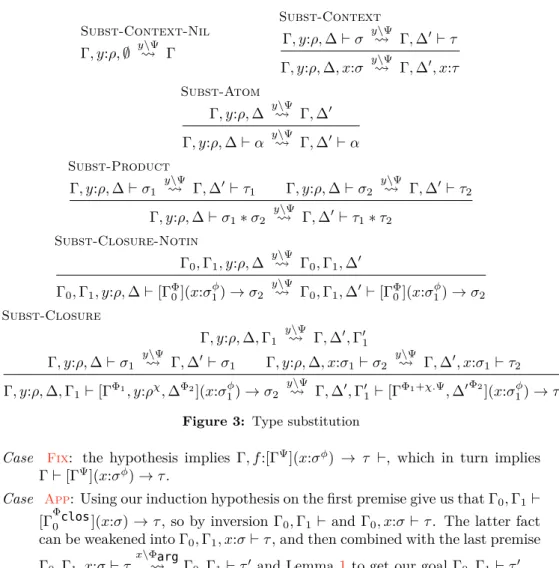
We define in Figure3the judgment Γ, y:ρ, ∆⊢ σ y⇝ Γ, ∆\Ψ ′ ⊢ τ. Assuming that
the variable y in the context Γ, y:ρ, ∆ was let-bound to an definition with usage information ΓΨ, this judgment transforms any type σ in this context in a type τ
in a context Γ, ∆′ that does not mention y anymore. Note that ∆ and ∆′ have the same domain, only their intensional information changed: any mention of y in a closure type of ∆ was removed in ∆′. Also note that Γ, y:ρ, ∆ and Γ, ∆′, or σ and τ , are not annotated with dependency annotations themselves: this is only a scoping transformation that depends on the dependency annotations of y in the closures of
σ and ∆.
As for the scope-checking judgment, we simultaneously define the substitutions on contexts themselves Γ, y:ρ, ∆ y⇝ Γ, ∆\Ψ ′. There are two rules for substituting
a closure type. If the variable being substituted is not part of the closure type context (rule Subst-Closure-Notin), this closure type is unchanged. Otherwise (rule Subst-Closure) the substitution is performed in the closure type, and the neededness annotation for y is reported to its definition context Γ0.
The following lemma verifies that this substitution preserves well-scoping of contexts and types.
Lemma 1 (Substitution preserves scoping) If Γ, y:ρ, ∆ ⊢ and Γ, y:ρ, ∆ y⇝\Ψ Γ, ∆′ hold, then Γ, ∆′ ⊢ holds. If Γ, y:ρ, ∆ ⊢ σ and Γ, y:ρ, ∆ ⊢ σ y⇝ Γ, ∆\Ψ ′ ⊢ τ
hold, then Γ, ∆′⊢ τ holds.
By mutual induction on the judgments Γ, y:ρ, ∆ y⇝ Γ, ∆\Ψ ′ and
Γ, y:ρ, ∆⊢ σ y⇝ Γ, ∆\Ψ ′ ⊢ τ.
Case Subst-Context-Nil: using Scope-Context-Nil, Γ, x:σ ⊢ implies Γ ⊢ σ,
which in turn implies Γ⊢.
Case Subst-Context: from our hypothesis Γ, y:ρ, ∆, x:σ⊢ we deduce Γ, y:ρ, ∆ ⊢ σ.
By induction we can deduce Γ, ∆′ ⊢ τ, which gives context well-formedness
Γ, ∆′ ⊢.
Case Subst-Atom: direct byScope-Atomand induction hypothesis.
Case Subst-Product: by inversion, the last rule of the derivation of Γ, y:ρ ⊢
(σ1∗ σ2) is Scope-Product, so we can proceed by direct induction on the
premises of both judgments.
Case Subst-Closure: Using our induction hypothesis on Γ, y:ρ, ∆, Γ1
y\Ψ
⇝ Γ, ∆′, Γ′
1
we can deduce that Γ, ∆′, Γ′1⊢ and in particular Γ, ∆′⊢.
By inversion, the last rule of the derivation of Γ, y:ρ, ∆, Γ1⊢ [ΓΦ1, y:ρχ, ∆Φ2](y : σ
ϕ1
1 )→
σ2 isScope-Closure. Its premises are Γ, y:ρ, ∆⊢ σ1 and Γ, y:ρ, ∆, x:σ1⊢ σ2,
from which we deduce by induction hypothesis Γ, ∆′⊢ τ1 and Γ, ∆′, x:τ1⊢ τ2
respectively, allowing to deduce that Γ, ∆′ ⊢ [ΓΦ1+χ.Ψ, ∆′Φ2](x : τ
1) → τ2,
which allows to conclude by weakening with the well-scoped Γ′1.
Case Subst-Closure-Notin: direct by induction and inversion. We can now give the correct rules for binders:
Let
ΓΦdef⊢ e1: σ ΓΦbody, x:σϕ⊢ e
2: τ Γ, x:σ⊢ τ
x\Φdef
⇝ Γ ⊢ τ′
Γϕ.Φdef+Φbody⊢letx = e1ine2: τ′ App (Γ0, Γ1)Φfun⊢ t : [Γ Φ clos 0 ](x:σ ϕ)→ τ (Γ0, Γ1) Φarg ⊢ u : σ Γ0, Γ1, x:σ⊢ τ x\Φarg ⇝ Γ0, Γ1⊢ τ′ (Γ0, Γ1) Φ
fun+Φclos+ϕ.Φarg⊢ t u : τ′
Lemma 2 (Typing respects scoping) If Γ⊢ t : σ holds, then Γ ⊢ σ holds.
This lemma guarantees that we fixed the problem of stale intensional informa-tion: types appearing in the typing judgment are always well-scoped.
By induction on the derivation of Γ⊢ t : σ.
Case Var: from the premise Γ0, x : σ1, ∆0⊢ we have Γ ⊢ σ.
Case Prod: direct by induction.
Case Proj: the induction hypothesis is Γ⊢ τ1∗ τ2, from which we get Γ⊢ τi (for
i∈ {1, 2}) by inversion.
Case Lam: the induction hypothesis is Γ, x:σ ⊢ τ. From this we get Γ, x:σ and
Subst-Context-Nil Γ, y:ρ,∅ y⇝ Γ\Ψ Subst-Context Γ, y:ρ, ∆⊢ σ y⇝ Γ, ∆\Ψ ′⊢ τ Γ, y:ρ, ∆, x:σ y⇝ Γ, ∆\Ψ ′, x:τ Subst-Atom Γ, y:ρ, ∆ y⇝ Γ, ∆\Ψ ′ Γ, y:ρ, ∆⊢ α y⇝ Γ, ∆\Ψ ′⊢ α Subst-Product Γ, y:ρ, ∆⊢ σ1 y\Ψ ⇝ Γ, ∆′⊢ τ 1 Γ, y:ρ, ∆⊢ σ2 y\Ψ ⇝ Γ, ∆′ ⊢ τ 2 Γ, y:ρ, ∆⊢ σ1∗ σ2 y\Ψ ⇝ Γ, ∆′⊢ τ 1∗ τ2 Subst-Closure-Notin Γ0, Γ1, y:ρ, ∆ y\Ψ ⇝ Γ0, Γ1, ∆′ Γ0, Γ1, y:ρ, ∆⊢ [ΓΦ0](x:σ ϕ 1)→ σ2 y\Ψ ⇝ Γ0, Γ1, ∆′ ⊢ [ΓΦ0](x:σ ϕ 1)→ σ2 Subst-Closure Γ, y:ρ, ∆, Γ1 y\Ψ ⇝ Γ, ∆′, Γ′ 1 Γ, y:ρ, ∆⊢ σ1 y\Ψ ⇝ Γ, ∆′⊢ σ 1 Γ, y:ρ, ∆, x:σ1⊢ σ2 y\Ψ ⇝ Γ, ∆′, x:σ 1⊢ τ2 Γ, y:ρ, ∆, Γ1⊢ [ΓΦ1, y:ρχ, ∆Φ2](x:σϕ1)→ σ2 y\Ψ ⇝ Γ, ∆′, Γ′ 1⊢ [Γ Φ1+χ.Ψ, ∆′Φ2 ](x:σϕ1)→ τ2
Figure 3: Type substitution
Case Fix: the hypothesis implies Γ, f :[ΓΨ](x:σϕ) → τ ⊢, which in turn implies
Γ⊢ [ΓΨ](x:σϕ)→ τ.
Case App: Using our induction hypothesis on the first premise give us that Γ0, Γ1⊢
[ΓΦ0clos](x:σ)→ τ, so by inversion Γ0, Γ1⊢ and Γ0, x:σ ⊢ τ. The latter fact
can be weakened into Γ0, Γ1, x:σ⊢ τ, and then combined with the last premise
Γ0, Γ1, x:σ⊢ τ
x\Φarg
⇝ Γ0, Γ1⊢ τ′ and Lemma 1to get our goal Γ0, Γ1⊢ τ′.
Case Let: reasoning similar to the App case. By induction on the middle premise, we have Γ, x:σ⊢ τ, combined with the right premise Γ, x:σ ⊢ τ x\Φ⇝ Γ ⊢ τdef ′
we get Γ⊢ τ′.
It is handy to introduce a convenient derived notation ΓΦ ⊢ τ y⇝ Γ\Ψ ′Φ′ ⊢ τ′
that is defined below. This substitution relation does not only remove y from the open closure types in Γ, it also updates the dependency annotation on Γ to add the dependency Ψ, corresponding to all the variables that y depended on – if it is itself marked as needed.
Γ, y:ρ, ∆⊢ τ y⇝ Γ, ∆\Ψ ′⊢ τ′ ΓΦ1, y:ρχ, ∆Φ2⊢ τ y⇝ Γ\Ψ Φ1+χ.Ψ, ∆′Φ2⊢ τ′
It is interesting to see that substituting y away in ΓΦ1, y:ρ, ∆Φ2 changes the
annotation on Γ, but not its types (Γ is unchanged in the output as its types may not depend on y), while it changes the types in ∆ but not its annotation (Φ2 is
unchanged in the output as a value for y may only depend on variables from Γ, not ∆).
The following technical results allow us to permute substitutions on unrelated variables. They will be used in the typing soundness proof of the next section (The-orem 1).
Lemma 3 (Confluence) If Γ1 ⊢ τ1
xa\Ψa
⇝ Γ2a ⊢ τ2a and Γ1 ⊢ τ1
xb\Ψb
⇝ Γ2b ⊢ τ2b
then there exists a unique Γ3⊢ τ3 such that
Γ2a⊢ τ2a
xb\(Ψb+Ψa.Ψb(xa))
⇝ Γ3⊢ τ3 and Γ2b⊢ τ2b
xa\(Ψa+Ψb.Ψa(xb))
⇝ Γ3⊢ τ3
Without loss of generality we can assume that xa appears before xb in Γ1, so in
particular Ψa(xb) = 0. For any subcontext of the form
∆1Ψ1, xa:σaρa, ∆2Ψ2, xb:σbρb
, assume that substituting Ψa for xa first results in
∆1Ψ1+ρa.Ψa, ∆2aΨ2, xb:σbaρb
, while substituting Ψb for xb first results in
∆1Ψ1+ρb.Ψb(∆1), xa:σaρa+ρb.Ψb(xa), ∆2Ψ2+ρb.Ψb(∆2) . Substituting Ψb+ Ψa.Ψb(xa) for xb in ∆1Ψ1+ρa.Ψa, ∆2aΨ2, xb:σbaρb results in ∆1Ψ1+ρa.Ψa+ρb.(Ψb+Ψa.Ψb(xa))(∆1), ∆2aΨ2+ρb.(Ψb+Ψa.Ψb(xa))(∆2a) which simplifies to ∆1Ψ1+ρa.Ψa+ρb.Ψb(∆1)+ρb.Ψb(xa).Ψa, ∆2aΨ2+ρb.Ψb(∆2a) Substituting Ψa+ Ψb.Ψa(xb) = Ψa for xa in ∆1Ψ1+ρb.Ψb(∆1), xa:σaρa+ρb.Ψb(xa), ∆2Ψ2+ρb.Ψb(∆2) results in ∆1Ψ1+ρb.Ψb(∆1)+(ρa+ρb.Ψb(xa)).Ψa), ∆2aΨ2+ρb.Ψb(∆2) which simplifies to ∆1Ψ1+ρb.Ψb(∆1)+ρa.Ψa+ρb.Ψb(xa).Ψa, ∆2aΨ2+ρb.Ψb(∆2)
Given that ∆2and ∆2ahave the same domain (only different types), the
restric-tions Ψb(∆2) and Ψb(∆2a) are equal, allowing to conclude that the two substitutions
indeed end in the same sequent
∆1Ψ1+(ρa+ρb.Ψb(xa)).Ψa+ρb.Ψb(∆1), ∆2aΨ2+ρb.Ψb(∆2)
Note that we can make sense, informally, of this resulting sequent. The variable used by this final contexts are
– the variables used of ∆1 used in the initial judgment (Ψ1)
– the variables of ∆2 (updated in ∆2a to remove references to the substituted
variable xa) used in the initial judgment (Ψ2)
– the variables used by Ψb, if it is used (ρb is 1)
– the variables used by Ψa if either x was used (ρa is 1), or if xb is used (ρb is
1) and itself uses xa (Ψb(xa) is 1).
To get this intuition, we considered again the annotations as booleans, but note that the equivalence proof was done in a purely algebraic manner. It should therefore be preserved in future work where the intensional information has a richer structure.
Corollary 1 (Reordering of substitutions) If Ψa and Ψb have domain Γ, and
Γ1Φ1 ⊢ τ1
xa\Ψa
⇝ Γ2Φ2⊢ τ2
xb\(Ψb+Ψb(xa).Ψa)
⇝ Γ3Φ3 ⊢ τ3
then there exists Γ′2Φ
′ 2⊢ τ′ 2 such that Γ1Φ1⊢ τ1 xb\Ψb ⇝ Γ′ 2 Φ′2 ⊢ τ′ 2 xa\(Ψa+Ψa(xb).Ψb) ⇝ Γ3Φ3 ⊢ τ3
2.0.4 On open closure types on the left of function types
Note that theSubst-Closurehandles the function type on the left-hand-side of the arrow, σ1, is a specific and subtle way: it must be unchanged by the substitution
judgment. Under a slightly simplified form, the judgment reads: Γ, y:ρ, ∆⊢ σ1 y\Ψ ⇝ Γ, ∆′⊢ σ 1 Γ, y:ρ, ∆, x:σ1⊢ σ2 y\Ψ ⇝ Γ, ∆′, x:σ 1⊢ τ2 Γ, y:ρ, ∆⊢ [ΓΦ1, y:ρχ, ∆Φ2](x:σϕ 1)→ σ2 y\Ψ ⇝ Γ, ∆′⊢ [ΓΦ1+χ.Ψ, ∆′Φ2 ](x:σϕ1)→ τ2
This corresponds to the usual “change of direction” on the left of arrow type. A substitution Γ, y:ρ⊢ τ y⇝ Γ ⊢ τ\Ψ ′ is a lossy transformation, as we forget how y
is used in τ and instead mix its definition information with the rest of the context information in τ′. Such a loss makes sense for the return type of a function: we forget information about the return value. But by contravariance of input argument, we should instead refine the argument types.
But as the gain or loss or precision correspond to variables going out of scope, such a refinement could only happen in smaller nested scopes. On the contrary, when going out to a wider scope, the only possibility is that the closure type does not depend on the particular variable being substituted (so the type σ is preserved, Γ, y:ρ, ∆⊢ σ y⇝ Γ, ∆\Ψ ′ ⊢ σ) . If the variable was used, a loss of precision would be possible: this substitution must be rejected.
Consider the following example:
(* in context Γ *)
let x : int = e_x in let y : bool = e_y in
let f (g : [Γ0, x:int1](z :unit0)→
int) : int = g () in f (λz. x);
f
In the environment Γ, x:int, y:bool, the type off’s function argumentgdescribes a function whose result depends on x. We can still express this dependency when substituting the variableyaway, that is when considering the type of the expression (let y = ... in let f g = ... in f)as a whole: the argument type will still have type [Γ0, x:
int1](z :unit)→int. However, this dependency onxcannot make sense anymore if we remove xitself from the context, the substitution does not preserve this function type. This makes the whole expression(let x = ... in (let y = ... in let f g = ... in f))ill-typed, asxescapes its scope in the argument function type.
One way to understand this requirement is that there are two parts to having an analysis be fully “higher-order”. Fist, it handles programs that take functions as input, and second, it handles programs that return functions as result of computa-tions. Some languages only pass functions as parameters (this is in particular the case of C with pointers to global functions), some constructions such as currying fundamentally rely on function creation with environment capture. Our system proposes a new way to handle this second part, and is intensionally simplistic, to the point of being restrictive, on the rest.
In a non-toy language one would want to add subtyping of context information, that would allow controlled loss of precision to, for example, create lists of functions with slightly different context information. Another useful feature would be context information polymorphism to express functions being parametric with respect to the context information of their argument. This is intentionally left to future work.
3
A Big-Step Operational Semantics
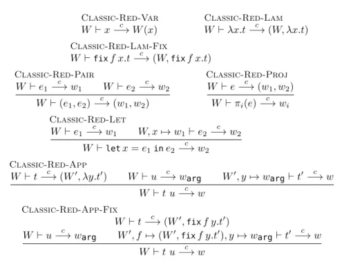
In this section, we will define an operational semantics for our term language, and use it to prove the soundness of the type system (Theorem 1). Our semantics is equivalent to the usual call-by-value big-step reduction semantics for the lambda-calculus in the sense that computation happens at the same time. There is however a notable difference.
Function closures are not built in the same way as they are in classical big-step semantics. Usually, we have a rule of the form V ⊢ λx.t −→ (V, λx.t) where
the closure for λx.t is a pair of the value environment V (possibly restricted to its subset appearing in t) and the function code. In contrast, we capture no values at closure creation time in our semantics: V ⊢ λx.t −→ (∅, λx.t). The captured values
will be added to the closure incrementally, during the reduction of binding forms that introduced them in the context.
Consider for example the following two derivations; one in the classic big-step reduction, and the other in our alternative system.
Classic-Red-Let
x:v⊢ x−→ vc x:v, y:v ⊢ λz.y−→ ((x 7→ v, y 7→ v), λz.y)c x:v⊢lety = xinλz.y−→ ((x 7→ v, y 7→ v), λz.y)c
Our-Red-Let
x:v⊢ x −→ v
x:v, y:v⊢ λz.y −→ ([x, y], ∅, λz.y) (∅, λz.y) y⇝ ([x], y 7→ v, λz.y)\v
x:v⊢lety = xinλz.y−→ ([x], y 7→ v, λz.y)
Rather than capturing the whole environment in a closure, we store none at all at the beginning (merely record their names), and add values incrementally, just before they get popped from the environment. This is done by the value substitution judgment w x⇝ w\v ′that we will define in this section. The reason for this choice is
that this closely corresponds to our typing rules, value substitution being a runtime counterpart to substitution in types Γ ⊢ σ x⇝ Γ\Φ ′ ⊢ σ′; this common structure is
essential to prove of the type soundness (Theorem 1).
Note that derivations in this modified system and in the original one are in one-to-one mapping. It should not be considered a new dynamic semantics, rather a reformulation that is convenient for our proofs as it mirrors our static judgment structure.
3.0.5 Values and Value Substitution
Values are defined as follows.
Val∋ v, w ::= values
| vα value of atomic type
| (v, w) value tuples
| ([xj]j∈J, (xi7→ vi)i∈I, λx.t) function closures
| ([xj]j∈J, (xi7→ vi)i∈I,fixf x.t) recursive function closures
The set of variables bound in a closure is split into an ordered mapping (xi7→
vi)i∈I for variables that have been substituted to their value, and a simple list
[xj]j∈J of variables whose value has not yet been captured. They are both binding
occurrences of variables bound in t; α-renaming them is correct as long as t is updated as well.
To formulate our type soundness result, we define a typing judgment on values Γ ⊢ v : σ in Figure 4. An intuition for the rule Value-Closure is the following.
Value-Atom Γ⊢ Γ⊢vα: α Value-Product Γ⊢ v1: τ1 Γ⊢ v2: τ2 Γ⊢ (v1, v2) : τ1∗ τ2 Value-Closure Γ, Γ1⊢ ∀i ∈ I, Γ, (xj:τj)j<i⊢ vi: τi ΓΦ, (xi:τiψi)i∈I, x:σϕ⊢ t : τ ΓΦ, (xi:τiψi)i∈I, x:σϕ⊢ τ (xi)\(Ψi) ⇝ ΓΦ′, x:σϕ ⊢ τ′ Γ, Γ1⊢ (dom(Γ), (xi7→ vi)i∈I, λx.t) : [ΓΦ ′ ](x:σϕ)→ τ′ Value-Closure-Fix Γ, Γ1⊢ ∀i ∈ I, Γ, (xj:τj)j<i⊢ vi: τi ΓΦ, (xi:τiψi)i∈I, f :([Γ, (xi:τiψi)](x:σ ϕ)→ τ)χ, x:σϕ⊢ t : τ ΓΦ, (xi:τiψi)i∈I, x:σϕ⊢ τ (xi)\(Ψi) ⇝ ΓΦ′, x:σϕ⊢ τ′
Γ, Γ1⊢ (dom(Γ), (xi7→ vi)i∈I,fixf x.t) : [ΓΦ
′
](x:σϕ)→ τ′ Figure 4: Value typing
Subst-Value-Atom vα y\v ⇝ vα Subst-Value-Product w1 y\v ⇝ w′ 1 w2 y\v ⇝ w′ 2 (w1, w2) y\v ⇝ (w′ 1, w2′) Subst-Value-Closure ([xj1, . . . , xjn, y], (xi7→ wi)i∈I, t) y\v ⇝ ([xj1, . . . , xjn], (y7→ v)(xi7→ wi)i, t) Subst-Value-Closure-Notin y /∈ (xj)j∈J ([xj]j∈J, (xi7→ wi)i∈I, t) y\v ⇝ ([xj]j∈J, (xi7→ wi)i∈I, t)
Figure 5: Value substitution
Internally, the term t has a dependency ΓΦon the ambient context, but also
depen-dencies (τψi
i ) on the captured variables. But externally, the type may not mention
the captured variables, so it reports a different dependency ΓΦ′ that corresponds to
the internal dependency ΓΦ, combined with the dependencies (Ψ
i) of the captured
values. Both families (ψi)i∈I and (Ψi)i∈I are existentially quantified in this rule.
In the judgment rule, the notation (xj: τj)j<iis meant to define the environment
of each (xi : τi) as ΓΦ, plus all the (xj : τj) that come before xi in the typing
judgment ΓΦ, (x
i : τi)i∈I, x : σϕ ⊢ t. The notation . . .
(xi)\(Ψi)
⇝ . . . denotes the
sequence of substitutions for all (xi, Ψi), with the rightmost variable (introduced
last) substituted first: in our dynamic semantics, values are captured by the closure in the LIFO order in which their binding variables enter and leave the lexical scope.
3.0.6 Substituting Values
In the typing rules, we use the substitution relation Γ, y:ρ⊢ σ y⇝ Γ ⊢ τ to\Φ remove the variable y from the closure types in σ. Correspondingly, in our runtime semantics, we add the variable y to the vector stored in the closure value, by a value substitution judgment w y⇝ w\v ′ (see Figure 5) when the binding of y is removed
from the evaluation context.
In theSubst-Value-Closure, the notation , (y7→ v)(xi 7→ wi)i means that the
binding y7→ v is added in first position in the vector of captured values. The values wi were computed in a context depending on y, so they need to appear after the
Lemma 4 (Value substitution preserves typing) If (Γ⊢ v : ρ), (Γ, y:ρ ⊢ w : σ), (Γ, y:ρ⊢ σ y⇝ Γ ⊢ τ) and (w\Ψ y⇝ w\v ′) hold, then (Γ⊢ w′ : τ ) holds.
Note that this theorem is restricted to substitutions of the rightmost variable of the context. While substitution in types needs to operate under binders (in rule Subst-Closure), value substitution is a runtime operation that will only be used by our (weak) reduction relation on the last introduced variable.
By induction on the value typing judgment Γ, y:ρ⊢ w : σ.
Case Value-Atom: by inversion we know that the last rule of Γ, y:ρ⊢ α y⇝ Γ ⊢ τ\Ψ is Subst-Atom. From the premise Γ, y:ρ ⊢ and Γ, y:ρ y⇝ Γ we can deduce\Ψ from Lemma1 that Γ⊢, which allows to conclude Γ ⊢vα: α.
Case Value-Product: by inversion, the last rules of Γ, y:ρ⊢ (σ1∗ σ2)
y\Ψ
⇝ Γ ⊢ τ and w y⇝ w\v ′ are respectively Subst-Product and Subst-Value-Product, so by induction hypothesis we have Γ⊢ w′1: τ1and Γ⊢ w2′ : τ2, which allows
us to conclude Γ⊢ (w′1, w′2) : τ1∗ τ2.
Case Value-Closure. By inversion we know that the last substitution rules applied are eitherSubst-ClosureandSubst-Value-Closure, orSubst-Closure-Notin andSubst-Value-Closure-Notin, depending on whether the substituted vari-able is part of the closure context.
In the latter case, both the types and the judgments are unchanged, so the result is immediate. If the substituted value is part of the closure context, the rules of the involved judgments are
Γ, y:ρ⊢ σ1 y\Ψ ⇝ Γ ⊢ σ1 Γ, y:ρ, x:σ1⊢ σ2 y\Ψ ⇝ Γ, x:σ1⊢ σ2′ Γ, y:ρ⊢ [ΓΦ1, y:ρχ](x:σϕ 1)→ σ2 y\Ψ ⇝ Γ ⊢ [ΓΦ1+χ.Ψ](x:σ 1ϕ)→ σ2′
∀i ∈ I, Γ, y:ρ, (xj:τj)j<i⊢ wi: τi ΓΦ
′′ 1, y:ρχ′′, (x i:τ ψi i )i∈I, x:σ1ϕ⊢ t : σ2′′ ΓΦ′′1, y:ρχ′′, (xi:τψi i )i∈I, x:σ1ϕ⊢ σ2′′ (xi)\(Ψi) ⇝ ΓΦ1, y:ρχ, x:σ 1ϕ ⊢ σ2
Γ, y:ρ⊢ (dom(Γ), (xi 7→ wi)i∈I, λx.t) : [ΓΦ1, y:ρχ](x:σ1ϕ)→ σ2
([dom(Γ), y], (xi7→ wi)i∈I, t) y\v
⇝ (dom(Γ), (y7→ v)(xi7→ wi)i, t)
We can reach our goal by using the following inference rule:
∀i ∈ I, Γ, y:ρ, (xj:τj)j<i⊢ wi: τi
ΓΦ′′1, y : ρχ′′, (xi:τiψi) i∈I, x:σ1ϕ ⊢ t : σ2′′ ΓΦ′′1, y:ρχ′′, (x i:τ ψi i )i∈I, x:σ1ϕ⊢ σ′′2 ,y(xi)i\,Ψ(Ψi)i ⇝ ΓΦ1+χ.Ψ, x:σ 1ϕ⊢ σ′2 Γ⊢ (dom(Γ), , (y7→ v)(xi 7→ wi)i∈I, λx.t) : [ΓΦ1+χ.Ψ](x:σ1ϕ)→ σ2′
The typing assumptions all match those of our premise. The reduction as-sumption is simply the composition of the reductions of the premises:
ΓΦ′′1, y:ρχ′′, (x i:τiψi)i∈I, x:σ1ϕ⊢ σ2′′ (xi)\(Ψi) ⇝ ΓΦ1, y:ρχ, x:σ 1ϕ⊢ σ2 y\Ψ ⇝ ΓΦ1+χ.Ψ, x:σ 1ϕ ⊢ σ2′
Red-Var
V ⊢ x −→ V (x)
Red-Lam
V ⊢ λx.t −→ (dom(V ),∅, λx.t)
Red-Lam-Fix
V ⊢fixf x.t−→ (dom(V ),∅,fixf x.t)
Red-Pair V ⊢ e1−→ v1 V ⊢ e2−→ v2 V ⊢ (e1, e2)−→ (v1, v2) Red-Proj V ⊢ e −→ (v1, v2) V ⊢ πi(e)−→ vi Red-Let V ⊢ e1−→ v1 V, (x7→ v1)⊢ e2−→ v2 v2 x\v1 ⇝ v′ 2 V ⊢letx = e1ine2−→ v′2 Red-App V, V1⊢ t −→ (dom(V ), V2, λy.t′) V, V1⊢ u −→ varg V, V1, V2, y7→ varg⊢ t′−→ w w y\varg ⇝ w′ V⇝ w2 ′′ V, V1⊢ t u −→ w′′ Red-App-Fix
V, V1⊢ t −→ (dom(V ), (xi7→ vi)i∈I,fixf y.t′)
V, V1⊢ u −→ varg V, (xi7→ vi)i, (f7→fixf y.t′), (y7→ varg)⊢ t′−→ w
V, V1⊢ t u −→ w
Figure 6: Big-step reduction rules
3.0.7 The Big-Step Reduction Relation
We are now equipped to define in Figure 6 the big-step reduction relation on well-typed terms V ⊢ e −→ v, where V is a mapping from the variables to values
that is assumed to contain at least all the free variables of e. The notation w V2
⇝ w′
denotes the sequence of substitutions for each (variable, value) pair in V2, from the
last one introduced in the context to the first; the intermediate values are unnamed and existentially quantified.
We write V : Γ⊢ if the context valuation V , mapping free variables to values, is well-typed according to the context Γ.
Value-Env-Empty
∅ : ∅ ⊢
Value-Env
V : Γ⊢ Γ⊢ v : σ
V, x7→ v : Γ, x:σ ⊢
Theorem 1 (Type soundness) If ΓΦ ⊢ t : σ, V : Γ ⊢ and V ⊢ t −→ v then
Γ⊢ v : σ.
By induction on the reduction derivation V ⊢ t −→ v. Case Red-Var: From V : Γ⊢ we have Γ ⊢ V (x) : σ.
Case Red-Lam,Red-Lam-Fix: in the degenerate case where there are no captured values, the value typing rule Value-Closure for [ΓΦ](x:σϕ)→ τ has as only
premise ΓΦ, x:σϕ⊢ τ, which is precisely our typing assumption.
Case Red-Let: The involved derivations are the following: V ⊢ e1−→ v1 V, x7→ v1⊢ e2−→ v2 v2 x\v1 ⇝ v′ 2 V ⊢letx = e1ine2−→ v′2 ΓΦdef⊢ e1: σ ΓΦbody, x:σϕ⊢ e2: τ Γ, x:σ⊢ τ x\Φdef ⇝ Γ ⊢ τ′
Γϕ.Φdef+Φbody⊢letx = e1ine2: τ′
By induction hypothesis we have Γ ⊢ v1 : σ, from which we deduce that
V, x 7→ v1 : Γ, x:σ ⊢. This allows us to use induction again to deduce that
Γ, x:σ ⊢ v2 : τ . Finally, preservation of value typing by value substitution
(Lemma4) allows to conclude that the remaining goal Γ⊢ v′
2: τ′ holds.
Case Red-App: the involved derivations are the following.
V, V1⊢ t −→ (dom(V ), (xi7→ vi)i∈I, λy.t′) V, V1⊢ u −→ varg
V, V1, (xi7→ vi)i, y7→ varg⊢ t′ −→ w w y\varg ⇝ w′ (xi)\(vi) ⇝ w′′ V, V1⊢ t u −→ w′′ (Γ, Γ1)Φfun⊢ t : [ΓΦclos](y:σϕ)→ τ (Γ, Γ1)Φarg⊢ u : σ Γ, y:σ⊢ τ y\Φarg ⇝ Γ ⊢ τ′
(Γ, Γ1)Φfun+Φclos+ϕ.Φarg⊢ t u : τ′
By induction we have that Γ, Γ1 ⊢ varg : σ and Γ ⊢ ((xi 7→ vi)i, λy.t′) :
[ΓΦclos](y:σϕ)→ τ.
By inversion, we know that the derivation for this value typing judgment is of the form
Γ, Γ1⊢ ∀i ∈ I, Γ, (xj:τj)j<i⊢ vi: τi ΓΦ, (xi:τiψi)i∈I, y:σϕ⊢ t′: τ′′
ΓΦ, (xi:τ ψi
i )i∈I, y:σϕ⊢ τ′′ (x
i)\(Ψi)
⇝ ΓΦclos, y:σϕ⊢ τ
Γ, Γ1⊢ (dom(Γ), (xi7→ vi)i∈I, λy.t′) : [Γ
Φ
clos](y:σϕ)→ τ
From our result Γ, Γ1⊢ vargand the premises Γ, (xj:τj)j<i⊢ vi: τiwe deduce
that the application valuation is well-typed with respect to the application environment: V, V1, (xi 7→ vi)i, y 7→ varg : Γ, Γ1, (xi:τi), σ ⊢. It is used in
the premise of the body computation judgment, so by induction we get that Γ, Γ1, (xi:τi), y:σ⊢ w : τ′′.
From there, we wish to use preservation of value typing on the chain of value substitutions wy\v⇝ warg ′ (xi)\(vi)
⇝ w′′ to conclude that Γ⊢ w′′: τ′. However,
the type substitutions of our premises are in the reverse order: ΓΦ, (xi:τiψi)i∈I, y:σϕ⊢ τ′′ (x i)\(Ψi) ⇝ ΓΦclos, y:σϕ ⊢ τ y\Φarg ⇝ ΓΦ clos+ϕ.Φarg⊢ τ′ we therefore need to use our Reordering Lemma (1) to get them in the right order — note that the annotations (Ψi)i∈I and Φargare not changed as they are independent from each other: for any i, we have Ψi(y) = Φarg(xi) = 0.
ΓΦ, (xi:τ ψi i )i∈I, y:σϕ⊢ τ′′ y\Φarg ⇝ ΓΦ′ clos, (xi:τ ψi i )i∈I ⊢ τ (xi)\(Ψi) ⇝ ΓΦclos+ϕ.Φarg⊢ τ′ Finally, we recall the usual big-step semantics for the call-by-value calculus with
Classic-Red-Var W ⊢ x−→ W (x)c Classic-Red-Lam W ⊢ λx.t−→ (W, λx.t)c Classic-Red-Lam-Fix W ⊢fixf x.t−→ (W,c fixf x.t) Classic-Red-Pair W ⊢ e1 c −→ w1 W ⊢ e2 c −→ w2 W ⊢ (e1, e2) c −→ (w1, w2) Classic-Red-Proj W ⊢ e−→ (wc 1, w2) W ⊢ πi(e) c −→ wi Classic-Red-Let W ⊢ e1 c −→ w1 W, x7→ w1⊢ e2 c −→ w2 W ⊢letx = e1ine2 c −→ w2 Classic-Red-App
W ⊢ t−→ (Wc ′, λy.t′) W ⊢ u−→ wc arg W′, y7→ warg⊢ t′ −→ wc W ⊢ t u−→ wc
Classic-Red-App-Fix
W ⊢ t−→ (Wc ′,fixf y.t′)
W ⊢ u−→ wc arg W′, f 7→ (W′,fixf y.t′), y7→ warg⊢ t′−→ wc
W ⊢ t u−→ wc
Figure 7: Classic big-step reduction rules
Due to space restriction we will only mention the rules that differ, and elide the equivalence proof, but the long version contains all the details.
There is a close correspondence between judgments of both semantics, but as the value differ slightly, in the general cases the value bindings of the environment will also differ. We state the theorem only for closed terms, but the proof will proceed by induction on a stronger induction hypothesis using an equivalence between non-empty contexts.
Theorem 2 (Semantic equivalence) Our reduction relation is equivalent with
the classic one on closed terms: ∅ ⊢ t −→ v holds if and only if ∅ ⊢ t c
−→ v also holds.
To formulate our induction hypothesis, we define the equivalence judgment V ⊢ v = W
c
⊢ w; on each side of the equal sign there is a context and a value, the
right-hand side being considered in the classical semantics.
∅ ⊢ = ∅⊢c V ⊢ = W c ⊢ V ⊢ v = W c ⊢ w V, x7→ v ⊢ = W, x 7→ w c ⊢ V ⊢ = W c ⊢ V ⊢vα= W c ⊢vα V ⊢ v1= W c ⊢ w1 V ⊢ v2= W c ⊢ w2 V ⊢ (v1, v2) = W c ⊢ (w1, w2) V ⊢ = W c ⊢ V, xi 7→ vi⊢ = W′ c ⊢ V ⊢ ((xi 7→ vi)i∈I, λx.t) = W c ⊢ (W′, λx.t)
The stronger version of the theorem becomes the following: if V ⊢ = W ⊢ andc V ⊢ t −→ v and W ⊢ t−→ w, then V ⊢ v = Wc
c
As for subject reduction, we first need to prove that value substitution preserves value equivalence.
Lemma 5 (Value substitution preserves value equivalence) If V, y 7→ v0 ⊢
v = W c ⊢ w, V ⊢ v0= W c ⊢ w0, and v y\v0 ⇝ v′ then V ⊢ v′= W ⊢ w.c
Case Subst-Value-Atom: direct.
Case Subst-Value-Product: direct induction.
Case Subst-Value-Closure: We have ((xi 7→ vi)i∈I, λx.t) y\v0
⇝ (, y 7→ v0(xi 7→
vi)i∈I, λx.t) and V, y 7→ v0 ⊢ ((xi 7→ vi)i∈I, λx.t) = W ⊢ (W′, λx.t). The
latter implies V, y7→ v0, xi7→ vi ⊢ = W′ c
⊢ which which in turn implies our
goal V ⊢ (, y 7→ v0) – with the additional premise V ⊢ = W
c
⊢ from our
hypothesis V ⊢ v0= W
c
⊢ w0.
We can now prove the theorem proper:
Case Red-Var, Classic-Red-Var: we check by direct induction on the contexts that if V ⊢ = W ⊢ holds, then V ⊢ V (x) = Wc ⊢ W (x).c
Case Red-Lam,Classic-Red-Lam: The correspondence between V ⊢ (∅, λx.t) and W
c
⊢ (W, λx.t) under assumption V ⊢ = W ⊢ is direct from the inferencec
rule V,∅ ⊢ = W c ⊢ V ⊢ (∅, λx.t) = W c ⊢ (W, λx.t)
Case Red-Pair, Classic-Red-Pair and Red-Proj, Classic-Red-Proj: direct by induction.
Case Red-Let,Classic-Red-Let: By induction hypothesis on the e1 premise, we
deduce that V ⊢ v1 = W
c
⊢ w1, hence V, x 7→ v1 ⊢ = W, x 7→ w1
c
⊢ . This
lets us deduce, again by induction hypothesis, that V, x7→ v1⊢ v2= W, x7→
w1
c
⊢ w2. As value substitution preserves value equivalence, we can deduce
from v2
x\v1
⇝ v′
2 that our goal V ⊢ v2′ = W
c
⊢ w2 holds.
Case Red-App, Classic-Red-App: By induction hypothesis we have that V ⊢ varg = W ⊢ warg and V ⊢ ((xi 7→ vi)i∈I, λy.t′) = W
c
⊢ (W′, λy.t′). By
inversion on the value equivalence judgment of the latter we know that V, xi7→
vi ⊢ = W′ c
⊢ . Combined with the former value equivalence, this gives us V, xi 7→ vi, y 7→ varg⊢ = W′, y 7→ warg
c
⊢ , so by induction hypothesis and
preservation of value equivalence by reduction we can deduce our goal.
4
Dependency information as non-interference
We can formulate our dependency information as a non-interference property. Two valuations V and V′ are Φ-equivalent, noted V =ΦV′, if they agree on all
vari-ables on which they depend according to Φ. We say that e respects non-interference for Φ when, whenever V ⊢ e −→ v holds, then for any V′ such that V =Φ V′ we
have that V′ ⊢ e −→ v also holds. This corresponds to the information-flow
se-curity idea that variables marked 1 are low-sese-curity, while variables marked 0 are high-security and should not influence the output result.
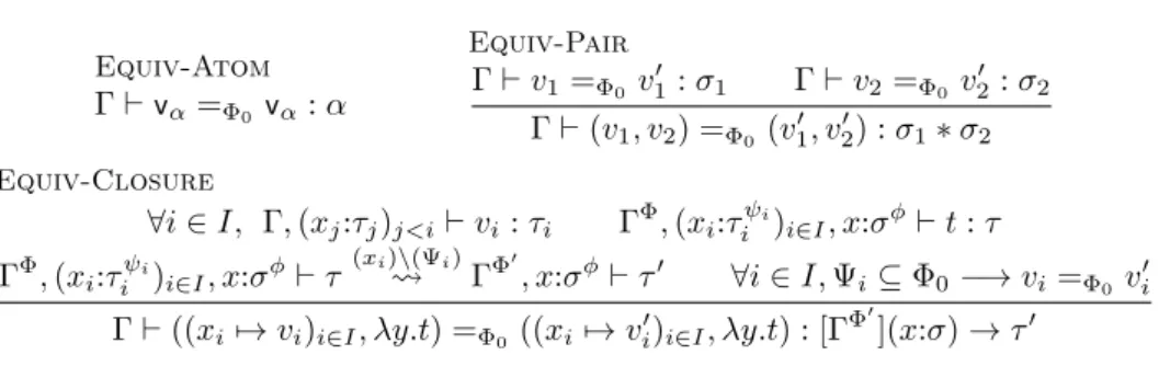
Equiv-Atom Γ⊢vα=Φ0 vα: α Equiv-Pair Γ⊢ v1=Φ0 v ′ 1: σ1 Γ⊢ v2=Φ0v ′ 2: σ2 Γ⊢ (v1, v2) =Φ0 (v ′ 1, v′2) : σ1∗ σ2 Equiv-Closure
∀i ∈ I, Γ, (xj:τj)j<i⊢ vi: τi ΓΦ, (xi:τiψi)i∈I, x:σϕ⊢ t : τ
ΓΦ, (xi:τ ψi i )i∈I, x:σϕ⊢ τ (xi)\(Ψi) ⇝ ΓΦ′, x:σϕ⊢ τ′ ∀i ∈ I, Ψi ⊆ Φ0−→ vi =Φ0v′i Γ⊢ ((xi7→ vi)i∈I, λy.t) =Φ0 ((xi7→ v ′ i)i∈I, λy.t) : [ΓΦ ′ ](x:σ)→ τ′ Figure 8: Value equivalence
This non-interference statement requires that the two evaluations of e return the same value v. This raises the question of what is the right notion of equality on values. Values of atomic types have a well-defined equality, but picking the right notion of equality for function types is more difficult. While we can state a non-interference result on atomic values only, the inductive subcases would need to handle higher-order cases as well.
Syntactic equality (even modulo α-equivalence) is not the right notion of equal-ity for closure values. Consider the following example: x:τ0 ⊢ lety = xinλz.z :
[x:τ0](z : σ1) → σ. This term contains an occurrence of the variable x, but its
result does not depend on it. However, evaluating it under two different contexts
x:v and x:v′, with v ̸= v′, returns distinct closures: (x 7→ v, λz.z) on one hand,
and (x 7→ v′, λz.z) on the other. These closures are not structurally equal, but
their difference is not essential since they are indistinguishable in any context. Log-ical relations are the common technique to ignore those internal differences and get a more observational equality on functional values. They involve, however, a fair amount of metatheoretical effort (in particular in presence of non-terminating fixpoints) that we would like to avoid.
Consider a different example: x:τ0 ⊢ λy.x : [x:τ1](y:σ0)→ τ. Again, we could
use two contexts x:v and x:v′with v̸= v′, and we would get as a result two closures:
x:v ⊢ λy.x −→ (x 7→ v, λy.x) and x:v′ ⊢ λy.x −→ (x 7→ v′, λy.x). Interestingly,
these two closures are not equivalent under all contexts: any context applying the function will be able to observe the different results. However, our notion of interference requires that they can be considered equal. This is motivated by real-world programming languages that only output a pointer to a closure in a program that returns a function.
While the aforementioned closures are not equal in any context, they are in fact equivalent from the point of view of the particular dependency annotation for which we study non-interference, namely x:τ0. To observe the difference between those
closures, we would need to apply the closure of type [x:τ1](y : σ)→ τ, so would be
in the different context x:τ1.
This insight leads us to our formulation of value equivalence in Figure8. Instead of being as modular and general as a logical-relation definition, we fix a global
dependency Φ0 that restricts which terms can be used to differentiate values.
Our notion of value equivalence, Γ⊢ v =Φ0 v′ : σ is typed and includes structural
equality. In the ruleEquiv-Closure, we check that the two closures values are well-typed, and only compare captured values whose dependencies are included in those of the global context Φ0, as we know that the others will not be used. This equality
is tailored to the need of the non-interference result, which only compares values resulting from the evaluation of the same subterm – in distinct contexts.
Theorem 3 (Non-interference) If ΓΦ0 ⊢ e : σ holds, then for any contexts V, V′
such that V =Φ0 V′ and values v, v′ such that V ⊢ e −→ v and V′ ⊢ e −→ v′, we
We will proceed by simultaneous induction on the typing derivation Γ ⊢ e : σ
and reduction derivation V ⊢ e −→ v and . Note that we use a different induction
hypothesis: for any subderivations ΓΦ⊢ e : σ and V ⊢ t −→ v, we will prove that
for any V′ that agrees with V on Φ modulo Φ0-equivalence (∀x, V (x) =Φ0 V′(x),
which we still note V =ΦV′), and with V′⊢ t −→ v′, we have v =Φ0 v′.
We will omit the contexts and types Γ, σ of a value equivalence Γ⊢ v =Φ0 v′: σ
when they are clear from the context.
Case Red-Var: from V =0,x:1,0V′ we have V (x) =Φ0V′(x).
Case Red-Lam, Red-Lam-Fix : the returned value does not depend on the envi-ronment.
Case Red-Pair,Red-Proj: direct by induction.
Case Red-Let: the involved derivations are the form
ΓΦdef⊢ e1: σ ΓΦbody, x:σϕ⊢ e2: τ
ΓΦbody+ϕ.Φdef⊢letx = e1ine2: τ
V ⊢ e1−→ v1 V, x7→ v1⊢ e2−→ v2 v2 x\v1 ⇝ v3 V ⊢letx = e1ine2−→ v3 V′ ⊢ e1−→ v1′ V′, x7→ v′1⊢ e2−→ v2′ v2′ x\v1′ ⇝ v′ 3 V′⊢letx = e1ine2−→ v′3
The context equivalence V =Φbody+ϕ.ΦdefV′ implies the weaker equivalence
V =Φ
body V′, from which we can deduce V, x 7→ v1 =(Φbody,ϕ) V
′, x 7→ v′
1
regardless of the value of ϕ. Indeed, if ϕ is 0 this is direct, and if ϕ is 1 we get
v1 =Φ0 v1′ by induction hypothesis. From this equality between contexts we
get v2=Φ0 v′2 by induction hypothesis.
We then reason by case distinction on the property Φdef⊆ Φ0. If it holds,
then again v1 =Φ0 v1′ by induction, so substituting v1, v′1 in the closures of
v2, v′2 will preserve Φ0-equivalence. And if it does not, those values v1, v′1
captured in the closures of v2, v2′ will not be tested for Φ0-equivalence. In any
case, we have v3=Φ0 v3′.
Case Red-App: the proof for the application case uses the same mechanisms as for theRed-Letcase but is more tedious because of the repeated application and substitution of the closed-over values. To simplify notations, we will handle the case of a single captured value x7→ v. The involved derivations are the