Encoding and Decoding Neuronal Dynamics: Methodological Framework to Uncover the Algorithms of Cognition

(1)

HAL Id: hal-01848442

https://hal.archives-ouvertes.fr/hal-01848442

Preprint submitted on 24 Jul 2018

HAL is a multi-disciplinary open access archive for the deposit and dissemination of sci-entific research documents, whether they are pub-lished or not. The documents may come from teaching and research institutions in France or abroad, or from public or private research centers.

L’archive ouverte pluridisciplinaire HAL, est destinée au dépôt et à la diffusion de documents scientifiques de niveau recherche, publiés ou non, émanant des établissements d’enseignement et de recherche français ou étrangers, des laboratoires publics ou privés.

Encoding and Decoding Neuronal Dynamics:

Methodological Framework to Uncover the Algorithms

of Cognition

Jean-Rémi King, Laura Gwilliams, Chris Holdgraf, Jona Sassenhagen,

Alexandre Barachant, Denis Engemann, Eric Larson, Alexandre Gramfort

To cite this version:

Jean-Rémi King, Laura Gwilliams, Chris Holdgraf, Jona Sassenhagen, Alexandre Barachant, et al.. Encoding and Decoding Neuronal Dynamics: Methodological Framework to Uncover the Algorithms of Cognition. 2018. �hal-01848442�

(2)

Encoding and Decoding Neuronal

Dynamics: Methodological Framework to

Uncover the Algorithms of Cognition

King, J-R.1-2_{, Gwilliams, L.}1,3_{, Holdgraf, C.}4_{, Sassenhagen, J.}5_{, Barachant, A.}6_{, Engemann, D.}7_,

Larson, E.8_{, Gramfort, A}7,9_.

1. Psychology Department, New York University, New York, USA; 2. Frankfurt Institute for Advanced Studies, Frankfurt, Germany; 3. NYUAD Institute, Abu Dhabi, UAE; 4. Berkeley Institute for Data Science, Helen Wills Neuroscience Institute, UC Berkeley, USA; 5. Department of Psychology, Goethe-University Frankfurt, Frankfurt, Germany; 6. CTRL-labs, New York, USA;

7. Parietal Team, INRIA, CEA, Université Paris-Saclay, Gif-sur-Yvette, France; 8. Institute for Learning and Brain Sciences, University of Washington, Seattle, WA; 9. Laboratoire Traitement

et Communication de l'Information, INRIA Saclay, France

Abstract

A central challenge to cognitive neuroscience consists in decomposing complex brain signals into an interpretable sequence of operations - an algorithm - which ultimately accounts for intelligent behaviors. Over the past decades, a variety of analytical tools have been developed to (i) isolate each algorithmic step and (ii) track their ordering from neuronal activity. In the present chapter, we briefly review the main methods to encode and decode temporally-resolved neural recordings, show how these approaches relate to one-another, and summarize their main premises and challenges. Finally we highlight, through a series of recent findings, the increasing role of machine learning both as i) a method to extract convoluted patterns of neural activity, and as ii) an operational framework to formalize the computational bases of cognition. Overall, we discuss how modern analyses of neural time series can identify the algorithmic organization of cognition.

(3)

Introduction

An algorithm is a sequence of simple computations that can be followed to solve a complex problem. Under this definition, a major goal of cognitive neuroscience thus consists in uncovering the algorithm of the mind: i.e. identifying the nature and the order of computations implemented in the brain to adequately interact with the environment _{(Marr, 1982).}

Over the years, this foundational endeavor has adopted a variety of methods, spanning from the decomposition of reaction times _{(Donders, 1969; Sternberg, 1998) to the modern} electrophysiology and neuroimaging paradigms. In the present chapter, we focus on two major pillars necessary to recover an interpretable sequence of operations from neuronal activity. First, we review how individual computations can be isolated by identifying and linking neural codes to mental representations. Second, we review how the analysis of dynamic neural responses can recover the order of these computations. Throughout, we discuss how the recent developments in machine learning not only offer complementary methods to analyze convoluted patterns of neural activity, but also provide a formal framework to identify the computational foundations of cognition.

Figure 1. The representational paradigm. _{Cognitive neuroscience faces a triple challenge: it} aims to (i) identify the content of mental representations, (ii) determine how this information is encoded in the brain, and (iii) link these two levels of description. In the past decades, linking neural codes to mental representations has increasingly benefitted from statistical modeling and machine learning. In this view, decoding predicts experimental factors (e.g. the speed of a hand movement, the luminance of an flashed image etc) from specific features of brain activity (e.g. spike rate, electric field etc), whereas encoding predicts the reverse. Currently, the neural codes and the mental representations are engineered manually and linearly mapped onto one another with linear modeling. However, the capacity of machine learning to find non-linear structures in large datasets may ultimately help us find what the brain representations and how.

(4)

1. Neuronal activity: codes and contents.

1.1 The triple-quest of cognitive neuroscience.

Three challenges must be addressed to isolate the elementary computations underlying intelligent behavior (Fig. 1). First, we must identify what content the brain represents at each instant. For example, speech has been formally described in terms of phonemes (e.g. /b/, /p/, /k/). However, the psychological reality of these units has been debated given their extensive overlap with low-level acoustic properties. To address this issue, Mesgarani et al. have shown that responses in superior temporal gyrus to speech are more closely organized along phonetic dimensions than acoustic dimensions _{(Mesgarani, Cheung, Johnson, & Chang, 2014) (see (Di} Liberto, Di Liberto, O’Sullivan, & Lalor, 2015) for similar results with electro-encephalography - EEG). More generally, the search for mental representations is ubiquitous across the fields of cognitive neuroscience, and has helped to characterize the neural bases of faces _{(Freiwald &} Tsao, 2010; Haxby, 2006; Kanwisher, 2001)_{, word strings ((Dehaene & Cohen, 2007; Price,} 2010)_{, semantics (Huth, de Heer, Griffiths, Theunissen, & Gallant, 2016), to name a few.}

Second, we must identify _{how neurons read and communicate such informational} content. For example, the relative unreliability of neurons to discharge at precise moments has led some to argue that neurons transmit information through the rate at which they fire over a small temporal window _{(Shadlen & Newsome, 1998). By contrast, the speed of cognitive} processes, which can be as low as a few dozen milliseconds have led others to argue that rate-coding is unlikely to be the only neural code _{(Kistler & Gerstner, 2002). More generally,} whether neurons and neural populations code information via their firing rates _{(Shadlen &} Newsome, 1998)_{, their oscillatory activity (Buzsaki, 2006; Fries, 2005; Singer & Gray, 1995), or} even in the interaction between spikes and the phase of local field potentials _{(Bose & Recce,} 2001; Lisman & Idiart, 1995)_{remains actively debated.}

Historically, the dual challenge between _{what is being coded and how it is coded has} been approached through a univariate mapping between neural activity and mental contents. In this view, the objective consists of finding a neural response (e.g. a spike) that is both sensitive and specific to particular content (e.g. the orientation of a visual bar _{(Hubel & Wiesel, 1963)). To} facilitate this quest, it is now common to perform multivariate mapping. For example, one can assume a rate coding and test whether a neuron codes for a particular retinotopic location by simultaneously stimulating multiple sections of the visual field, and _{a posteriori modeling the} independent contribution of each location _{(Wandell, Dumoulin, & Brewer, 2007). Reciprocally,} one can assume that neurons code for retinotopic locations and test whether this information can be better decoded from rate than from temporal coding _{(Nishimoto et al., 2011). In all} analyses, there thus exists an asymmetry in the code-representation equation: either the type of neural code is assumed and multiple representations are estimated, or _{vice versa}. This asymmetry has contributed to the distinction between encoding and decoding analyses. Specifically, encoding consists in predicting neuronal responses from mental representations:

(5)

(P(brain activity | representations)). Conversely, decoding consists in predicting mental representations from neuronal activity (P(representations | brain activity)) (See Fig 1.).

Figure 2. Statistical framework. Left. _{The modeling of neural representations is founded on} a general statistical framework. _{Middle. Models can be distinguished across three main} dimensions. First, models that are optimized to estimate the conditional probability P(Y|X) are ‘discriminative’, whereas models that estimate the joint distribution (P(X,Y)) are ‘generative’ (All generative models can thus be discriminative). Second, models trained to predict one variable X from another Y are ‘supervised’, whereas models that estimate the distribution of a single (possibly multidimensional) variable are ‘unsupervised’. Finally, a given model can be used for different purposes: e.g. decoding or encoding. _{Right. Example of classical} supervised and unsupervised models.

Encoding analyses have been predominantly used to simultaneously examine several features in their ability to account for univariate brain responses. For example, the general linear model (GLM) routinely used in fMRI studies is designed to evaluate the extent to which multiple features independently contribute the blood-oxygen-level dependent (BOLD) response recorded in each voxel. Such effects can be hard to orthogonalize _{a priori} (i) because of the slow temporal profile of the hemodynamic response or (ii) because the features under investigation intrinsically covary (e.g. in natural images, the orientation of visual edges correlate with their spatial position _{(Sigman, Cecchi, Gilbert, & Magnasco, 2001)). Conversely, decoding analyses} have been predominantly used to predict subjects’ behavior or postdict their sensory stimulations. For example, brain-computer interfaces (BCI) focus on simultaneously examining several, potentially collinear patterns of brain activity to predict subjects’ actions, intentions (Lebedev & Nicolelis, 2006)_{or mental state (Zander & Kothe, 2011).}

(6)

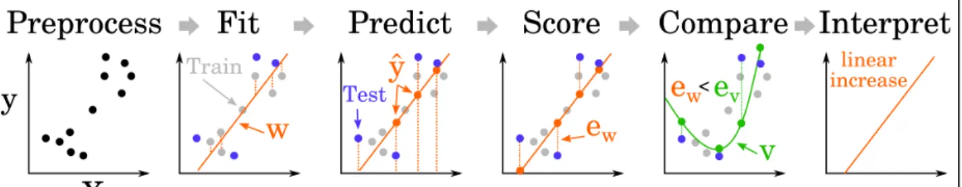
Figure 3. Modeling pipeline. _{Multivariate analyses aim to identify the combination of} parameters (w) that maximize the relationship between neural codes and mental representations. The potentially large number of fitted parameters rapidly leads to overfitting - i.e. to identifying an overly complex relationship in the data sample that poorly generalizes to the general population. To prevent overfitting, a standard multi-step pipeline must be adopted. It starts with 1) preprocessing (any transformation of the data that can be applied independently of the overall sample: e.g. filtering), followed by 2) model fitting on a subset of the data (a.k.a ‘training set’, in gray), 3) prediction (orange dots) of independent and identically distributed (iid, see_{(Varoquaux et al., 2017) for guidelines) held out test data (blue} dots) and 4) summarizing the prediction errors of the model (e) with a scoring metrics (e.g. Accuracy, AUC, R2_{, cross-entropy etc). In addition, one can subsequently perform 4) model}

comparison and/or 5) interpret the parameters of the model see _{(Haufe et al., 2014) for} guidelines). The score of a model (e.g. goodness of fit, accuracy) is often easier to interpret than its numerous parameters because of two reasons. First, the score of a model reduces multiple, potentially noisy, dimensions to a low-dimensional, often singleton, quantity. Second, the model parameters are generally optimized for predictive performance but do not necessarily constitute a unique solution to a given problem.

1.2 Where do the linearity assumptions come from?

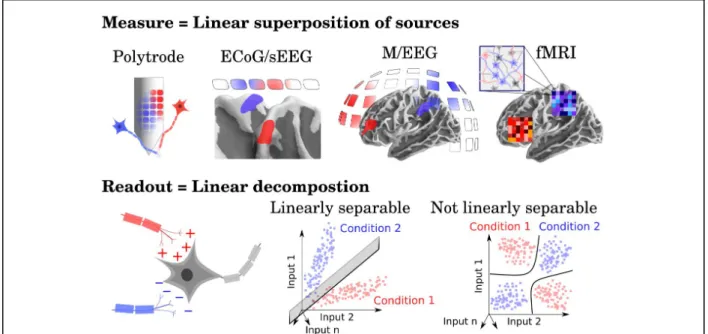
Encoding and decoding analyses of brain activity are predominantly based on linear modeling. The linear constraint is motivated by two theoretical principles: i) the linear superposition principle, and ii) the linear readout principle (Fig. 4).

Linear superposition is a common assumption based on the notion that measurements are derived from a weighted sum of independent sources. For example, the electric potential measured by an electrode depends on the electric reference, the local field potential, as well as on the pre and postsynaptic activity of surrounding neurons. Following Maxwell’s equations, the electric fields of these sources linearly sum onto the electrode, and do not interact with one another. The analysis of hemodynamic responses is often based on an analogous measurement assumption: each voxel contains hundreds of thousands of neurons whose activity is summarized in a unique BOLD measurement. Under the linear superposition assumption, a measurement linearly covaries with a variable only if a combination of sources linearly covaries with such variables. It is possible to separate the independent contribution of each source when multivariate measurements are available, based on physical assumptions (as in MEG source reconstruction_{(Hämäläinen, Hari, Ilmoniemi, Knuutila, & Lounasmaa, 1993)), or} based on distributional assumptions (as in spike sorting _{(Quiroga, Nadasdy, & Ben-Shaul,} 2004)_{). Note that the linear superposition assumption is generally limited to a specific range. For}

(7)

example, the BOLD response is known to saturate above certain values, above which the linear superposition assumption breaks _{(Heeger & Ress, 2002).}

The linear readout principle is specific to neuroscience, and is based on the notion that the function of neurons and neural assemblies can be approximated with a non-linear transformation (e.g. a spike) of a weighted sum of electrico-chemical input (e.g. the sum of excitatory and inhibitory presynaptic potentials). This computational constraint can thus be used to formalize several definitions. First a feature is considered to be explicitly represented if and only if it is linearly readable in the brain activity _{(Hung, Kreiman, Poggio, & DiCarlo, 2005;} Kamitani & Tong, 2005; King & Dehaene, 2014; Kriegeskorte & Kievit, 2013; Misaki, Kim, Bandettini, & Kriegeskorte, 2010)_{. Second, a representation, which characterizes the} relationships between these features, is defined by a set of basis vectors. In this view, the retina may encode _{information about faces, strings and objects, but would not represent these} categories, in that faces, string and objects cannot be linearly separated from retinal activations.

Figure 4. _{Motivating the linear assumptions. Linear models are not only popular because} of their efficiency and simplicity, but also because they rely on two theoretically-motivated assumptions. First, neuroscientific measurements involve the superposition of multiple responses at all scales (e.g. dendritic, neuronal and network). The linear superposition principle is an _{epistemic assumption that helps cognitive neuroscientists to isolate the coding} contribution of each of these sources. Second, the linear readout principle is a _{computational} assumption and consists in defining representation as linearly separable information. The linear readout principle is motivated by the notion that the response function of individual neurons as well as neuronal populations can be reasonably approximated as a linear sum of excitatory and inhibitory presynaptic potentials followed by a (series of) spikes (i.e. applying a non-linear operation onto a weighted sum).

(8)

Under these definitions, encoding and decoding analyses are equally limited in their ability to determine whether a representation _{de facto constitutes information that the neural} system _uses. For example, one may find a linear relationship between a sensory feature and (i) a spike, (ii) an increase in BOLD response, or (iii) an oscillation of a linear combination of EEG sensors, without that information being effectively read and used by any neurons. Similarly to all other correlational methods, encoding and decoding must thus be used in conjunction with computational modeling and experimental manipulations in order to identify the causal or epiphenomenal nature of an identified pattern of brain activity.

1.3 Challenging the representational paradigm.

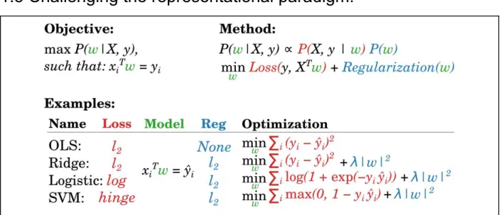
Figure 5. _{A zoo of linear models? While linear models are ubiquitous in cognitive} neuroscience, their many designations can be formalized as finding a set of weights (w) that can be used in combination to predict values (y) from multivariate data (X). The method equations shows that such estimation of w can be done by so-called maximum a posteriori (MAP), balancing the data likelihood (red) and the priors on the distribution of these parameters (blue). In an optimization framework, this transcribes into jointly minimizing the loss and regularization function. Note that for categorical models (e.g. Logistic regression, support vector classifier (SVM)), the predicted values ŷ are subsequently transformed into discrete categories.

A large number of multivariate analyses are routinely used in cognitive neuroscience, and range from linear discriminant analysis (LDA) to ridge and logistic regressions and linear support vector machines (SVM). Despite their various denominations, these analyses actually fit in a common statistical framework, and can be solved with similar optimization procedures (Fig. 5). In practice, these analyses make distinct assumptions on the data but often lead to similar results _{(Hastie, Tibshirani, & Friedman, 2009; Lebedev & Nicolelis, 2006) (Varoquaux et al.,} 2017)_.

(9)

The linearity constraint, present in most encoding and decoding analyses, entails two major challenges to the neuroscientific study of mental representations. First, the linear readout assumption undermines the non-linear readout abilities of neurons _{(Brincat & Connor, 2004;} Chichilnisky, 2001; Mineault, Khawaja, Butts, & Pack, 2012; Sahani & Linden, 2003; Van Steveninck & Bialek, 1988) _{, cortical columns (Bastos et al., 2012) and large neural assemblies} (Ritchie, Brendan Ritchie, Kaplan, & Klein, 2017) _{. We can thus expect that representations will} eventually be defined, not as set of basis-vectors but as non-linear manifolds _{(Jazayeri & Afraz,} 2017)_.

Second, linear modeling implies a strong dependence on _{a priori} human insight (Kording, Benjamin, Farhoodi, & Glaser, 2018) _{. Specifically, linear models only fit the features} explicitly provided by the experimenter. They are thus limited in their ability to identify unexpected patterns of neuronal activity, or unanticipated mental representations. For example, the discovery of grid cells - hippocampal neurons that fire when an animal is located at regularly-interspaced locations in an arena - strongly derived from human insight. Indeed, Moser et al. had to eyeball their electrophysiological data to conjecture the grid coding scheme _(Fyhn, Molden, Witter, Moser, & Moser, 2004; Moser, Kropff, & Moser, 2008) _{. Only then could they} input a grid feature in their linear model to test for its robustness _{(Hafting, Fyhn, Molden, Moser,} & Moser, 2005)_{. For this historical discovery, a linear model blindly fitting spiking activity to a} two-dimensional spatial position variable would have completely missed the grid coding scheme.

The rapid development of machine learning may partially roll back this epistemic dependence on human insights. For example, Benjamin and collaborators have recently investigated the ability of linear models to predict spiking activity in the macaque motor cortex given conventional representations of the arm movement, such as its instantaneous velocity and acceleration _{(Benjamin et al., 2017). The authors show that while linear encoding models for} these motor features accurately predict neural responses, they are outperformed by random forests _{(Liaw, Wiener, & Others, 2002) and long short term memory neural networks (LSTM} (Hochreiter & Schmidhuber, 1997) _{). Random forests and LSTMs are distinct non-linear models} commonly used in machine learning precisely because they are capable of modeling near-arbitrary functions from the data. In other words, machine learning algorithms can identify features in the arm movements that improve the prediction of neural activity. These results thus suggest that the spiking activity in the motor cortices encodes something beyond what was previously hypothesized. More generally, this study illustrates how machine learning may supplement human insights and help to discover unanticipated representations.

Undoubtedly, such machine-learning approaches to neuroscience will be accompanied with new challenges_{(Kording et al., 2018; Stevenson & Kording, 2011). In particular, non-linear} models remain currently difficult to inspect and interpret _{(Olah et al., 2018). For example, in} Benjamin et al’s study discussed above, the improvement of prediction _{performance provided by} machine learning algorithms came at the price of a diminished interpretability. Specifically, the authors have only shown that the brain represents more than the classic sensory-motor features, but have not revealed what these unsuspected representations actually corresponded to. Although such interpretability issue is particularly strong in non-linear modeling, it exists in linear modeling too. For example _{(Huth et al., 2016) used linear modeling to predict the fMRI}

(10)

BOLD responses to spoken stories from very large vectors describing the semantic values of each of the spoken words. The authors showed that this modeling approach was above chance level in a wide variety of cortical regions. To subsequently investigate what each brain region specifically represented, the authors used unsupervised linear model: principal component analysis (PCA). PCA summarized the main dimensions that accounted for the BOLD responses to semantic vectors. However, the authors only managed to make sense of a small subset of these principal dimensions. This study thus illustrates that robust linear modeling does not necessarily entail a straightforward interpretation.

2. From individual computations to algorithms.

The above methods isolate individual computations by linking mental representations with their neural implementations. However, to uncover the _{algorithm of a given cognitive ability,} one must also identify the order in which these computations are performed. Before quickly reviewing the analytical methods developed to track sequences of computations from brain activity, it is important to first highlight the prevalence of temporal structures in neuroimaging and electrophysiology recordings.

2.1 Sequences of neural responses.

With the recent advances in temporally-resolved fMRI _{(e.g. Ekman, Kok, & de Lange,} 2017) and the increasing ability to simultaneously record multiple neurons _{(Jun et al., 2017) and} brain regions _{(Boto et al., 2018; Tybrandt et al., 2018), numerous studies have evidenced} spatio-temporal structures in neural activity. For example, at the network level, sensory stimulations trigger a long cascade of neural responses from the sensory to associative cortices (e.g. _{(Gramfort, Papadopoulo, Baillet, & Clerc, 2011; King et al., 2016), Fig. 6.C). At the} columnar level, oscillatory activity propagates from and to the supra- and infragranular layers of the cortex through frequency-specific travelling waves _{(van Kerkoerle et al., 2014) (Fig. 6.B). At} the cellular level, spatial positions _{(Girardeau & Zugaro, 2011; Jones & Wilson, 2005), motor} preparation _{(Kao et al., 2015) and working memory processes (Heeger & Mackey, 2018;} Stokes, 2015) are associated with specific sequences of neuronal responses (Fig. 6.A). Finally, sequences of pre-synaptic inputs have recently been shown to be detectable by the dendrites of single neurons _{(Branco, Clark, & Häusser, 2010).}

These electrophysiological sequences are increasingly linked to specific sequences of computations - and thus proto-algorithms. For example, the sequential reactivation of hippocampal place cells is believed to reflect learning and anticipatory simulation of the spatial navigation _{(Girardeau & Zugaro, 2011) (Fig. 6.A). Analogously, the propagation of} frequency-specific traveling waves across the cortical microcircuit has been proposed to reflect a predictive coding algorithm_{(Bastos et al., 2012). Finally, the macroscopic sequence of brain} responses identified across brain regions can be directly compared to the deep convolutional networks built in artificial vision _{(Cichy, Khosla, Pantazis, Torralba, & Oliva, 2016; Eickenberg,}

(11)

Gramfort, Varoquaux, & Thirion, 2017; Gwilliams & King, 2017; Kriegeskorte, 2015; Yamins et al., 2014)_.

Figure 6. Sequences of neural responses across all spatial scales. Sequences of neural responses have been identified with a variety of methods and across various spatio-temporal scales. _{A. Hippocampal place cells spike when the rodent moves to specific spatial positions.} When the rodent rests, the previous spike sequence is replayed in reverse order (adapted from _{(Girardeau & Zugaro, 2011)). B. The 10-Hz oscillatory activity recorded in the macaque} early visual cortex travels from superficial (red) and deep layers (purple) to the granular layer (green) (Adapted from _{(van Kerkoerle et al., 2014)). C. Visual stimulation triggers a} long-lasting cascade of macroscopic brain responses, starting from the early visual cortex and ultimately reaching the associative areas _{(King, Pescetelli, & Dehaene, 2016).}

2.2 Methods to identify neural sequences.

A wide variety of analytical methods have been developed to extract and interpret the spatio-temporal organization of neural recordings. We implemented most of these methods together with dedicated Python tutorials in the MNE package _{(Gramfort et al., 2014). In the} present chapter, we focus on how these methods relate to one another. In this regard, an important distinction between these methods relates to the type of time series they model.

2.2.1 Segmented time series.

Segmented time-series are analyzed as independent two-dimensional samples (time x channels, where channels can be defined by sensors, neurons, voxels etc.). The methods for

(12)

segmented time series have been primarily developed to efficiently extract informative spatial patterns of information.

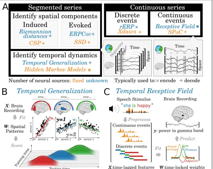
For example, mixed electrophysiological recordings (i.e. when neuronal responses randomly project onto the sensors, Fig. 4) are often modeled with spatial patterns time-locked to external events. For example, it is common to model the evoked response to an external event by fitting a series of linear models at each time-sample time-locked to the events. This approach hence results in a decoding score that varies over time _{(Cichy, Pantazis, & Oliva, 2014; King et} al., 2013)_{. A generalization of this method can be used to characterize the overall dynamics of} the neural responses _{(King & Dehaene, 2014; Meyers, Freedman, Kreiman, Miller, & Poggio,} 2008; Stokes et al., 2013) _{. The so-called Temporal Generalization method consists in testing} whether the models, independently fit at time each time-sample, are interchangeable with one another. Specifically, the ability of a model fit at time _{t to generalize to t’} determines whether the decoded mental representations is associated with a sustained or a changing pattern of brain activity. Similarly, Hidden Markov Models can be used to track sequence of brain responses by parametrically discretizing a fixed series of stages and fit their the onset and offset on the neural data _{(Borst & Anderson, 2015). Finally, it is also common to fit a linear model to neural} responses at each temporal and spatial sample separately, using a weighted combination of stimulus features_{(L. Gwilliams, Lewis, & Marantz, 2016; Hauk, Shtyrov, & Pulvermüller, 2008).} Overall, these supervised analyses help identifying and interpreting the dynamics and the overall sequence of evoked responses associated with a particular cognitive process.

The above methods focus on “evoked” spatial patterns - i.e. neural responses whose phases are consistent across repeated segments. By contrast, a number of decoding methods have been developed to identify “induced” spatial patterns - i.e. neural responses whose dynamics are not phase-locked to an external event. The decoding of induced activity is generally based on the spatial covariance of electrophysiological recordings. For example, the Common Spatial Pattern (CSP) method is a popular spatial filtering technique to identify the spatial pattern of neural activity that maximizes the discrimination between induced responses of two category of external events (e.g. left versus right hand) _{(Koles, Lazar, & Zhou, 1990).} Similarly, the Source Power Comodulation (SPoC) method extracts spatial patterns that are modulated by a continuous variable (e.g. hand position) _{(Dähne, Meinecke, et al., 2014).}

More recently, the decoding performance of induced decoders has proved to be improved by directly using the spatial covariance as a feature, without spatial filtering (Barachant, Bonnet, & Congedo, 2012; Farquhar, 2009) _{. This approach can be used without} specifying _{a priori the number of informative neural sources. However, such covariance matrices} must be properly linearized to take into account their symmetric and positive-definite structure when used with a linear model _{(Barachant, Bonnet, Congedo, & Jutten, 2013).}

2.2.2 Continuous time series.

Some cognitive processes may be particularly difficult to investigate within a segmented time-series framework. For example, auditory and speech processing involve rapid and overlapping stimulations. In such cases, it is thus common to model the neural dynamics with multiple “time-lags” of continuously-varying features (i.e. build an Hankel matrix _{(Almon, 1965;}

(13)

Ho & Kálmán, 1966) _{), in order to capture the possibility that some neural activity is time-locked} to specific events. For example, one can first preprocess an auditory waveform of recorded speech (i) to extract its continuously changing envelope as well as (ii) to annotate the onsets of individual words (Fig 7.C, _{(de Heer, Huth, Griffiths, Gallant, & Theunissen, 2017; Holdgraf et al.,} 2017)_{). A “receptive field” model can then be fit to the corresponding Hankel matrix in order to} isolate the neural responses to discrete events (e.g. word onsets) as well as to fluctuations in the continuously-changing speech envelope. This modeling is similar to the predominant approach in fMRI analysis, where the design matrix is convolved with a known impulse (i.e. the canonical hemodynamic response function). However, in the case of electrophysiology, the shape of the impulse response function is not known _{a priori and can indeed be vastly different} for different neurocognitive processes. The shape of electro-magnetic responses must thus be estimated from the data. Temporal receptive fields have been applied in a variety of contexts: they can be used to encode the average brain responses to categorical events (Regression-based Event Related Potentials, _{(de Heer et al., 2017; Smith & Kutas, 2015)) and} spectro-temporal patterns of visual and auditory inputs _{(Theunissen et al., 2001), and they can} also be used to decode overlapping sequences of neural correlates of discrete _(Rivet, Souloumiac, Attina, & Gibert, 2009; Theunissen et al., 2001) and continuously changing events (Dähne, Nikulin, et al., 2014)_.

2.3 Predicting sequences of computations.

In the last decade, the analytical tools reviewed above have been supplemented with models that aim to identify the sequence of computations necessary to efficiently produce cognitive operations. Indeed, with the recent rebirth of deep neural networks, a wide variety of computational architectures have been produced in the machine learning community. For example, state of the art computer vision models are now dominated by deep convolutional neural networks, which apply an extended series of non-linear transformations on the convolution of images, in order to detect objects from natural images.

The sequence of operations applied by such neural networks has been found to map with both the spatial _{(Cichy et al., 2016; Eickenberg et al., 2017; Gwilliams & King, 2017;} Kriegeskorte, 2015; Yamins et al., 2014) and the temporal organization _{(Cichy et al., 2016;} Gwilliams & King, 2017; van de Nieuwenhuijzen et al., 2013) of the visual system. Specifically, the early activity in the primary visual cortex is specifically and linearly correlated with the activation in superficial layers, whereas the later responses of the inferior temporal cortex are specifically and linearly related to the activation of the deep layers of these CNNs. This suggests that the computations applied by the human brain to solve a given task, as well as the order of those computations, may be modeled with deep neural networks trained to solve the same task.

Overall, these results confirm the long-predicted notion that the perceptual systems are organized as an extended computational hierarchy _{(Hubel & Wiesel, 1963; Riesenhuber &} Poggio, 1999)_{, and interestingly link machine learning and neuroscience within a common} computational framework.

(14)

Figure 7. Decoding and encoding neural sequences. A. The methods to track and decompose sequences of neural responses can be categorized between those based on independent segments of neural recordings (left) and those that additionally dissociate the overlapping effects of stimulation and behavior (right). A variety of spatial filtering techniques (i.e. linear combinations of sensors) have been proposed to extract oscillatory (induced) and average brain responses (evoked) locked to particular events. We implemented these methods together with dedicated tutorials in the MNE package _{(Gramfort et al., 2014). B.} Temporal generalization consists in fitting a spatial filter at each timesample locked to an event, and testing whether it can be used to decode the brain responses at all time-samples. This analysis can be used to determine whether a sustained decoding score results from a stable pattern of neural responses, or whether it reflects a series of transient neural responses. Adapted from _{(King & Dehaene, 2014) C. Temporal receptive fields consist in first} annotating the latent dimensions of that characterize the continuously-varying experimental variables - e.g. the spectral modulation of an acoustic waveform, the lexical categories of spoken words etc - (top left). These features are then transformed into a time-delay matrix whose linear modeling can be used to recover the temporal response profile of each feature (bottom right, Adapted from _{(Holdgraf et al., 2017)).}

(15)

Conclusion

Overall, the rapid development of machine learning provides a threefold promise to cognitive neuroscience. First, these tools support the automatization, denoising and summary of complex electrophysiological and neuroimaging time series. Second, these tools offer an operational ground to data-driven investigation: unanticipated patterns of data may be automatically identified from large datasets, without requiring the preface of human insight. Finally, machine learning and cognitive neuroscience share the common goal of identifying the elementary components of knowledge acquisition and information processing. The interface between cognitive neuroscience and machine learning thus leads to a mutual benefit. On the one hand, machine learning can help define, identify, and formalize the computations of the brain. On the other hand, cognitive neuroscience can help provide insights and principled directions to shape the computational architecture of complex cognitive processes _(Hassabis, Kumaran, Summerfield, & Botvinick, 2017; Lake, Ullman, Tenenbaum, & Gershman, 2017)_.

References

Almon, S. (1965). The Distributed Lag Between Capital Appropriations and Expenditures. Econometrica:

Journal of the Econometric Society, 33(1), 178–196.

Barachant, A., Bonnet, S., & Congedo, M. (2012). Multiclass brain–computer interface classification by

Riemannian geometry. IEEE Transactions on. Retrieved from

http://ieeexplore.ieee.org/abstract/document/6046114/

Barachant, A., Bonnet, S., Congedo, M., & Jutten, C. (2013). Classification of covariance matrices using a

Riemannian-based kernel for BCI applications. Neurocomputing, 112, 172–178.

Bastos, A. M., Usrey, W. M., Adams, R. A., Mangun, G. R., Fries, P., & Friston, K. J. (2012). Canonical

microcircuits for predictive coding. Neuron, 76(4), 695–711.

Benjamin, A. S., Fernandes, H. L., Tomlinson, T., Ramkumar, P., VerSteeg, C., Chowdhury, R., … Kording, K. P. (2017). Modern machine learning outperforms GLMs at predicting spikes.

https://doi.org/10.1101/111450

Borst, J. P., & Anderson, J. R. (2015). The discovery of processing stages: analyzing EEG data with

hidden semi-Markov models. NeuroImage, 108, 60–73.

Bose, A., & Recce, M. (2001). Phase precession and phase-locking of hippocampal pyramidal cells.

Hippocampus, 11(3), 204–215.

Boto, E., Holmes, N., Leggett, J., Roberts, G., Shah, V., Meyer, S. S., … Brookes, M. J. (2018). Moving

magnetoencephalography towards real-world applications with a wearable system. Nature,

555(7698), 657–661.

Branco, T., Clark, B. A., & Häusser, M. (2010). Dendritic discrimination of temporal input sequences in

cortical neurons. Science, 329(5999), 1671–1675.

Brincat, S. L., & Connor, C. E. (2004). Underlying principles of visual shape selectivity in posterior

inferotemporal cortex. Nature Neuroscience, 7(8), 880–886.

Buzsaki, G. (2006). Rhythms of the Brain. Oxford University Press.

Chichilnisky, E. J. (2001). A simple white noise analysis of neuronal light responses. Network, 12(2),

199–213.

Cichy, R. M., Khosla, A., Pantazis, D., Torralba, A., & Oliva, A. (2016). Comparison of deep neural

networks to spatio-temporal cortical dynamics of human visual object recognition reveals hierarchical

correspondence. Scientific Reports, 6, 27755.

(16)

Nature Neuroscience, ₁₇(3), 455–462.

Dähne, S., Meinecke, F. C., Haufe, S., Höhne, J., Tangermann, M., Müller, K.-R., & Nikulin, V. V. (2014). SPoC: a novel framework for relating the amplitude of neuronal oscillations to behaviorally relevant

parameters. _NeuroImage, ₈₆, 111–122.

Dähne, S., Nikulin, V. V., Ramírez, D., Schreier, P. J., Müller, K.-R., & Haufe, S. (2014). Finding brain

oscillations with power dependencies in neuroimaging data. _NeuroImage, ₉₆, 334–348.

Dehaene, S., & Cohen, L. (2007). Cultural recycling of cortical maps. _Neuron, ₅₆(2), 384–398.

de Heer, W. A., Huth, A. G., Griffiths, T. L., Gallant, J. L., & Theunissen, F. E. (2017). The Hierarchical

Cortical Organization of Human Speech Processing. _{The Journal of Neuroscience: The Official}

Journal of the Society for Neuroscience, ₃₇(27), 6539–6557.

Di Liberto, G. M., Di Liberto, G. M., O’Sullivan, J. A., & Lalor, E. C. (2015). Low-Frequency Cortical

Entrainment to Speech Reflects Phoneme-Level Processing. _{Current Biology: CB}, ₂₅(19),

2457–2465.

Donders, F. C. (1969). On the speed of mental processes. _{Acta Psychologica}, ₃₀, 412–431.

Eickenberg, M., Gramfort, A., Varoquaux, G., & Thirion, B. (2017). Seeing it all: Convolutional network

layers map the function of the human visual system. _NeuroImage, ₁₅₂, 184–194.

Ekman, M., Kok, P., & de Lange, F. P. (2017). Time-compressed preplay of anticipated events in human

primary visual cortex. _{Nature Communications}, ₈, 15276.

Farquhar, J. (2009). A linear feature space for simultaneous learning of spatio-spectral filters in BCI.

Neural Networks: The Official Journal of the International Neural Network Society, ₂₂(9), 1278–1285. Freiwald, W. A., & Tsao, D. Y. (2010). Functional compartmentalization and viewpoint generalization

within the macaque face-processing system. _Science, ₃₃₀(6005), 845–851.

Fries, P. (2005). A mechanism for cognitive dynamics: neuronal communication through neuronal

coherence. _{Trends in Cognitive Sciences}, ₉(10), 474–480.

Fyhn, M., Molden, S., Witter, M. P., Moser, E. I., & Moser, M.-B. (2004). Spatial representation in the

entorhinal cortex. _Science, ₃₀₅(5688), 1258–1264.

Girardeau, G., & Zugaro, M. (2011). Hippocampal ripples and memory consolidation. _{Current Opinion in}

Neurobiology, ₂₁(3), 452–459.

Gramfort, A., Luessi, M., Larson, E., Engemann, D. A., Strohmeier, D., Brodbeck, C., … Hämäläinen, M.

S. (2014). MNE software for processing MEG and EEG data. _NeuroImage, ₈₆, 446–460.

Gramfort, A., Papadopoulo, T., Baillet, S., & Clerc, M. (2011). Tracking cortical activity from M/EEG using

graph cuts with spatiotemporal constraints. _NeuroImage, ₅₄(3), 1930–1941.

Gwilliams, L., & King, J.-R. (2017). Performance-optimized neural network only partially account for the

spatio-temporal organization of visual processing in the human brain. _BioRxiv.

https://doi.org/_{10.1101/221630}

Gwilliams, L., Lewis, G. A., & Marantz, A. (2016). Functional characterisation of letter-specific responses

in time, space and current polarity using magnetoencephalography. _NeuroImage, ₁₃₂, 320–333.

Hafting, T., Fyhn, M., Molden, S., Moser, M.-B., & Moser, E. I. (2005). Microstructure of a spatial map in

the entorhinal cortex. _Nature, ₄₃₆(7052), 801–806.

Hämäläinen, M., Hari, R., Ilmoniemi, R. J., Knuutila, J., & Lounasmaa, O. V. (1993).

Magnetoencephalography—theory, instrumentation, and applications to noninvasive studies of the

working human brain. _{Reviews of Modern Physics}, ₆₅(2), 413–497.

Hassabis, D., Kumaran, D., Summerfield, C., & Botvinick, M. (2017). Neuroscience-Inspired Artificial

Intelligence. _Neuron, ₉₅(2), 245–258.

Hastie, T., Tibshirani, R., & Friedman, J. (2009). Unsupervised Learning. In T. Hastie, R. Tibshirani, & J.

Friedman (Eds.), _{The Elements of Statistical Learning: Data Mining, Inference, and Prediction} (pp.

485–585). New York, NY: Springer New York.

Haufe, S., Meinecke, F., Görgen, K., Dähne, S., Haynes, J.-D., Blankertz, B., & Bießmann, F. (2014). On

the interpretation of weight vectors of linear models in multivariate neuroimaging. _NeuroImage, ₈₇,

96–110.

Hauk, O., Shtyrov, Y., & Pulvermüller, F. (2008). The time course of action and action-word

comprehension in the human brain as revealed by neurophysiology. _{Journal of Physiology, Paris},

102(1-3), 50–58.

(17)

1084–1086.

Heeger, D. J., & Mackey, W. E. (2018, March 16). _{ORGaNICs: A Theory of Working Memory in Brains}

and Machines. _{arXiv [cs.AI]}. Retrieved from _{http://arxiv.org/abs/1803.06288}

Heeger, D. J., & Ress, D. (2002). What does fMRI tell us about neuronal activity? _{Nature Reviews.}

Neuroscience, ₃, 142.

Ho, B. L., & Kálmán, R. E. (1966). Effective construction of linear state-variable models from input/output

functions. _{At-Automatisierungstechnik}, ₁₄(1-12), 545–548.

Hochreiter, S., & Schmidhuber, J. (1997). Long short-term memory. _{Neural Computation}, ₉(8),

1735–1780.

Holdgraf, C. R., Rieger, J. W., Micheli, C., Martin, S., Knight, R. T., & Theunissen, F. E. (2017). Encoding

and Decoding Models in Cognitive Electrophysiology. _{Frontiers in Systems Neuroscience}, ₁₁, 61.

Hubel, D. H., & Wiesel, T. N. (1963). Shape and arrangement of columns in cat’s striate cortex. _The

Journal of Physiology, ₁₆₅, 559–568.

Hung, C. P., Kreiman, G., Poggio, T., & DiCarlo, J. J. (2005). Fast readout of object identity from

macaque inferior temporal cortex. _Science, ₃₁₀(5749), 863–866.

Huth, A. G., de Heer, W. A., Griffiths, T. L., Theunissen, F. E., & Gallant, J. L. (2016). Natural speech

reveals the semantic maps that tile human cerebral cortex. _Nature, ₅₃₂(7600), 453–458.

Jazayeri, M., & Afraz, A. (2017). Navigating the Neural Space in Search of the Neural Code. _Neuron,

93(5), 1003–1014.

Jones, M. W., & Wilson, M. A. (2005). Theta Rhythms Coordinate Hippocampal–Prefrontal Interactions in

a Spatial Memory Task. _{PLoS Biology}, ₃(12), e402.

Jun, J. J., Steinmetz, N. A., Siegle, J. H., Denman, D. J., Bauza, M., Barbarits, B., … Harris, T. D. (2017).

Fully integrated silicon probes for high-density recording of neural activity. _Nature, ₅₅₁(7679),

232–236.

Kamitani, Y., & Tong, F. (2005). Decoding the visual and subjective contents of the human brain. _Nature

Neuroscience, ₈(5), 679–685.

Kanwisher, N. (2001). Faculty of 1000 evaluation for Distributed and overlapping representations of faces

and objects in ventral temporal cortex. _{F1000 - Post-Publication Peer Review of the Biomedical}

Literature. https://doi.org/_{10.3410/f.1000496.16554}

Kao, J. C., Nuyujukian, P., Ryu, S. I., Churchland, M. M., Cunningham, J. P., & Shenoy, K. V. (2015).

Single-trial dynamics of motor cortex and their applications to brain-machine interfaces. _Nature

Communications, ₆, 7759.

King, J.-R., & Dehaene, S. (2014). Characterizing the dynamics of mental representations: the temporal

generalization method. _{Trends in Cognitive Sciences}, ₁₈(4), 203–210.

King, J. R., Faugeras, F., Gramfort, A., Schurger, A., El Karoui, I., Sitt, J. D., … Dehaene, S. (2013). Single-trial decoding of auditory novelty responses facilitates the detection of residual

consciousness. _NeuroImage, ₈₃, 726–738.

King, J.-R., Pescetelli, N., & Dehaene, S. (2016). Brain Mechanisms Underlying the Brief Maintenance of

Seen and Unseen Sensory Information. _Neuron, ₉₂(5), 1122–1134.

Kistler, W. M., & Gerstner, W. (2002). Stable propagation of activity pulses in populations of spiking

neurons. _{Neural Computation}, ₁₄(5), 987–997.

Koles, Z. J., Lazar, M. S., & Zhou, S. Z. (1990). Spatial patterns underlying population differences in the

background EEG. _{Brain Topography}, ₂(4), 275–284.

Kording, K. P., Benjamin, A., Farhoodi, R., & Glaser, J. I. (2018). The Roles of Machine Learning in

Biomedical Science. In _{Frontiers of Engineering: Reports on Leading-Edge Engineering from the}

2017 Symposium. National Academies Press.

Kriegeskorte, N. (2015). Deep Neural Networks: A New Framework for Modeling Biological Vision and

Brain Information Processing. _{Annual Review of Vision Science}, ₁, 417–446.

Kriegeskorte, N., & Kievit, R. A. (2013). Representational geometry: integrating cognition, computation,

and the brain. _{Trends in Cognitive Sciences}, ₁₇(8), 401–412.

Lake, B. M., Ullman, T. D., Tenenbaum, J. B., & Gershman, S. J. (2017). Building machines that learn

and think like people. _{The Behavioral and Brain Sciences}, ₄₀, e253.

Lebedev, M. A., & Nicolelis, M. A. L. (2006). Brain-machine interfaces: past, present and future. _{Trends in}

(18)

Liaw, A., Wiener, M., & Others. (2002). Classification and regression by randomForest. _{R News}, ₂(3), 18–22.

Lisman, J., & Idiart, M. (1995). Storage of 7 /- 2 short-term memories in oscillatory subcycles. _Science,

267(5203), 1512–1515.

Marr, D. (1982). Vision: A computational investigation into the human representation and processing of

visual information. _{WH San Francisco: Freeman and Company}. Retrieved from

https://mitpress.mit.edu/books/978-0-262-29037-1

Mesgarani, N., Cheung, C., Johnson, K., & Chang, E. F. (2014). Phonetic feature encoding in human

superior temporal gyrus. _Science, ₃₄₃(6174), 1006–1010.

Meyers, E. M., Freedman, D. J., Kreiman, G., Miller, E. K., & Poggio, T. (2008). Dynamic population

coding of category information in inferior temporal and prefrontal cortex. _{Journal of Neurophysiology},

100(3), 1407–1419.

Mineault, P. J., Khawaja, F. A., Butts, D. A., & Pack, C. C. (2012). Hierarchical processing of complex

motion along the primate dorsal visual pathway. _{Proceedings of the National Academy of Sciences}

of the United States of America, ₁₀₉(16), E972–E980.

Misaki, M., Kim, Y., Bandettini, P. A., & Kriegeskorte, N. (2010). Comparison of multivariate classifiers

and response normalizations for pattern-information fMRI. _NeuroImage, ₅₃(1), 103–118.

Moser, E. I., Kropff, E., & Moser, M.-B. (2008). Place cells, grid cells, and the brain’s spatial

representation system. _{Annual Review of Neuroscience}, ₃₁, 69–89.

Nishimoto, S., Vu, A. T., Naselaris, T., Benjamini, Y., Yu, B., & Gallant, J. L. (2011). Reconstructing Visual

Experiences from Brain Activity Evoked by Natural Movies. _{Current Biology: CB}, ₂₁(19), 1641–1646.

Olah, C., Satyanarayan, A., Johnson, I., Carter, S., Schubert, L., Ye, K., & Mordvintsev, A. (2018). The

Building Blocks of Interpretability. _Distill, ₃(3). https://doi.org/_{10.23915/distill.00010}

Price, C. J. (2010). The anatomy of language: a review of 100 fMRI studies published in 2009. _{Annals of}

the New York Academy of Sciences, ₁₁₉₁, 62–88.

Quiroga, R. Q., Nadasdy, Z., & Ben-Shaul, Y. (2004). Unsupervised spike detection and sorting with

wavelets and superparamagnetic clustering. _{Neural Computation}, ₁₆(8), 1661–1687.

Riesenhuber, M., & Poggio, T. (1999). Hierarchical models of object recognition in cortex. _Nature

Neuroscience, ₂(11), 1019–1025.

Ritchie, J. B., Brendan Ritchie, J., Kaplan, D., & Klein, C. (2017). Decoding The Brain: Neural Representation And The Limits Of Multivariate Pattern Analysis In Cognitive Neuroscience.

https://doi.org/_{10.1101/127233}

Rivet, B., Souloumiac, A., Attina, V., & Gibert, G. (2009). xDAWN algorithm to enhance evoked potentials:

application to brain-computer interface. _{IEEE Transactions on Bio-Medical Engineering}, ₅₆(8),

2035–2043.

Sahani, M., & Linden, J. F. (2003). How Linear are Auditory Cortical Responses? In S. Becker, S. Thrun,

& K. Obermayer (Eds.), _{Advances in Neural Information Processing Systems 15} (pp. 125–132). MIT

Press.

Shadlen, M. N., & Newsome, W. T. (1998). The variable discharge of cortical neurons: implications for

connectivity, computation, and information coding. _{The Journal of Neuroscience: The Official Journal}

of the Society for Neuroscience, ₁₈(10), 3870–3896.

Sigman, M., Cecchi, G. A., Gilbert, C. D., & Magnasco, M. O. (2001). On a common circle: natural scenes

and Gestalt rules. _{Proceedings of the National Academy of Sciences of the United States of}

America, ₉₈(4), 1935–1940.

Singer, W., & Gray, C. M. (1995). Visual feature integration and the temporal correlation hypothesis.

Annual Review of Neuroscience, ₁₈, 555–586.

Smith, N. J., & Kutas, M. (2015). Regression-based estimation of ERP waveforms: II. Nonlinear effects,

overlap correction, and practical considerations. _{Psychophysiology}, ₅₂(2), 169–181.

Sternberg, S. (1998). Discovering mental processing stages: The method of additive factors.

https://doi.org/_{1999-02657-014}

Stevenson, I. H., & Kording, K. P. (2011). How advances in neural recording affect data analysis. _Nature

Neuroscience, ₁₄, 139.

Stokes, M. G. (2015). “Activity-silent” working memory in prefrontal cortex: a dynamic coding framework.

(19)

Stokes, M. G., Kusunoki, M., Sigala, N., Nili, H., Gaffan, D., & Duncan, J. (2013). Dynamic coding for

cognitive control in prefrontal cortex. _Neuron, ₇₈(2), 364–375.

Theunissen, F. E., David, S. V., Singh, N. C., Hsu, A., Vinje, W. E., & Gallant, J. L. (2001). Estimating spatio-temporal receptive fields of auditory and visual neurons from their responses to natural

stimuli. _Network, ₁₂(3), 289–316.

Tybrandt, K., Khodagholy, D., Dielacher, B., Stauffer, F., Renz, A. F., Buzsáki, G., & Vörös, J. (2018).

High-Density Stretchable Electrode Grids for Chronic Neural Recording. _{Advanced Materials},

30(15), e1706520.

van de Nieuwenhuijzen, M. E., Backus, A. R., Bahramisharif, A., Doeller, C. F., Jensen, O., & van Gerven, M. A. J. (2013). MEG-based decoding of the spatiotemporal dynamics of visual category

perception. _NeuroImage, ₈₃, 1063–1073.

van Kerkoerle, T., Self, M. W., Dagnino, B., Gariel-Mathis, M.-A., Poort, J., van der Togt, C., & Roelfsema, P. R. (2014). Alpha and gamma oscillations characterize feedback and feedforward

processing in monkey visual cortex. _{Proceedings of the National Academy of Sciences of the United}

States of America, ₁₁₁(40), 14332–14341.

Van Steveninck, R., & Bialek, W. (1988). Real-time performance of a movement-sensitive neuron in the

blowfly visual system: coding and information transfer in short spike sequences. _{Proc. R. Soc}.

Retrieved from _{http://rspb.royalsocietypublishing.org/content/234/1277/379.short}

Varoquaux, G., Raamana, P. R., Engemann, D. A., Hoyos-Idrobo, A., Schwartz, Y., & Thirion, B. (2017).

Assessing and tuning brain decoders: Cross-validation, caveats, and guidelines. _NeuroImage,

145(Pt B), 166–179.

Wandell, B. A., Dumoulin, S. O., & Brewer, A. A. (2007). Visual field maps in human cortex. _Neuron,

56(2), 366–383.

Yamins, D. L. K., Hong, H., Cadieu, C. F., Solomon, E. A., Seibert, D., & DiCarlo, J. J. (2014). Performance-optimized hierarchical models predict neural responses in higher visual cortex.

Proceedings of the National Academy of Sciences of the United States of America, ₁₁₁(23), 8619–8624.

Zander, T. O., & Kothe, C. (2011). Towards passive brain-computer interfaces: applying brain-computer

interface technology to human-machine systems in general. _{Journal of Neural Engineering}, ₈(2),