HAL Id: tel-01145923
https://tel.archives-ouvertes.fr/tel-01145923
Submitted on 27 Apr 2015
HAL is a multi-disciplinary open access archive for the deposit and dissemination of sci-entific research documents, whether they are pub-lished or not. The documents may come from teaching and research institutions in France or abroad, or from public or private research centers.
L’archive ouverte pluridisciplinaire HAL, est destinée au dépôt et à la diffusion de documents scientifiques de niveau recherche, publiés ou non, émanant des établissements d’enseignement et de recherche français ou étrangers, des laboratoires publics ou privés.
Variarional data assimilation in the land surface model
ORCHIDEE using YAO
Hector Simon Benavides Pinjosovsky
To cite this version:
Hector Simon Benavides Pinjosovsky. Variarional data assimilation in the land surface model OR-CHIDEE using YAO. Earth Sciences. Université Pierre et Marie Curie - Paris VI, 2014. English. �NNT : 2014PA066590�. �tel-01145923�
1
Université Pierre et Marie Curie
Ecole doctorale de Sciences de l’environnement de l’Ile de France
Spécialité
Méthodes statistiques et modèles inverses
Sujet de la thèse
Assimilation variationnelle des données dans le modèle de surface
continentale ORCHIDEE grâce au logiciel YAO
Présentée par
Hector Simon Benavides Pinjosovsky
Dirigée par
Sylvie Thiria et Catherine Ottlé
Présentée et soutenue publiquement le 27 mars 2014 Devant le jury composé de
Mme. Sylvie Thiria LOCEAN/IPSL Directeur de thèse
Mme. Catherine Ottlé LSCE/CEA/IPSL Co-directeur de thèse
Mme. Isabelle Herlin INRIA Rapporteur
Mme. Dominique Courault INRA Rapporteur
M. Fouad Badran CEDRIC/CNAM Examinateur
M. Hervé Le Treut LMD/CNRS Examinateur
3
Résumé
Un modèle de surface continentale (LSM en anglais) est un modèle numérique décrivant les échanges d'eau et d'énergie entre la surface terrestre et l'atmosphère. La physique de la surface de la terre comprend une vaste collection de processus complexes. L'équilibre entre la complexité du modèle et sa résolution, confronté à des limitations de calcul, représente une question fondamentale dans le développement d'un LSM. Les observations des phénomènes étudiés sont nécessaires afin d’adapter la valeur des paramètres du modèle à des variables reproduisant le monde réel. Le processus d'étalonnage consiste en une recherche des paramètres du modèle qui minimisent l’écart entre les résultats du modèle et un ensemble d'observations. Dans ce travail, nous montrons comment l'assimilation variationnelle de données est appliquée aux bilans d'énergie et d'eau du modèle de surface continentale ORCHIDEE afin d’étalonner les paramètres internes du modèle. Cette partie du modèle est appelé SECHIBA. Le logiciel YAO est utilisé pour faciliter la mise en œuvre de l'assimilation variationnelle 4DVAR.
Une analyse de sensibilité a été réalisée afin d'identifier les paramètres les plus influents sur la température. Avec la hiérarchie des paramètres obtenue, des expériences jumelles à partir d'observations synthétiques ont été mises en œuvre. Les résultats obtenus suggèrent que l'assimilation de la température de surface a le potentiel d'améliorer les estimations de variables, en ajustant correctement les paramètres de contrôle. Enfin, plusieurs assimilations ont été faites en utilisant des observations de données réelles du site SMOSREX à Toulouse, France. Les expériences faites en utilisant différentes valeurs initiales pour les paramètres, montrent les limites de l'assimilation de la température pour contraindre les paramètres de contrôle. Même si l'estimation des variables est améliorée, ceci est dû à des valeurs finales des paramètres aux limites des intervalles prescrit de la fonction de coût. Afin de parvenir à un minimum, il faudrait permettre aux paramètres de visiter des valeurs irréalistes. Les résultats montrent que SECHIBA ne simule pas correctement simultanément la température et les flux et la relation entre les deux n’est pas toujours cohérente selon le régime (ou les valeurs des paramètres que l’on utilise). Il faut donc travailler sur la physique pour mieux simuler la température. En outre, la sensibilité des paramètres à la température n’est pas toujours suffisante, donnant une fonction de coût plate dans l’espace des paramètres prescrit. Nos résultats montrent que le système d'assimilation mis en place est robuste, puisque les résultats des expériences jumelles sont satisfaisants.
Le couplage entre l'hydrologie et la thermodynamique dans SECHIBA doit donc être revu afin d'améliorer l'estimation des variables. Une étude exhaustive de l'erreur des mesures doit être menée afin de récupérer des termes de pondération dans la fonction de coût. Enfin, l'assimilation d'autres variables telles que l'humidité du sol peut maintenant être réalisée afin d'évaluer l'impact sur les performances de l’assimilation.
5
Abstract
A land surface model (LSM) is a numerical model describing the exchange of water and energy between the land surface and the atmosphere. Land surface physics includes an extensive collection of complex processes. The balance between model complexity and resolution, subject to computational limitations, represents a fundamental query in the development of a LSM. With the purpose of adapting the value of the model parameters to values that reproduces results in the real world, measurements are necessary in order to compare to our estimations to the real world. The calibration process consists in an optimization of model parameters for a better agreement between model results and a set of observations, reducing the gap between the model and the available measurements. Here we show how variational data assimilation is applied to the energy and water budgets modules of the ORCHIDEE land surface model in order to constrain the model internal parameters. This part of the model is denoted SECHIBA. The adjoint semi-generator software denoted YAO is used as a framework to implement the 4DVAR assimilation.
A sensitivity analysis was performed in order to identify the most influent parameters to temperature. With the parameter hierarchy resolved, twin experiments using synthetic observations were implemented for controlling the most sensitive parameters. Results obtained suggest that land surface temperature assimilation has the potential of improving the output estimations by adjusting properly the control parameters. Finally, several assimilations were made using observational meteorology dataset from the SMOSREX site in Toulouse, France. The experiments implemented, using different prior values for the parameters, show the limits of the temperature assimilation to constrain control parameters. Even though variable estimation is slightly improved, this is due to final parameter values are at the edge of a variation interval in the cost function. Effectively reaching a minimum would require allowing the parameters to visit unrealistic values. SECHIBA does not correctly simulates simultaneously temperature and fluxes and the relationship between the two is not always consistent according to the regime (or parameter values that are used). We must therefore work on the physical aspects to better simulate the temperature. Likewise, the parameter sensitivity to temperature is not always sufficient, giving as a result a flat cost function.
Our results show that the assimilation system implemented is robust, since performances results in twin experiments are satisfactory. The coupling between the hydrology and the thermodynamics in SECHIBA must be reviewed in order to improve variable estimation. An exhaustive study of the prior errors in the measurements must be conducted in order to retrieve more adapted weighing terms in the cost function. Finally, the assimilation of other variables such as soil moisture should be performed to evaluate the impacts in constraining control parameters
7
Remerciements
A deep gratitude to all those who in one way or another were involved in the development process of my work and in the writing of this manuscript. To all the people that during these recent years helped me to overcome the difficulties of this project.
9
Index
CHAPTER 1 INTRODUCTION
LAND SURFACE MODELS. OBJECTIVES AND ORGANIZATION OF THE THESIS ... 13
1.1 INTRODUCTION ... 13
1.2 COMPONENTS OF LAND SURFACE MODELS ... 14
1.2.1WATER PROCESSES ... 14
1.2.2SOIL THERMODYNAMICS ... 17
1.3 IMPORTANCE OF REPRESENTING THE PHYSICS OF THE SOIL SURFACE CORRECTLY ... 23
1.4 CHALLENGES IN LSM REPRESENTATION ... 23
1.4.1.SURFACE HETEROGENEITY ... 23
1.4.2NUMERICAL REPRESENTATION ... 24
1.4.3.MATHEMATICAL REPRESENTATION AND MODEL CALIBRATION ... 24
1.5 THESIS CHALLENGES ... 26
1.5.1.STATE OF THE ART IN THE USE OF LST TO CONSTRAIN LSM ... 26
1.5.2GENERAL OBJECTIVES ... 27
1.5.3ORGANIZATION ... 28
CHAPTER 2 DESCRIPTION OF THE LAND SURFACE MODEL ORCHIDEE AND DATASETS ... 31
2.1. ORCHIDEE ... 31 2.1.1MODULES ... 31 2.1.2BIOSPHERE CHARACTERIZATION ... 32 2.2 SECHIBA... 34 2.2.1FORCING... 34 2.2.2ENERGY BUDGET ... 35 2.2.3HYDROLOGICAL BUDGET ... 37 2.2.4.SECHIBAPARAMETERS ... 38 2.3 DATA ... 40
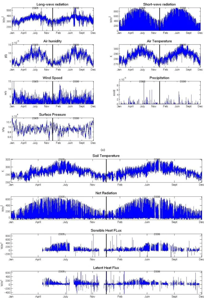
2.3.1.EDDY COVARIANCE MEASUREMENTS ... 40
2.3.2SMOSREX ... 44
CHAPTER 3 THEORETICAL PRINCIPLES OF VARIATIONAL DATA ASSIMILATION ... 47
3.1 INTRODUCTION AND NOTATION ... 47
3.2 ADJOINT METHOD ... 50
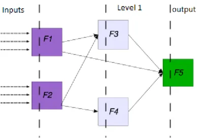
3.3. REPRESENTING A MODEL AND ITS ADJOINT THROUGH A MODULAR GRAPH ... 51
3.3.1.DEPLOYMENT OF A MODULAR GRAPH ... 54
3.4. DIAGNOSTIC TOOLS FOR THE ASSIMILATION SYSTEM ... 55
3.4.1TEST THE CORRECTNESS OF THE ADJOINT MODEL ... 55
3.4.2.TEST THE CORRECTNESS OF THE COST FUNCTION GRADIENTS ... 56
3.4.3.DERIVATIVE TEST ... 56
3.5. SUMMARY ... 57 CHAPTER 4
10
THE YAO APPROACH: THEORETICAL ASPECTS AND IMPLEMENTATION OF SECHIBA-YAO 1D ... 59
4.1 INTRODUCTION ... 59
4.2 YAO APPROACH ... 60
4.3. CREATING A PROJECT WITH YAO ... 61
4.3.1INPUT /OUTPUT MANAGEMENT ... 62
4.3.2DIAGNOSTIC TOOLS FOR THE GENERATED PROJECT ... 63
4.4. DEVELOPMENT OF SECHIBA-YAO 1D ... 63
4.4.1IMPLEMENTATION OUTLINE ... 65
4.4.2DIRECT MODEL VALIDATION ... 68
4.4.3ADJOINT MODEL VALIDATION ... 72
CHAPTER 5 SENSITIVITY ANALYSIS OF THE SECHIBA-YAO 1D MODEL USING FLUXNET DATASET ... 77
5.1 INTRODUCTION ... 77
5.2 VARIATIONAL SENSITIVITY ANALYSIS ... 79
5.2.1.SENSITIVITY ANALYSIS WITH LAND SURFACE TEMPERATURE ... 79
CHAPTER 6 TWIN EXPERIMENTS WITH SECHIBA-YAO 1D USING FLUXNET MEASUREMENTS ... 101
6.1 INTRODUCTION ... 101
6.2 EXPERIMENT DEFINITION ... 101
6.3. RESULTS ... 103
6.3.1EFFECT OF THE OBSERVATION SAMPLING ... 103
6.3.2EFFECT OF RANDOM NOISE IN THE OBSERVATION ... 105
6.3.3EFFECT OF THE CONTROL PARAMETER SET SIZE ... 106
6.4. DISCUSSION ... 109
CHAPTER 7 REAL MEASUREMENTS STUDY USING SMOSREX DATASET ... 111
7.1 INTRODUCTION ... 111
7.2 KEY PARAMETERS TO PERFORM THE OPTIMIZATION ... 112
7.3 LST DATA ASSIMILATION WITH PARAMETER STANDARD VALUES ... 113
7.3.1.SIMULATED VS.OBSERVED MEASUREMENTS ... 113
7.3.2.BRIGHTNESS TEMPERATURE SENSITIVITY ANALYSIS ... 119
7.3.3.BRIGHTNESS TEMPERATURE ASSIMILATION DURING A SINGLE DAY ... 120
7.3.4.BRIGHTNESS TEMPERATURE ASSIMILATION DURING A WEEK ... 122
7.3.5.DISCUSSION ... 126
7.4 LST VARIATIONAL DATA ASSIMILATION WITH DIFFERENT PRIOR VALUES ... 126
7.4.1.SIMULATED VS.OBSERVED MEASUREMENTS ... 126
7.4.2.BRIGHTNESS TEMPERATURE SENSITIVITY ANALYSIS ... 129
7.4.3.BRIGHTNESS TEMPERATURE ASSIMILATION DURING A SINGLE DAY ... 130
7.4.4.BRIGHTNESS TEMPERATURE ASSIMILATION DURING A WEEK ... 132
7.5. ANALYSIS OF THE ASSIMILATION SYSTEM THROUGH TWIN EXPERIMENTS ... 133 7.6 CONCLUSION
11
CHAPTER 8
CONCLUSION AND PERSPECTIVES ... 139
REFERENCES ... 145 FIGURE INDEX ... 151 TABLE INDEX ... 155 APPENDIX A ... 157 APPENDIX B ... 161 APPENDIX C ... 171
13
Chapter 1 Introduction
Land Surface Models. Objectives and
Organization of the Thesis
1.1 Introduction
A land surface model (LSM) is a numerical model describing the exchange of water and energy between the land surface and the atmosphere. It is used in weather and climate modeling to simulate different processes at the Earth’s surface, such as the water, carbon fluxes and the thermodynamics from the surface to the atmosphere. The atmospheric model provides the forcing above the surface (incoming radiation, precipitation, atmospheric temperature and humidity). In exchange, LSM calculates surface variables (soil temperature, soil moisture, leaf area index, etc…) and outgoing fluxes to the atmosphere.
A good description of surface processes is essential for weather and climate applications. Located at the boundary between the atmosphere and the soil, LSM provides the link between several scientific disciplines subject to intense research in the hydrological, atmospheric, and remote sensing communities. LSM contains a set of general components, as mentioned in Liu and Gupta, 2007. First, we have the system boundary, which sets the limit conditions to model variables, allowing the separation of internal components of a system from external entities. Second, forcing inputs describe the model variables modified by the external components of the model: these are the inputs of the model. Next, the initial states of the model define a more realistic scenario for the state variables. We also have the model parameters, which are part of the equations describing the physical phenomena. Finally, the model structure contains a description of how the model is decomposed in its elementary processes and the discretization path used.
14
Principal components of LSM and their associated physics are explained in the next section.
1.2 Components of land surface models 1.2.1 Water processes
The soil surface regulates the exchanges between water and plants. The ability of soil to hold water is related to its constitution. It is composed of particles that can be large or compact. Depending on soil composition, its ability to absorb water is different. Very dry soil cracks and becomes very compact. It cannot store water, which escapes through the large cracks on the surface, and runs off. Therefore in such areas the vegetation is limited or nonexistent. The water balance defines the soil water content by integrating all the water that comes in and all the water that leaves the soil (Musy et al., 1991).
All movements of water in the soil depend on its structure and its state: the infiltration process consists in vertical water movement that enters the soil through tiny cracks together. This phenomenon occurs in the first meters below the surface of the Earth. This movement maintains the reserves of deep water. The infiltration process modifies in a drastic and instantaneous way the pressure and the water content in the ground surface.
This process is conditioned by several factors of which the most significant comes from the soil, through its hydrodynamics characteristics, its texture and its structure. In addition, specific conditions can determine the infiltration process: the water flow rate, precipitation intensity, etc.
Hydrological Cycle
The hydrological cycle is a concept that encompasses the phenomena of movement and renewal of water on Earth. Concepts in this section are taken from Musy et al., 2003. This definition implies that the mechanisms governing the hydrological cycle does not only occur one after the other, but there are also concurrent. Under the effect of solar radiation, water evaporates from the soil, oceans and other surfaces such as lakes, rivers, etc. The rise of moist air through the atmosphere facilitates its cooling, which is necessary to bring it to saturation, causing condensation of water vapor into droplets forming clouds in the presence of condensation nuclei. Then the water vapor, transported and stored temporarily in the clouds, is returned to oceans and continents through rainfall. Part of the rainfall can be intercepted by plants and then be partially restored by evaporation. Intercepted rain not evaporated can
15
further reach the ground (NOAA National Weather Service Jetstream).
Depending on soil conditions, water might evaporate from the ground, run off, infiltrate into the ground where it can be stored as soil moisture or leak into deeper areas to contribute to the renewal of groundwater reserves. Flow from the latter can reach the surface at springs or streams. Evaporation from the soil, rivers, and plant transpiration complete the cycle.
Figure 1. 1 Water moves through the Earth, changing state and drifting to the atmosphere, the oceans and over the land surface and underground, in different processes that coexist. It is subject to complex processes; among them we cite precipitation, evaporation, transpiration,
interception, runoff, infiltration, percolation, storage and subsurface flows. These various mechanisms are made possible by the incoming surface energy. (Source: NOAA National
Weather Service Jetstream).
Water Balance
We can represent the continuous process of the water cycle in three general phases: precipitation, surface runoff, infiltration and evaporation. In each phase we found a transport of water and sometimes a change of state. The water balance equation takes these phases into account, and it is expressed as follows
E R P
S [mm] (1.1)
With P the precipitation (liquid and solid), S the resources (accumulation) in the previous period (infiltration, soil moisture, snow, ice), R the surface runoff and groundwater
16
flow and E the evapotranspiration, defined as the integration of evaporation and transpiration. Precipitation is the rain water falling on the surface of the earth, both in liquid and solid form. In order to produce condensation in the atmosphere, water vapor must reach the dew point by cooling or by increasing its pressure. In addition, the presence of certain microscopic nuclei allows water droplets to condense. The source of these nuclei may be oceanic (chlorides, in particular NaCl produced by sea evaporation), continental (dust, smoke and other particles carried out by ascending air currents) or cosmic (meteoric dust). The onset of precipitation is favored by the coalescence of water drops. The increase in mass gives them a gravitational force sufficient to overcome the updrafts and turbulence of the air and to reach the ground. Finally, the course of raindrops or snowflakes must be short enough to prevent evaporation of the total mass.
Evaporation is defined as the transition from liquid to vapor. Water bodies, such as lakes and oceans and vegetation cover are the main sources of water vapor. The main factors governing the evaporation are the solar radiation, the wind and the soil moisture. The term evapotranspiration includes evaporation and plant transpiration. It is a fundamental component of the hydrological cycle and its study is essential to determine the water resources of a region or watershed. In general, specific analysis of evaporation will be made to balance studies and management of water by plants. Evaporation of the soils is produced at the surface. Transpiration is produced by plants essentially by the leaves with water extracted from the soil in the root zone. Both processes occur simultaneously. The evapotranspiration process is conditioned by the evaporative power, which expresses the extraction capacity of water, performed by the atmosphere on the ground-vegetation system. This evaporative power is determined by the evaporative demand of the air and the system's ability to satisfy this request, depending on the availability of water and plant physiology.
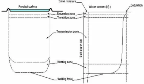
Infiltration refers to the downward movement of water from the land surface into the soil. Infiltration can occur naturally following precipitation, or can be induced artificially through structural modifications in the ground surface (Musy et al., 1991). The infiltration process is characterized by the water influx in the soil. This influx is called infiltration regime, which is defined also as the flux density q. The infiltration rate can be influenced by the soil properties like its porosity, the hydraulic conductivity and the initial humidity rate.
The precipitation penetrating the soil creates several zones, as shown in Fig.1.2. These zones are: the saturation zone at the soil surface; the transmission zone, which is characterized by constant water content; the wetting zone, in which the water content is decreased and ends
17
up in the last zone and finally the wetting front, characterized by an abrupt decrease in the water content.
Figure 1. 2 Soil profile and the different types of saturation zones. (Musy and Soutter, 1991). The soil water capacity is expressed as a depth of water that can be infiltrated per unit of time. If rainfall supplies water at a rate that is greater than the infiltration capacity, water will infiltrate at the capacity rate, with the excess either being ponded, moved as surface runoff, or evaporated. If rainfall supplies water at a rate less than the infiltration capacity, all of the incoming water volume will infiltrate. In both cases, as water infiltrates into the soil, the capacity to infiltrate more water decreases and approaches a minimum capacity. When the supply rate is equal to or greater than the capacity to infiltrate, the minimum capacity will be approached more quickly than when the supply rate is much less than the infiltration capacity.
1.2.2 Soil thermodynamics
Formalism and notations presented in Musy and Soutter (1991) are adopted in this part of the work. Soil thermodynamics describes the different processes representing soil temperature in space and time. Temperature is a variable characterizing the degree of thermal distribution and the level of body heat. Many physical, chemical and biological processes are strongly influenced by temperature. The occurrence of thermal gradients results in transfers by heat diffusion, liquid flows, soil aeration, drainage and exchanges with the atmosphere. They are all conditioned by the thermal state of the soil. The soil temperature at a specific point depends on two types of phenomena: on one hand the energy exchange with the outside environment, determining the amount of total energy stored in the ground, and on the other, a
18
complex series of transfer processes of heat, depending on the specific thermal properties of soil, which determines energy distribution in the ground.
Energy transfer
Heat transfers are energy exchanges, following three types of energy physical processes: radiation, thermal and latent. They are defined based on the formulation of their dynamics and a conservation law. The main parameters involved in the description of the thermal behavior of a soil are those used to characterize the stored energy. These values depend on the specific thermal properties of the various components of the soil.
The thermal properties of the soil are conditioned by the characteristics of their texture and structure. One of these parameters is Ct, the heat capacity of a body, which is defined by
dT dQ
, where dQ is the energy-heat required to raise the body temperature per dT. The isobaric heat capacity is denoted by
CT
Cp
(1.2) were Cp is the storage capacity of body heat per unit mass and temperature. Internal exchanges of energy, thermal energy or sensible heat transfer in soil occur in two different processes: thermal conduction and convection.
Figure 1. 3 Thermal conduction between two solid (left) and thermal convection between a solid and a fluid (right). (Source: Musy and Soutter, 1991)
19
conduction and convection, denoted as JD
and JV
, respectively (Fig.1.3). Both are based on different physical exchange heat processes. Their dynamics is described by different laws, depending on the number of phases involved. The total heat flux is defined as
V D T J J
J
(1.3) Thermal conduction is a diffusion process in which the transfer of energy is due to the difference in temperature between two regions of a medium or between two media in contact without displacing material. The thermal agitation is transmitted from one molecule or atom giving a portion of its kinetic energy to its neighbor. This transfer process ends only when a heat balance is reached. The heat flux transferred by conduction is proportional to a gradient of decreasing temperature, defined by the Fourier law:
T grad K
JD T (1.4) The Fourier coefficient or thermal conductivity Kt in Eq.1.4 represents the resistance of
the material to the propagation of heat by thermal conduction, expressing its ability to transfer heat from one point to another. Thermal conductivity depends on the composition of the material, its mineral content and organic matter as well as the shape of its constituent particles. It varies in space and in time as a function of variations in air moisture.
In thermal convection, the transfer of energy takes place in the molecules located at the boundary between a solid and a fluid in motion. The transfer is carried out by the molecular agitation and fluid mass displacement. This heat transfer is expressed in terms of Ti, the
thermal density, is described as ) ( S W pw w i c T T T
(1.5) Where w is the water density and cpw is the isobaric heat capacity density. Theexchanged heat by the movement of the fluid must be associated with the law expressing the fluid dynamics. The sensible heat flux transferred by thermal convection Jv
is written using the following expression
q T
Jv i (1.6)
In natural convection, heat is transferred by density currents that run through the fluid under the effect of disparities in temperature at the solid-fluid interface. In this case, the
20
sensible heat flux is expressed as
T grad D c
Jv W pw T (1.7) where DT is the molecular diffusivity. The temperature gradient determines the transfer of
thermal energy from one phase to the other. The dynamic law expressing the total sensible heat flux results from the sum of conduction and convection transferred by heat flow.
The general equation of exchange of sensible heat is the combination of the dynamic law and the principle of continuity. It can be expressed in terms of thermodynamics principles.
z K gradT D div grad D div t X (1.8)
div K gradT div D grad t T cpw T w (1.9) The first equation (Eq.1.8), includes the transfer of water under the influence of the potential gradient of water and the thermal gradient. Here, D is the water transfer diffusivity, DX is the thermal gradient diffusivity and is the quantity of water in the soil. The second equation (Eq.1.9) is the general equation of heat flux to which we add a latent heat flux due to evaporation flow. Here, D and are terms related to the latent heat flux diffusivity of soil.
Energy budget
The sun is the main source of energy reaching the surface of the Earth. In a single year, the Earth system (atmosphere, surfaces, and oceans) absorbs sunlight driving photosynthesis, evaporation, and melts snow and ice, among other processes. The heat collected is not uniform across surface of the Earth. The atmosphere and ocean balance the energy received by the Sun through surface evaporation, rainfall, ocean circulation, winds, etc. Mean temperature in Earth doesn’t increase relentlessly because the surface and the atmosphere are simultaneously radiating heat back to space. This net flow of energy is known as the energy budget.
Variations in the average temperature reflect the balance of energy exchanges between the soil and the outside environment. These exchanges occur at the soil-atmosphere interface in the form of radiant energy, heat and latent.
The net radiation is the difference between the amount of incoming radiation and the amount of outgoing radiation by the surface. Reflectivity of the atmosphere and the ground
21
surface determines the amount of radiation the surface will absorb. This reflectivity is known as albedo, a coefficient that determines the reflected solar radiation for a particular surface. Albedo varies with surfaces, leading to net heating inequities throughout the Earth: more incoming sunlight is received in the summer hemisphere compared to the winter hemisphere. When the Earth is subject to a flow of radiant energy, it absorbs a portion, reflects another and transmits the remainder, as it is described in Figure 1.4.
Figure 1. 4 Global Earth Energy Budget. (Source: NASA)
The energy radiation budget exchange to the surface is expressed by the net radiation, which is represented by
h h b b
n R R R R
R (1.10)
Where Rh↓ is the incident solar radiation, Rh ↑ is the reflected solar radiation, Rb is the
radiation emitted by the surface. Rn can be expressed also as the global radiation Rg product
with the surface albedo α, following the equation
SW T LW Rn 4 1 (1.11)Another element of the energy budget is represented by the exchange of sensible heat. The exchange of thermal agitation energy by convection is the main process of sensible heat
22
transfer between the ground and the atmosphere. The convection exchange takes place simultaneously by natural convection (heat distribution) and by forced convection, as a result of the mechanical stirring action of the wind. The sensible heat flux H is represented by
gradT D
C
H a pa T (1.12)
where ρa is the air density, Cpa is the isobaric specific heat capacity and Dt is the thermal
diffusivity. Another type of exchange occurs in the form of latent heat, wherein the energy has been converted by a phase change of heat transfer and thus being associated with a mass transfer. Sensible heat converts during this process to latent heat, transferred by the vapor mass flow. This flow can be expressed in general as the product of the concentration gradient, the volume fraction coefficient Vvap and an exchange coefficient De. Diffusive and convective
effects transfer of water vapor in the air are then defined as
vap e
vap D grad V
q
(1.13) The latent heat flux associated to the water vapor mass flow is expressed as
vap e pa a p grad D C LE (1.14) where LE is the vaporization latent heat, pvap is the evaporation pressure and γ is the
psychrometric constant, defined as γ ≈ 0.66.10-2 N/m2K
Formulation
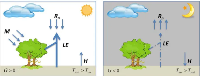
The energy budget provides the balance between the balance of radiation and heat exchange. It is calculated from the following equation:
W/m 2
G LE H M Rn (1.15)Rn is the net radiation, M represents the part of the radiation energy absorbed by the
system and used for photosynthesis, and it is usually neglected. G represents the radiation energy converted into heat and stored in the system, after deducting the sensible heat flux H and latent heat flux LE.
23
Figure 1. 5 Daylight and night energy budgets. (Source: Musy et Soutter (1991)).
1.3 Importance of representing the physics of the soil surface correctly
Land surface model helps us to understand the processes that trigger the precise climate in a region, by analyzing its internal interactions. We are able to understand the current climate locally but also the factors that generate a specific climate in other regions. Fluxes between soil and the atmosphere can have non-local effects. In addition, climatic conditions into the future can be predicted. Its accuracy depends on the degree of precision with which the model represents the physics reality and the assumptions about the future factors that climate will encounter.
Furthermore, LSM provides data not directly available or difficult to interpolate. Models compute different estimates answering questions about what processes will affect a particular region in the future.
1.4 Challenges in LSM representation
The land surface physics includes an extensive collection of complex processes. The balance between model complexity and resolution, subject to computational limitations, represents a fundamental question in the development of LSM. By increasing the comprehension of physical phenomena, LSM can grow into a more complex model adding new processes extrapolated from the environment. In the next section, some of the complexities found in most LSM are presented.
1.4.1. Surface heterogeneity
24
particles that determine its inherent characteristics. Its ability to retain water and its density varies drastically depending on the percentage of primitive components (sand, silt, or clay) or structure (ash, fine, or coarse sand). There may be several types of soil in a small area, with their associated features, especially water content. Omission of surface spatial heterogeneity in a LSM can cause errors in flux estimation (Courault et al., 2010, Olioso et al., 2005). Spatial variations in surface heterogeneity are imperative in order to guarantee an accurate simulation of the land-surface fluxes. The sub-grid scale land surface heterogeneity must be parameterized in the surface scheme so that the land characteristics are accounted for in the model (Manrique et al, 2013).
1.4.2 Numerical representation
The development process of a physical model into numerical software extends from the physical world to the mathematical model, then to the computational algorithm and finally to the computer implementation, involves a number of approximations: physical effects may be discarded, continuous functions replaced by discretized ones and real numbers replaced by finite precision representations. In consequence, approximation is in the core of scientific software and cannot be neglected. It is important to manage them judiciously.
The accuracy of a computation determines how close the computation (affected by random errors) comes to the true mathematical value. It indicates, therefore, the correctness of the result. In particular, numerical verification, as Rump (1983) mentioned, is required to give confidence that the computed results are acceptable. The precision of a computation reflects the exactness of the computed result without reference to the meaning of the computation. It is, therefore, the number of significant digits affected by round-off error. Arithmetic expressions and variable assignment always produce approximation errors, due to the nature of the floating point arithmetic. Approximation modes in computer software will determines the precision in the several operations made in the model coded. This precision is independent of the code, data or machine. When building LSM numerical representation, we have to be aware of these errors and track their propagation.
1.4.3. Mathematical representation and model calibration
Representing a physical model need the definition of its numerical and its discretized form. In terms of simplicity, models have to include the least amount of parameters needed to achieve a good performance in its estimates (parsimonious models). Model building is best
25
achieved by starting with the simplest structure and gradually and accurately increasing the complexity as needed to improve model performance (Wainwright et al., 2004). However, there is no metric that quantifies the estimate improvement by increasing complexity.
The parameters that are required to compute real world outputs estimations are best defined by a model structure that best represent the processes measured in the real world. In practice, this can be difficult to achieve. With our model, we may be interested in trying to reconstruct past events that need some parameters that are impossible to measure. In that case we may have to make reasonable assumptions based on indirect evidence. These assumptions can be made in order to define the model from reality. Several of them will and can be wrong, nonetheless they are necessary for the model development. The output of the model depends completely on the validity and scope of these assumptions. A parameter measurement must be chosen based on the impact the variation of a parameter has on the model output, or the model sensitivity to this parameter.
According to Kirkby et al (1992) there are two types of parameters in a model: the physical parameters which define the physical structure of the model, and the process parameters or multiplying factors, which weigh the magnitude of variables in the model. The physical parameters are determined from experimental measurements. The process parameters are defined from a calibration and adjustment process. In both cases, the definition of the initial parameter value can be a difficult task. The physical parameters are determined on small scales, and then they are extrapolated, given the spatial and temporal variability in the region we are working.
With the purpose of adapting the value of the parameter to a value that reproduces the real world, measurements of a phenomenon are necessary in order to compare to our model estimates. The calibration process consists in an optimization process against a measure of the agreement between model results and a set of observations. It allows the agreement between the model and the available measures; however, this process may give clues to poorly defined processes in the model (Pipunic et al., 2008).
With respect to the LSM, many works have focused on the calibration of the models based on soil moisture measurements, since it is an observation easy to obtain, it is directly measured with high frequency and is the solution of the water budget. There are many sources of data available in a wide range of ecosystem.
26
1.5 Thesis Challenges
1.5.1. State of the art in the use of LST to constrain LSM
Several works regarding the calibration of LSM based on LST measurements demonstrate the improvement in fluxes estimation, when constraining model parameters.
In Castelli et al. (1999), a variational data assimilation approach is used to include surface energy balance in the estimation procedure as a physical constraint (the adjoint technique). The authors work with satellite data, where soil skin temperature is directly assimilated. As a conclusion, constraining the model with such observation improves model fluxes estimations, with respect to in situ measurements.
In Huang et al. (2003) the authors developed a one-dimensional land data assimilation scheme based on ensemble Kalman filter, used to improve the estimation of soil temperature profile. They conclude that the assimilation of LST into land surface models is a practical and effective way to improve the estimation of land surface state variables and fluxes.
Reichle et al. (2010) performed an assimilation of satellite-derived skin temperature observations using an ensemble-based, offline land data assimilation system. Results suggest that retrieved fluxes provide modest but statistically significant improvements. However, they noted strong biases between LST estimates from in situ observations, land modeling, and satellite retrievals that vary with season and time of day. They highlighted the importance to take these biases properly, or else large errors in surface flux estimates can result. In Ghent et al. (2011), the authors investigate the impacts of data assimilation on terrestrial feedbacks of the climate system. Assimilation of LST helped to constrain simulations of soil moisture and surface heat fluxes. Another study by Ghent et al. 2011, investigates the effect that data assimilation has on terrestrial feedbacks to the climate system. The authors state that representation of highly complex biophysical processes in LSMs over highly heterogeneous land surfaces with limited collections of mathematical equations, and the tendency of over parameterization, infers a degree of uncertainty in their predictions. Assimilation of land surface temperature (LST) to constrain simulations of soil moisture and surface heat fluxes can be integrated into the model to update a quantity simulated by the model with the purpose of reducing the error in the model formulation. The correction applied is derived from the respective weights of the uncertainties of both the model predictions and the observations. The results found in this research suggest that there is potential for LST to act as surrogate for assimilating other state variables into a land surface scheme.
27
Ridler et al. (2012) tested the effectiveness of using satellite estimates of radiometric surface temperatures and surface soil moisture to calibrate a Soil–Vegetation–Atmosphere Transfer (SVAT) model, based on error minimization of temperature and soil moisture model outputs. Flux simulations were improved when the model is calibrated against in situ surface temperature and surface soil moisture versus satellite estimates of the same fluxes.
In Bateni et al. (2013), the full heat diffusion equation is employed as constrain, in the variational data assimilation scheme. Deviations terms of the evaporation fraction and a scale coefficient are added as penalization terms in the cost function. Weak constraint is applied to data assimilation with model uncertainty, accounting in this way for model error. The cost function in this experience contains a term that penalizes deviation from prior values. When assimilating LST into the model, the authors proved that the heat diffusion coefficients are strongly sensitive to specific deep soil temperature. As a conclusion, it can be seen that the assimilation of LST can get a remarkable improvement in the model simulated flows.
1.5.2 General objectives
In this work, the LSM used is ORCHIDEE (Krinner et al., 2005), most specifically the part of the model computing the energy and hydrology balance (SECHIBA, Ducoudré et al, 1993). These models are introduced in Chapter 2.
The general objective of this thesis is to constrain the SECHIBA model parameters by assimilating measurements products in a 4DVAR assimilation system. The parameters, once constrained, allow the model to improve state variables estimation when comparing them to measurements.
From this general purpose, several specific objectives arise, as mandatory steps to implement an effective assimilation system, flexible enough to assimilate different observations and constraining at the same time different model parameters. These specific objectives are:
1. Study of SECHIBA and implementation into YAO: the understanding of the model physics through its standard Fortran code implementation is a mandatory step, in order to extract model dynamics and principal components. By knowing this, the implementation of SECHIBA in YAO can be made, by defining a modular graph representing the model dynamics and physics of the model. Our implementation of SECHIBA in YAO is called SECHIBA-YAO 1D. Once our model is coded, the direct model is verified comparing its
28
output with the original model. The adjoint model is verified by performing a sensitivity analysis, allowing us to obtain, in addition, a parameter hierarchy of the most influential parameter in the estimation of land surface temperature. SECHIBA-YAO 1D aims to run 4DVAR assimilation.
2. Validate the assimilation system, by implementing twin experiments. The idea is to test the robustness of the assimilation system, by computing variable and parameter performances. This phase highlights also the limits of the model when varying the control parameter set
3. Improve model estimation by performing a 4D-VAR assimilation of land surface temperature, using in situ measurements of SMOSREX site, in Toulouse, France. Available measurements of brightness temperature are compared with an equivalent form of temperature estimation added to SECHIBA, constraining model parameters to improve the simulation of the model variables, such as latent heat flux, sensible heat flux, net radiation, brightness temperature and soil moisture.
1.5.3 Organization
The thesis is organized such that the theoretical support is presented first, in Chapters 1 to 4. Experiment results concerning sensitivity analysis and variational data assimilation are presented in Chapters 5 to 7. Conclusions of the thesis are presented in Chapter 8. Finally, complementary information is presented in the Appendix section.
In Chapter 1, the introduction to land surface models and the nub of the thesis is presented. In Chapter 2, the land surface model used in this work (ORCHIDEE) is introduced, and more specifically SECHIBA and its main components and features. Equations governing the energy and hydrologic budget computed with SECHIBA are listed. In addition, data sources used in this work are introduced: FLUXNET network stations and SMOSREX in situ measurements.
Chapter 3 concerns variational data assimilation theoretical aspects. Additionally, the modular graph approach to represent models is presented. It is explained how an equivalent of the adjoint and tangent linear model is obtained, by computing the forward and the backward of the model through a modular graph decomposition. This approach is the basic idea of the YAO software, serving as a framework to implement SECHIBA variational data assimilation. In Chapter 4, the YAO approach is presented. This software served us as an adjoint semi
29
generator. Principal components of a YAO project are introduced, as well as the input/output data management. Finally, a general guide of how SECHIBA model was implemented in YAO is introduced. The different steps from the model conceptualization to the testing phase are explained in detail, serving as a guide to future implementations.
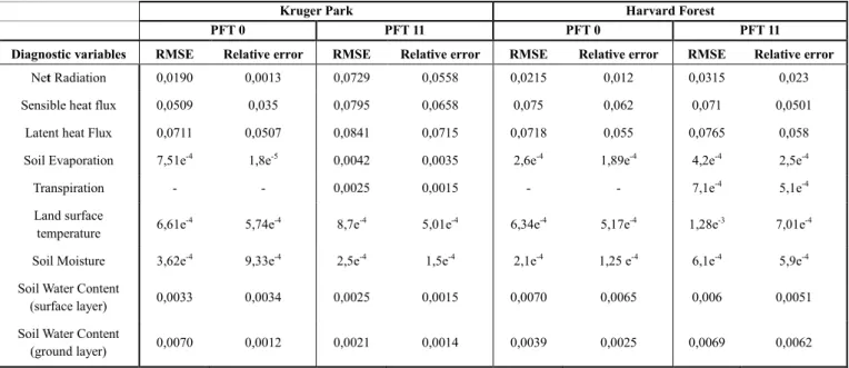
In Chapter 5, once the adjoint of SECHIBA is obtained using its YAO representation, we perform a variational sensitivity analysis with the idea of validating the adjoint of the model, by comparing the gradients obtained with SECHIBA-YAO 1D to the ones computed with finite differences, using the direct model outputs. In addition, we build a parameter hierarchy in order to determine the most influential parameters in the computation of land surface temperature. The sensitivity study was performed using FLUXNET sites (Kruger Park and Harvard Forest).
In Chapter 6, twin experiments are presented, using the FLUXNET data set. Different scenarios were tested in different experiments in order to account for the effect of assimilating synthetic observations of land surface temperature. In this chapter we show the potential of our assimilation system by using land surface temperature as observation.
In Chapter 7, assimilation of in situ measurements is presented using the SMOSREX site forcing. With different scenarios, this chapter shows the performance of assimilating land surface temperature with different initial conditions of parameters, time frames, among others. The idea is to show if the optimization of land surface temperature allows to constrain our model parameters and to better simulate surface fluxes.
Finally, in Chapter 8, the conclusion and perspectives of this work are presented. In addition, challenges related to the implementation of SECHIBA into YAO are mentioned.
31
Chapter 2
Description of the Land Surface Model
ORCHIDEE and datasets
2.1. ORCHIDEE
ORCHIDEE is a model representing the continental biosphere and its different processes, comprising the simulation of soil and vegetation mechanism and simulating different fluxes between the soil-atmosphere interface (Polcher et al., 1998, Krinner et al., 2005, Brender, 2012). ORCHIDEE has different time scales: energy and matter has a 30-minutes time scale. Species competition processes at 1-year time scale. The vegetation is grouped into 13 Plant Functional Type (PFT). The equations governing the processes are general, with specific parameters for each PFT. ORCHIDEE is used in a grid-point mode (one given location), forced with the corresponding local half hourly gap-filled meteorological measurements.
2.1.1 Modules
SECHIBA (Schématisation des Echanges Hydriques à l'Interface Biosphère-Atmosphère) (Ducoudré et al, 1993) is a biophysical model. It calculates the radiation and energy budgets of the surface, and the soil water budget every half hour. The energy and water fluxes between the atmosphere and the ground integrate all the vegetation layers; the retrieved temperature represents the canopy ensemble and the soil surface. The main fluxes modeled are the sensible and latent heat flux between the atmosphere and biosphere, the soil temperature and the water reservoirs evolution, the stomata conductance and gross primary productivity of the canopy.
32
STOMATE (Saclay Toulouse Orsay Model for the Analysis of Terrestrial Ecosystems) is a biogeochemical model. It represents the process related to the carbon cycle, such as carbon dynamics, the allocation of photosynthesis (Friedlingstein et al, 1999), respiration and growth maintenance, heterotrophic respiration (Ruimy et al., 1993) and phenology (Botta, 1999). STOMATE simulates the dynamics of continental carbon with no time every day. It links between processes at short time scales determined by SECHIBA and slower processes described by the following module.
LPJ (Lund-Potsdam-Jena) (Sitch et al, 2003) is a model of global dynamics of the vegetation. It incorporates the phenomena of interspecific competition for sunlight, fire occurrence, seedling establishment, plant mortality, and deduce the dynamic long-term (annual time step) of vegetation.
2.1.2 Biosphere Characterization
The surface model SECHIBA aims at representing the water and energy exchanges at the land surface. However, for a given moisture condition, they are highly dependent on soil type and vegetation cover. ORCHIDEE considers the diversity of a given ecosystem by defining 13 Plant functional Type (PFT). The vegetation is classified according to their ecophysiologic characteristics. Twelve common PFT exists, plus the bare soil; they are presented in Table 2.1. This classification depends on several parameters such as the appearance of the plant (tree or herb), the type of leaf (needle or leaves), the method of photosynthesis (C3 or C4) and the phenology type.
The different functional groups of plants and bare soil can coexist on the same mesh. A PFT is not intended to represent a plant species in particular but rather to regroup it, after several functional similarities. This will set the main functional characteristics such as height,
LAI, etc; and thus represent plant diversity around the world.
LAI (Leaf Area Index) is the total ratio of leaf area of a canopy over an area of soil. It is
expressed in m2 of leaf area per m2 of soil. For each mesh point, a fraction of PFT f
k is defined
as the vegetation fraction percent covering the studied location, verifying that 13 1
1 k k f . Each
fraction is modulated by a maximum max
k
f and by a corresponding LAI with the following equation: 13 , 2 ) 1 , . 2 min( . max f LAI k fk k k (2.1)
33
13 2 max max 1 1 ( ) k k k f f f f (2.2) If we have a LAI less than 0.5, we reduce linearly the vegetation fraction to zero for aLAI equal to zero and we increase equally the fraction of bare soil. Evolution of a LAI for each
PFT is bounded by minimum and maximum values which are assigned in Table 2.1. These values are reached according to the change in soil and vegetation temperatures
PFT Description Foliage Climate
0 Bare Soil - -
1 Rain forest sempervirens Persistent Tropical
2 Rainforest deciduous - Tropical
3 Temperate forest of conifers sempervirens Persistent Temperate 4 Temperate forest sempervirens Persistent Temperate
5 Temperate forest deciduous - Temperate
6 Boreal coniferous forest sempervirens Persistent Boreal
7 Boreal deciduous - Boreal
8 Boreal coniferous forest deciduous - Boreal
9 Herbaceous C3 C3 -
10 Herbaceous C4 C4 -
11 Agricultural C3 C3 -
12 Agricultural C4 C4 -
Table 2. 1 ORCHIDEE's Plant functional type description (d’Orgeval 2006)
In Table 2.2, h represents the prescribed vegetation height in meters, humcste is the root
profile coefficient (in m-1), rk is the structural resistance (in s.m-1), Tmin and Tmax are maximum
and minimum values of soil temperature at 50 cm and LAImax and LAImin are the maximum
and minimum values of LAI for each vegetation fraction.
Energy balance is solved once, with a subdivision only for latent heat flux in bare soil evaporation, interception and transpiration for each type of vegetation. Water balance is computed for each vegetation type given that, for a particular location, infiltration and evaporation will be different.
34
PFT h humcste rk LAImin LAImax Tmin Tmax
0 0 0 0 0 0 275.15 273.15 1 30 0.8 25 8 8 296.15 300.15 2 30 0.8 25 0 8 296.15 300.15 3 20 1 25 4 4 278.15 288.15 4 20 0.8 25 6 6 278.15 288.15 5 20 0.8 25 0 6 278.15 288.15 6 15 1 25 4 4 278.15 288.15 7 15 1 25 0 6 278.15 288.15 8 15 0.8 25 0 4 278.15 288.15 9 0.5 4 2.5 1 5 280.15 288.15 10 0.6 4 2 0 4 284.15 294.15 11 1 4 2 0 6 280.15 288.15 12 1 4 2 0 4.5 284.15 294.15
Table 2. 2 ORCHIDEE's plant functional type principal parameters (d’Orgeval 2006)
2.2 SECHIBA
Our study focuses on the vertical hydrological processes and the energy budget modeled in SECHIBA module. The other two modules of ORCHIDEE (i.e. STOMATE and LPJ) were not active. We chose to make simple assumptions concerning the modeling of vegetation cover. In order to do that, SECHIBA can be used decoupled from STOMATE.
2.2.1 Forcing
SECHIBA uses a time step of 30 minutes to represent the physical processes. The spatial resolution is determined by the atmospheric forcing used. For simulating surface fluxes and water movement in soil, SECHIBA must receive a number of input data from the atmosphere. They come either from observation data in a point or a region or from a general circulation model. Atmospheric information can only come from meteorological data which are often a combination of observations and modeling results. The data set is called an atmospheric forcing and the simulation mode is called forcing offline, which is imposed on the model simulation. However no feedback from the surface to the atmosphere is possible.
The relief of the surface is not reproduced in this model but is taken into account implicitly in the variability of atmospheric forcing or in the general circulation model (GCM). Thus, only the vegetation has an impact on the turbulence near the surface.
35
Variable Description Unit
Ta 2-meters air temperature K
qa 2-meters air humidity kg.kg −1
WN Wind speed at 10 meters (u) m.s−1
WE Wind speed at 10 meters (v) m.s−1
Psurf Surface pressure Pa
SWdown Short wave Incident Radiation (sun radiation) W.m−2
LWdown Long wave Incident Radiation (infrared radiation) W.m−2
Pliq Rain kg.m−2 .s−1
Psnow Snow kg.m−2 .s−1
Table 2. 3 Input Variables received by SECHIBA
Variables forcing SECHIBA are summarized in Table 2.3. In forcing mode, the air temperature and humidity are generally given at 2 meters and the wind at 10 meters. Corrections, especially for the wind speed, must be applied to compute a correct friction coefficient and turbulent fluxes.
2.2.2 Energy Budget
The dynamic of the fluxes modeled in the energy budget are presented in Fig 2.1. Fluxes equations and descriptions are summarized in Table 2.4.
Figure 2. 1 Energy Balance
The energy budget main fluxes are part of the energy equation, which has the following form
G H LE
Rn (2.3)
36
energy consumed by the evaporation from the surface or received by condensation on the surface, H corresponds to sensible heat flux or energy (received or dissipated to the surface) exchanged by convection between the surface and the air and G is the exchanged heat flux between soil surface and depth. In Fig.2.1 T corresponds to transpiration, E is the evaporation and Rlw+Rsw correspond to the incoming and outgoing long wave and shortwave incident solar
radiations. All these fluxes are expressed in W.m-2.
Flux Equation Description
Radiation LW net SW net net R R R (2.4)
SW
SW SW net R R kalbedo 1 (2.5)
LW
surf LW LW net R R R kemis (2.6)Rsw is the shortwave incident radiation
SW
is the surface albedo
kemis is the surface emissivity multiplying factor to be
optimized
RLW is the thermal radiation
LW surf
R is the thermal radiation emitted by surface
kalbedo is a multiplying factor weighing the effect the SW
has in the computation of SW surf
R . This parameter is
optimized
Soil heat flux 2
2 z T C t T cond capa k k (2.7)
λ is the soil conductivity, C the soil heat capacity and T the soil temperature.
The soil is discretized on 7 thermal layers. The layers have constant depths so that the first layer has a characteristic time of 30 minutes and the last of 2 hours.
kcapa and kcond are multiplying factors weighing the
parameters λ and C. They are both part of the control parameter set Turbulent Fluxes Aerodynamic Resistance ) . ( log10 z0 Cd z0 k overheight d a Z C U r 0 1 (2.8)
Cd is the drag coefficient. =0.41 is the Von Karman
Constant
z0 the roughness length and kz0 is a multiplying factor to
be optimized.
U is the normalized wind (m.s-1),
Sensible heat flux P( s a) a T T c r H (2.9)
H is proportional to the temperature gradient in the
surface-atmosphere interface.
ρ the air density (kg.m-3),
Cp the air heat capacity (J.kg-1.K-1) and Ta and Ts the air
and surface temperature in Kelvin
Latent Heat Flux air sol d q q C U LE (2.10)
LE integrates evaporation and transpiration.
corresponds to a coefficient integrating evaporation and transpiration resistance coefficients.
In SECHIBA, LE is divided in three components: Bare soil evaporation, interception loss and transpiration
Bare Soil Evaporation
r1=hs.rsolcste pot s a E U r r E . ' 1 1 1 (2.11)
E’pot is the potential evaporation, Us the soil humidity
computed in the hydrological balance, r1 is the bare soil
evaporation resistance,
rsolcste equal to 33000 s.m-2, representing the resistance for
bare soil square meter. This parameter is taken in the control parameter set. hs is dry soil height.
37 Interception loss pot a k k k k k E r r I I I E . ' 1 1 . , min max (2.12)
Ik is the foliage intercepted water and Ik
max is the maximum quantity that can be intercepted (Ik LAI.0.1mm
max ), rk the vegetation structural resistance, given by Table 2.2
Vegetation Stomata Resistance 0 0 1 k c a R R R LAI r n SW n SW k k rveg k (2.13)
krveg is a multiplying factor, weighing the calculation of the
vegetation resistance to transpiration. This parameter is optimized.
R0=12-5 W.m-2 , a=2.3.10-2kg.m-3 and λ=1.5. n
SW
R is the net solar radiation: SW SW n
SW R
R (1 ) . δc is the
atmosphere water vapor deficit: cmax( qs(Ta)qa,0).
Transpiration
solsat air
d k
k f U C q q
T 3 (2.14) Transpiration is computed for each vegetation fraction.
3
is a coefficient equivalent to the vegetation stomata
resistance
Table 2. 4 Energy budget fluxes
2.2.3 Hydrological Budget
The SECHIBA version used in this work models the hydrological budget based on a two-layer soil profile (Choisnel model, 1977). The soil layers correspond to the surface and the bottom of the soil. The total depth of the layers corresponds to the plants root depth. The soil has a unique type, with a total depth of dpucste = 2m. The bottom layer of soil acts like a
bucket that fills with water from the top layer. When the top layer is empty with no water (due to evaporation, drainage to the lower layer, or lack of precipitation), this layer disappears. When rainfall exceeds the evaporation losses, they recreate a wet surface, allowing it to evaporate. If the water quantity is about to saturate the two soil layers, the top layer disappears again and excess water is removed by runoff.
The soil fluxes, as they are modeled in SECHIBA, are presented in Fig 2.2. The different operations to obtain the fluxes are summarized in Table 2.3.
Figure 2. 2 Specific variables involved in hydrological budget computing (d’Orgeval, 2006). In Fig.2.2, Wu is the water content in the top layer, Wl is the water content in the bottom