Full polarization study of SiO masers at 86 GHz

(1)

HAL Id: hal-00016435

https://hal.archives-ouvertes.fr/hal-00016435

Submitted on 5 Jan 2006

HAL is a multi-disciplinary open access

archive for the deposit and dissemination of

sci-entific research documents, whether they are

pub-lished or not. The documents may come from

teaching and research institutions in France or

abroad, or from public or private research centers.

L’archive ouverte pluridisciplinaire HAL, est

destinée au dépôt et à la diffusion de documents

scientifiques de niveau recherche, publiés ou non,

émanant des établissements d’enseignement et de

recherche français ou étrangers, des laboratoires

publics ou privés.

Full polarization study of SiO masers at 86 GHz

Fabrice Herpin, Alain Baudry, Clemens Thum, Dave Morris, Helmut

Wiesemeyer

To cite this version:

Fabrice Herpin, Alain Baudry, Clemens Thum, Dave Morris, Helmut Wiesemeyer. Full polarization

study of SiO masers at 86 GHz. Astronomy and Astrophysics - A&A, EDP Sciences, 2006, 450-2,

pp.667-680. �10.1051/0004-6361:20054255�. �hal-00016435�

(2)

ccsd-00016435, version 1 - 5 Jan 2006

(DOI: will be inserted by hand later)

Full polarization study of SiO masers at 86 GHz

F. Herpin

1

, A. Baudry

1

, C. Thum

2

, D. Morris

2,3

and H. Wiesemeyer

2

1 _{Observatoire Aquitain des Sciences de l’Univers, Laboratoire d’Astrodynamique, d’Astrophysique et d’A´eronomie de} Bordeaux, CNRS/INSU UMR n◦_{5804, BP 89, 33270, France}

2 _{IRAM, 300 rue de la Piscine, Domaine Universitaire, 38406 Saint Martin d’H`eres, France} 3 _{Present address: Raman Research Institute, 560080 Bangalore, India}

the date of receipt and acceptance should be inserted later

Abstract.We study the polarization of the SiO maser emission in a representative sample of evolved stars in order to derive an estimate of the strength of the magnetic field, and thus determine the influence of this magnetic field on evolved stars. We made simultaneous spectroscopic measurements of the 4 Stokes parameters, from which we derived the circular and linear polarization levels. The observations were made with the IF polarimeter installed at the IRAM 30m telescope. A discussion of the existing SiO maser models is developed in the light of our observations. Under the Zeeman splitting hypothesis, we derive an estimate of the strength of the magnetic field. The averaged magnetic field varies between 0 and 20 Gauss, with a mean value of 3.5 Gauss, and follows a 1/r law throughout the circumstellar envelope. As a consequence, the magnetic field may play the role of a shaping, or perhaps collimating agent of the circumstellar envelopes in evolved objects.

Keywords. Maser: SiO – polarization– survey – stars:

late-type, evolution, magnetic field

1. Introduction

The prodigious mass loss observed in numerous and widespread evolved stars make these objects the main recycling agents of the interstellar medium, and thus one of the most im-portant objects in the Universe. Even though our knowledge of evolved stars has considerably improved over recent years, some of their main characteristics remain insufficiently under-stood (see the review by Herwig 2003): which mechanisms are responsible for their drastic change of geometry when evolving to the Planetary Nebula (hereafter PN) stage ? What is power-ing so efficiently the mass loss and could the magnetic field play a major role ?

Important information about the physics and chemistry prevailing in the circumstellar envelope (hereafter CSE) of evolved stars can be retrieved from radiowave line emission of molecules, specially from maser emission (see the review by Bujarrabal 2003). These envelopes can be probed at differ-ent depths through the study of three masing molecules, OH, H2O and SiO. Our current knowledge indicates that:

– OH radiation traces the outer part of the envelope, at

1000-10000 AU from the central star;

– H2O molecules are located at intermediate distances, i.e. a few 100 AU;

– SiO maser emission comes from the inner regions of the

envelope, between 5 to 10 AU (a few stellar radii R⋆).

The SiO maser emission is produced in small gas cells, and is known to be polarized. The polarization (circular or linear) and angle of the emission can be measured and thus improve our knowledge of these objects. In addition, studying the maser polarization can shed light on the maser theory itself. As ex-plained further in this paper, several uncertainties in the theory make data interpretation often difficult, and new observational data are helpful. One of the most interesting quantities that can be derived from polarization measurements is the stellar mag-netic field. According to theory (e.g. Elitzur 1996 or 2002), measurement of the maser radiation polarization can lead to an estimation of the magnetic field strength B and can reveal its spatial structure (via interferometric observations). In sin-gle dish observations, all of the maser components get smeared within the beam and only the mean value of B along the line of sight (B//) can be derived. Only SiO masers are capable of

tracing the magnetic field as close as ∼ 5 AU from the central star. But if SiO masers are to be used as a B-field tracer, we first need to give evidence that SiO masers are reliable B-field tracers. This requires more detailed theories than available to-day. Nevertheless, we tentatively derive in this work the field strength in the CSE inner layers of several evolved stars.

Research on astronomical masers polarization is very ac-tive but is made difficult both by the lack of specific instru-mental facilities and by the excitation and propagation of the masers themselves. Until now, numerous polarimetric observa-tions of OH masers have been done, several of H2O masers, but few of SiO maser emission. Few SiO polarimetric observa-tions have been done with VLBI giving the very first images of the magnetic field in some objects (e.g. Kemball & Diamond 1997 in TX Cam). Most of the early SiO studies were done

(3)

in linear polarization. The first complete SiO polarimetric ob-servations were performed by Johnson & Clark (1975), then by Troland et al. (1979); emission was found to be typically 15-30 % linearly polarized and to exhibit no circular polariza-tion. Barvainis, McIntosh & Predmore (1987), and McIntosh et al. (1989) measured circular polarization of 1 − 9 % in sev-eral stars. Circular (0-4 %) and linear (3.7-9.7 %) polarizations were measured in VY CMa by McIntosh, Predmore & Patel (1994). Later, Kemball & Diamond (1997) made the first image of the magnetic field in the atmosphere of TX Cam, measuring a circular polarization level of 5 % with some features showing polarization up to 30-40 %.

It must be stressed that SiO, as H2O, is a non-paramagnetic species. Zeeman splitting exists but the sublevels overlap; the effect is thus undetectable and hence only net polarization can be used to trace the magnetic field. The current status of our knowledge on the magnetic field strength can be summarized as follows:

– between 1000-10000 AU, B// ∼ 5 − 20 mG (OH masers,

e.g. Kemball & Diamond 1997, Szymczak & Cohen 1997);

– at a few 100 AU from the star, B// ∼ a few 100 mG

(H2O masers, e.g. Vlemmings, Diamond & van Langevelde 2001, Vlemmings, van Langevelde & Diamond 2005);

– at 5-10 AU, B// ∼ 5 − 10 G (SiO masers; Kemball &

Diamond 1997, in TX Cam).

The main purpose of this work is to measure and analyze the SiO maser polarization in terms of magnetic field strength in a representative sample of evolved stars. Our observations are presented in Section 2; they include simultaneous spectro-scopic measurements of the 4 Stokes parameters. The results for individual stars are discussed in Section 3. In Section 4, we compare our data with predictions from existing SiO maser models and initiate a discussion on the validity of these mod-els. Within the limitations of one of these models we derive the magnetic field strength and try to determine the role of the magnetic field. More broadly, a summary of the magnetic field topic in evolved stars is also given in Section 4. In Section 5 we give some concluding remarks.

2. Observations

An electromagnetic plane wave is defined by two components (horizontal and vertical):

eH(z, t) = EHej(ωt−kz−δ) (1)

eV(z, t) = EVej(ωt−kz) (2)

where δ is the phase difference between horizontal and ver-tical components.

Its energy flux is described by the 4 Stokes parameters:

I =< EH2> + <EV2> (3)

Q =< EH2> − < EV2> (4)

U = 2 < EHEVcos δ > (5)

V = 2 < EHEVsin δ > (6)

From these parameters, one deduces:

– the circular polarization rate pC= V/I

– the linear polarization rate pL=

p

Q2_{+ U}2_/_I

– the polarization angle χ = arctan(U/Q)₂

The linear/circular polarization rate is sometimes called the linear/circular fractional polarization.

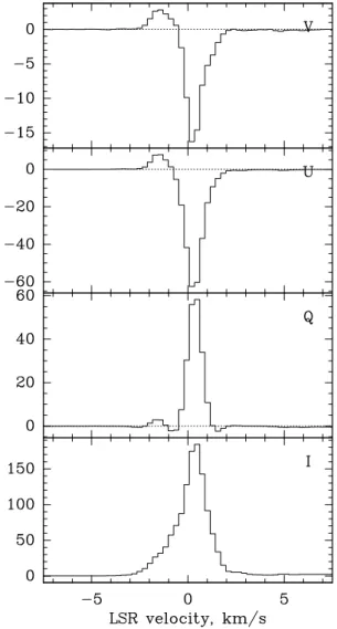
Fig. 1. V, U, Q and I Stokes parameters for R Leo. I, V, U and

Q are given in Kelvins (T a⋆_{; the conversion factor is 6 Jy/K).}

We present here spectroscopic measurements of the 4 Stokes parameters (see Fig. 1). The observations were made with the IF polarimeter installed at the IRAM 30m telescope on Pico Veleta, Spain (Thum et al. 2003). Simultaneous mea-surements of I, U, Q, V allow us to calculate I, pL, pCand χ for

each velocity channel. The polarization angle calibration (i.e. the sign of Stokes U) was verified by observations of the Crab Nebula. Moreover, planets (polarization of planets is negligi-ble at our frequency) have been used to check the instrumental polarization on the optical axis.

The instrumental beam polarization is known to be stronger in Stokes Q and U than in Stokes V (known to be ≤ 2-3%, see Thum et al. 2003, comparable to our sensitivity as stated elsewhere). If some detections from sources with weak pLare

(4)

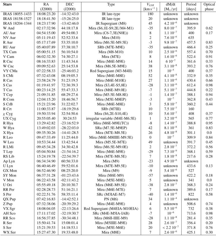
Table 1. Stars observed in this work. The stellar type is derived from the literature as are the mass loss rates (e.g. Loup et al.

1993) and the period (e.g. AAVSO data).

Stars RA DEC Type VLS R dM/dt Period Optical

(J2000) (J2000) [km s−1_] _[M

⊙/yr] [days] phase

IRAS 18055-1433 18:08:23.20 -14:32:43.0 IR late-type 180 unknown unknown IRAS 18158-1527 18:18:41.50 -15:26:25.0 IR late-type 20 unknown unknown IRAS 18204-1344 18:23:17.90 -13:42:46.0 IR Supergiant (M8) 45 4.2 10−6 _unknown

W And 02:17:32.96 44:18:17.8 Mira (S6,1E-S9,2E/M4-M1) -35 8.0 10−7 _395.9 _0.62

AU Aur 04:54:15.00 49:54:00.3 Mira (C6-7,3E(N0E)) 8 1.1 10−7 ₄₀₀ _0.17

NV Aur 05:11:19.43 52:52:33.6 Mira (M10) 2 7.6 10−6 ₆₃₅

R Aur 05:17:17.69 53:35:10.0 Mira (M6.5E-M9.5E) -3 9.8 10−7 _457.5 _0.83

RU Aur 05:40:07.89 37:38:10.7 SRb (M7E-M9E) -35 unknown 466.4 0.25 TX Cam 05:00:51.15 56:10:54.0 Mira (M8-M10) 10 2.5 10−6 _557.4 _0.70

V Cam 06:02:32.30 74:30:27.1 Mira (M7E) 8 1.6 10−6 _522.4 _0.91

R Cnc 08:16:33.83 11:43:34.6 Mira (M6E-M9E) 14 6 10−7 _361.6 _0.33

W Cnc 09:09:52.63 25:14:53.8 Mira (M6.5E-M9E) 38 3.1 10−8 _393.2 _0.76

VY CMa 07:22:58.33 -25:46:03.2 Red Supergiant (M3-M4II) 15 10−5 ₄₀₀ _0.37

S CMi 07:32:43.08 08:19:05.3 Mira (M6E-M8E) 52 4.1 10−8 _332.9 _0.35

R Cas 23:58:24.79 51:23:19.5 Mira (M6E-M10E) 27 1.1 10−6 _430.4 _0.66

S Cas 01:19:41.97 72:36:39.3 Mira (S3,4E-S5,8E) -28 3.1 10−6 _612.4 _0.98

T Cas 00:23:14.25 55:47:33.3 Mira (M6E-M9.0E) -7 5.1 10−7 _444.8 _0.22

T Cep 21:09:31.85 68:29:27.6 Mira (M5.5E-M8.8E) -1 1.4 10−7 _388.1 _0.94

R Com 12:04:15.20 18:46:56.7 Mira (M5E-M8EP) -3 10−7 _362.8 _0.43

S CrB 15:21:23.96 31:22:02.7 Mira (M6E-M8E) 3 5.8 10−7 _360.2 _0.44

R Crt 11:00:33.87 -18:19:29.6 SRb (M7III) 10 7.5 10−7 ₁₆₀

χCyg 19:50:33.94 32:54:50.6 Mira (S6,2E-S10,4E) 10 5.6 10−7 ₄₀₈ _0.37

UX Cyg 20:55:05.40 30:24:53 irregular variable (M4E-M6.5E) 1 3.2 10−6 ₅₆₅ _0.77

R Hya 13:29:42.82 -23:16:52.9 Mira (M6E-M9E(TC)) -8 1.4 10−7 _388.8 _0.95

W Hya 13:49:02.03 -28:22:03.0 SRa (M7.5E-M9EP) 42 8.1 10−8 ₃₆₁ _0.83

X Hya 09:35:30.26 -14:41:28.5 Mira (M7E-M8.5E) 26 4.8 10−8 _301.1 _0.0

R Leo 09:47:33.49 11:25:44.0 Mira (M6E-M8IIIE-M9.5E) 0 10−7 _309.9 _0.84

W Leo 10:53:34.44 13:42:54.4 Mira (M5.5E-M7E) 49 unknown 391.7 0.45 R LMi 09:45:34.28 34:30:42.8 Mira (M6.5E-M9.0E) 2 2.8 10−7 _372.2 _0.56

T Lep 05:04:50.84 -21:54:16.2 Mira (M6E-M9E) -29 7.3 10−9 _368.1 _0.59

RS Lib 15:24:19.78 -22:54:39.7 Mira (M7E-M8.5E) 7 1.8 10−8 _217.6 _0.28

Ap Lyn 06:34:34.90 60:56:33.0 Mira (M9) -23 4.9 10−6 _unknown

U Lyn 06:40:46.49 59:52:01.6 Mira (M7E-M9.5E) -10 unknown 433.6 0.13 GX Mon 06:52:46.90 08:25:20.0 Mira (M9) -9 5.4 10−6 ₅₂₇

SY Mon 06:37:31.28 -01:23:43.6 Mira (M6E-M9) -57 unknown 422.2 0.18 V Mon 06:22:43.58 -02:11:43.2 Mira (M5E-M8E) 5 unknown 341 0.0 U Ori 05:55:49.18 20:10:30.7 Mira (M6E-M9.5E) -38 2.8 10−7 _368.3 _0.24

RR Per 02:28:28.73 51:16:21.1 Mira (M6E-M7E) 7 unknown 389.6 0.17 S Per 02:22.51.76 58:35:11.4 SRc (M3IAE-M7) -40 1.4 10−6 ₈₂₂ _0.58

QX Pup 07:42:16.83 -14:42:52.1 PN (M6) 34 1.1 10−4 _unknown

Z Pup 07:32:38.06 -20:39:29.2 Mira (M4E-M9E) 4 unknown 508.6 0.74 VX Sgr 18:08:04.05 -22:13:26.6 Red Supergiant (M4EIA-M10EIA) 6 5.5 10−6 ₇₃₂ _0.38

AH Sco 17:11:17.02 -32:19:30.7 SRc (M4E-M5IA-IAB) -7 10−6 _713.6 _0.98

RR Sco 16:56:37.85 -30:34:48.1 Mira (M6II-IIIE-M9) -28 1.1 10−8 _281.4 _0.35

R Ser 15:50:41.74 15:08:01.4 Mira (M5IIIE-M9E) 28 2.6 10−7 _356.4 _0.20

S Ser 15:21:39.53 14:18:53.1 Mira (M5E-M6E) 20 <2.2 10−7 _371.8 _0.76

WX Ser 15:27:47.30 19:33:48.0 Mira (M8E) 7 2.6 10−6 _425.1 _0.30

from a bad or uncertain pointing, they naturally induce a value of pCwhich is weaker than pL.

A strong instrumental polarization in Stokes V would be rather due to a bad phase tracking (the IF polarimeter works in a manner quite similar to that of an adding interferometer, and good phase tracking is essential). From several tests (Thum et al. 2003, Wiesemeyer, Thum & Walmsley 2004), we know that polarization seen for weak SiO components with (Q,U,V)= (+

- -), (- - +) or (- + -) is instrumental polarization. We see that signature for only 3 objects (R Crt, R UMi and RT Vir). Some instrumental polarization may thus contaminate the observa-tions of these objects.

All instrumental parameters were carefully calibrated through specific procedures described in Thum et al. (2003). The error on pL,Cis ≤ 2 − 3 %.

(5)

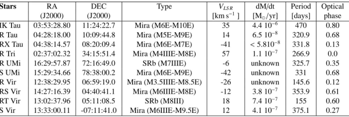
Table 1. (-continued). Stars observed in this work. The stellar type is derived from the literature as are the mass loss rates (e.g.

Loup et al. 1993) and the period (e.g. AAVSO data).

Stars RA DEC Type VLS R dM/dt Period Optical

(J2000) (J2000) [km s−1_] _[M

⊙/yr] [days] phase

IK Tau 03:53:28.80 11:24:22.7 Mira (M6E-M10E) 35 4.4 10−6 ₄₇₀ _0.80

R Tau 04:28:18.00 10:09:44.8 Mira (M5E-M9E) 14 6.5 10−8 _320.9 _0.68

RX Tau 04:38:14.57 08:20:09.4 Mira (M6E-M7E) -41 <5.810−8 _331.8 _0.13

R Tri 02:37:02.32 34:15:51.4 Mira (M4IIIE-M8E) 57 1.1 10−7 _266.9 _0.0

R UMi 16:29:57.87 72:16:49.0 SRb (M7IIIE) -6 unknown 325.7 0.35 S UMi 15:29:34.66 78:38:00.2 Mira (M6E-M9E) -42 unknown 331 0.68 R Vir 12:38:29.95 06:59:19.0 Mira (M3.5IIIE-M8.5E) -26 unknown 145.6 0.12 RS Vir 14:27:16.39 04:40:41.1 Mira (M6IIIE-M8E) -12 3.8 10−7 _353.9 _0.61

RT Vir 13:02:37.96 05:11:08.5 SRb (M8III) 18 7.4 10−7 ₁₅₅ _0.60

S Vir 13:33:00.11 -07:11:41.0 Mira (M6IIIE-M9.5E) 12 4.1 10−7 _375.1 _0.27

SiO (v=1, J=2-1) line observations at 86.243442 GHz were carried out towards 57 stars in August and November 1999 with the IRAM 30m radiotelescope. The pointing was regu-larly checked directly on the star itself (for the vast majority of objects). In order to obtain flat baselines, we used the wobbler switching mode. The system temperature of the SIS receiver ranged from 110 to 170 K. The front-ends were the facility receivers A100 and B100, and the back-end was the autocor-relator. The lines were observed with a spectral resolution of 0.3 km s−1 _{. The integration times were 4-10 minutes using}

the wobbler switching. The forward and main beam efficiencies were respectively 0.92 and 0.77 at 3 mm. (Additional SiO (v=1, J=5-4) line observations at 215.596 GHz were also performed in most stars studied here; results will be reported elsewhere.)

Our source sample (see Table 1) consists of 43 Miras, 7 Semi-Regular stars (hereafter SR), 2 IR late-type stars, 1 irregu-lar variable, 3 supergiants and 1 Planetary Nebula (QX Pup) se-lected from our SiO maser master catalogue (Herpin & Baudry, private communication). Coordinates and the main characteris-tics of the objects are given in Table 1. Nearly 60 % of stars in this table have been observed with the HIPPARCOS satellite and have thus excellent optical positions; such positions have been adopted in our work.

3. Results: Polarization Study 3.1. Individual results

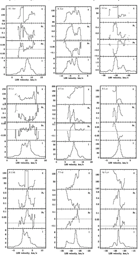
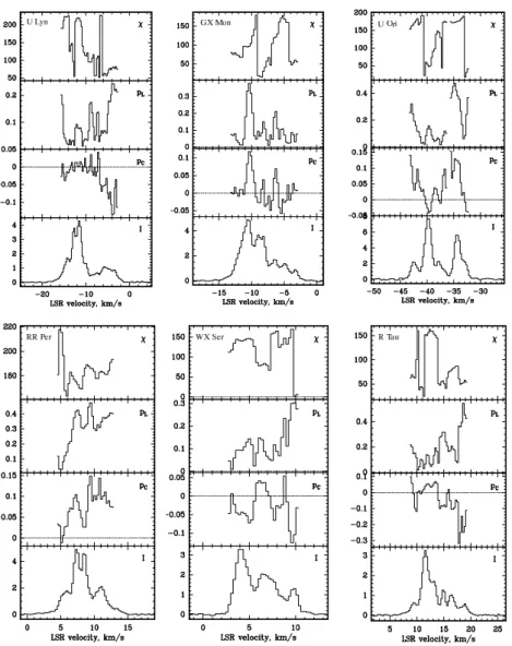
Values of the polarization level presented here (see Table 2) are those measured for the different components within the SiO maser emission profile for each star. Examples are given in Fig.2 for a few stars. The complete Figure 2 with all the observations is available in electronic form at http://www.edpscience.org. Only the well identified compo-nents are considered (distinct peaks or strong wing emission well separated from the bulk emission, according to the noise). Some interesting cases are briefly presented below.

Some profiles show isolated emission red/blue-shifted from the main emission which are more strongly circularly po-larized (e.g. IRAS 18204-1344). These peculiar characteristics imply a different spatial origin for the main and higher/lower velocity components. Sometimes the circular polarization is

regularly varying across the profile (e.g. R Leo), but sometimes not.

In T Lep, the SiO emission shows two peaks linked by a plateau; the circular polarization is linearly varying across the profile from -11 to 10 % (see Fig. 2). Several objects (e.g. S UMi, IK Tau) show the same pCpattern.

The IR late-type source IRAS18158-1527 exhibits a com-plex profile with several well defined components, each of them differently polarized indicating a complex maser structure with probably different maser spots contributing to the whole emis-sion. The red wing emission is highly polarized (43 %). Such a complex multi-component maser line profile and ”semi-circle”, convex, pC pattern appear to be characteristic of SR objects

(see other similar objects in our sample and R Crt in Fig. 2). Nevertheless, the circular polarization pattern observed in the Mira star U Lyn is a convex profile as encountered in SR ob-jects.

One of the most studied Mira star is R Leo. The profile is made of a strong emission with a blue broad line wing. Main and linewing emissions are strongly polarized (respec-tively negative and positive pC ∼ 9 − 10 %). R Leo is a very

well studied object exhibiting a bipolar jet throughout its en-velope. The clear symmetry observed between the positive and negative circular polarization patterns in the main and wing line emissions suggests that the maser emission comes from the jet lobes. We note that the Mira star RS Lib exhibits an emission and polarization pattern similar to that observed in R Leo. R Leo and RS Lib may have the same spatial structure.

3.2. Analysis

The circular polarization level in several of our objects has already been measured by Kemball & Diamond (1997) or Barvainis, McIntosh & Predmore (1987). For TX Cam and W Hya, our results are consistent with previous observations:

– in TX Cam, the bulk of the emission is weakly circularly

polarized while its wings show pC∼ 3 − 6% in good

agree-ment with the VLBI observations of Kemball & Diamond in 1997 who derived an average value of pC∼ 3 − 5%;

– in the Semi-Regular object W Hya, the central emission is

(6)

Fig. 2. Position angle of polarization (χ) in degrees, linear (pL) and circular (pC) polarization levels and intensity (I = T a⋆in

Kelvin; the conversion factor is 6 Jy/K) for the SiO emission observed in several stars.

peaks show pC= 2-6 %), which is consistent with the 5 %

of Barvainis, McIntosh & Predmore (1987).

On the contrary, the circular polarization level we derive in VY CMa, R Cas, R Leo, and VX Sgr is different from levels mea-sured by Barvainis, McIntosh & Predmore (1987), respectively

1-4, 2-6, 9-10 and less than 3 % while they found respectively 6.5, 1.5, 2.4 and 8.7 %. This difference is significant and may be due to variability over the fifteen intervening years. Indeed time variability of the polarization remains an open question in the field. Glenn et al. (2003) have shown that the individ-ual maser feature lifetime ranges from a few months or less to

(7)

Fig. 2. (-continued). Position angle of polarization (χ) in degrees, linear (pL) and circular (pC) polarization levels and intensity

(I = T a⋆_{in Kelvin) for the SiO emission observed in several stars.}

more than 2 years, i.e. the characteristic time over which the Q and U spectral features persist. The average linear polarization is 23 % in Glenn et al. sample with a typical dispersion of 7%. Cotton et al. (2004) have comparable epoch spacing and do not conclude on the variability. Our observations were repeated at intervals of a few months (August and November 1999) and the polarization tends to remain stable between the two epochs.

We emphasize that we cannot spatially distinguish with a single dish radiotelescope between the different maser spots producing the SiO profile (various masers spots contribute in the various features observed at a given velocity). The whole SiO maser emission region, hence all the maser cells, lie within the 29 arcseconds of the 30m (but not necessarily with a uni-form distribution) while the SiO emission covers less than 40 milliarseconds in TX Cam (Kemball & Diamond 1997) and thus everything is beam averaged. This means that any con-clusion on the geometry of the objects observed here would be much uncertain. Only global trends or global geometry can be discussed. One of the consequences of this spatial resolu-tion problem is that if the polarizaresolu-tion vectors are distributed

isotropically around the object, the average polarization level that we measure is zero, even if the maser emission produced in each SiO cell is well polarized.

A global analysis of our data in Table 2 shows the follow-ing. We find that pL varies between 0 and 70 %, and pC

be-tween 0 and ±43 %. Hence, polarization vectors are not dis-tributed isotropically. Emission from Mira-type objects clearly tends to have a relatively high linear ( < pL>Mira ≃ 30%,

<pL>S R≃ 11%) and circular polarization (< pC >Mira≃ 9%,

<pC >S R ≃ 5%). Note that the emission from the PN QX

Pup is highly polarized, and, on the contrary, maser emission from supergiants shows very weak polarization (< pL>=5%,

<pC >=2%), with the exception of one maser component in S

Per. Moreover, all observations show that the polarization level varies across the maser line profile (see Fig. 2), i.e. the differ-ent spectral compondiffer-ents of the maser emission producing the profile are coming from different localizations in the SiO shell and have different polarization levels. The highest polarization level for one object can be encountered either in the main peak, or in the other components.

(8)

Semi-Regular objects (RU Aur, R Crt, W Hya, S Per, AH Sco, R UMi, RT Vir) have a common circular polarization pattern with the central main emission unpolarized and other peak emission or wings being strongly polarized: a characteris-tic ”semi-circle” (i.e. convex shape) pattern for pC is observed

(see R Crt in Fig. 2). The infrared late-type star IRAS18158-1527 exhibits a similar pattern, thus suggesting that this star is a semi-regular.

A group of objects (W And, NV Aur, T Cas, R Com, T Lep, IK Tau, S Ser, S UMi) shows approximately the same pC

pattern (see T Lep in Fig. 2); the circular polarization varies linearly across the line profile from a positive value to a neg-ative one (or the contrary). The only common spectral charac-teristic of the SiO emission from these stars is the presence of an plateau-like emission on top of which the narrow emission peaks are located.

4. Discussion

In this section, we first discuss our source sample in the frame of the 2-color diagram. Then, we briefly summarize the existing SiO maser polarization theories. Finally, we discuss our data set in this context and estimate the stellar magnetic field strength.

4.1. 2-color diagram

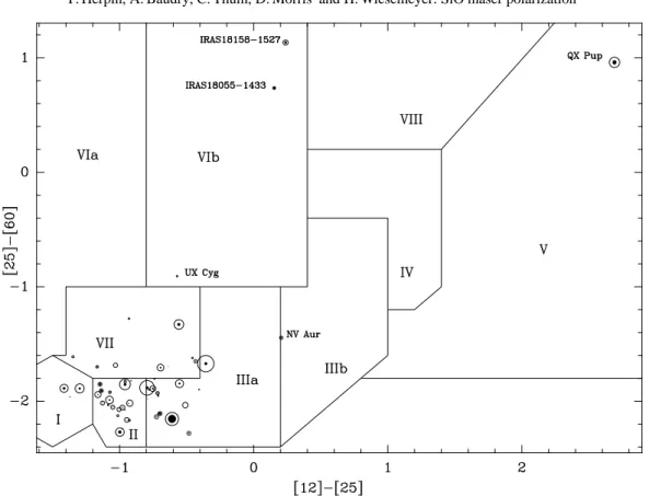
Stars of our sample can be plotted in a [12]-[25], [25]-[60] color-color diagram (van der Veen & Habing 1988; [12], [25] and [60] stand respectively for 12, 25 and 60 microns IRAS-fluxes). This diagram is partitioned into several regions (see Fig. 3) defined by van der Veen & Habing as follows: Region I, oxygen-rich non variable stars without circumstellar shells; Region II, variable stars with young O-rich circumstellar shells; Region IIIa, variable stars with more evolved O-rich circum-stellar shells; Region IIIb, variable stars with thick O-rich cir-cumstellar shells; Region IV, variable stars with very thick O-rich circumstellar shells; Region V, Planetary Nebulae and non-variable stars with very cool envelopes; Region VIa, non vari-able stars with relatively cold dust at large distance; Region VIb, variable stars with relatively hot dust close to the star and relatively cold dust at large distance; Region VII, variable stars with more evolved C-rich circumstellar shells.

On Fig. 3 are represented the linear and circular polariza-tion level for the main SiO emission component from each star. Most of the objects in our sample fall in regions II and IIIa and do not show particular characteristics, except for S Cas (an S-type star) where the circular polarization is high. Mira-type stars are in regions I, II, IIIa and VII. IR late-type objects are in VIb and VII. The SRa semi-regular variable W Hya is in I, while the SRb stars lie in IIIa (RU Aur, RT Vir, R Crt), II (R UMi), and Src in IIIa (S Per) and VII (AH Sco). The Red Supergiants, VY CMa and VX Sgr, and the IR supergiant IRAS 18204-1344 lie in VII. Objects in Region VII do not exhibit strong polarization compared to other objects, perhaps because of their more C-rich circumstellar shells (e.g. AU Aur) or be-cause of the presence of hot dust close to the star implying less SiO abundance and thus weaker emission, making the polar-ization measurement less significant. The presence of hot dust

may also influence the pumping of the SiO molecules and thus the polarization level; the optically thick, hence isotropic, radi-ation field of hot dust can assist the collisional pumping. This could apply to UX Cyg (an irregular variable), IRAS 18055-1433 and IRAS 18158-1527 in region VIb. QX Pup in region V is a PN and exhibits strong polarized emission. Note that IRAS 18055-1433 and IRAS 18158-1527 show very strong circular polarization in their line wings. We may conjecture here that wing emission comes from more outer layers than those where the main line is excited (Herpin et al. 1998); as a consequence, the SiO cells giving rise to wing emission are less influenced by the presence of hot dust (hot dust preferably lies in the inner layers).

4.2. The SiO maser polarization theory

Since SiO is non-paramagnetic, the Zeeman splitting gνB (g

is the Land factor) is much less than the Doppler width. Moreover, the degree of saturation is the ratio of the rate R for stimulated emission to the loss rate Γ (usually Γ is approxi-mated by the inverse radiation lifetime for a vibrational tran-sition, Γ ≃ 5 s−1 _{for SiO masers, Wiebe & Watson 1998).}

Hence, if R ≥ Γ, the maser is saturated. In fact, in the Orion case Plambeck et al. (2003) show that, despite the radiation beam angle is unknown, the 86 GHz SiO maser is saturated. The maser is saturated if the angle averaged intensity J = IΩb 4π (Ωbis the beaming solid angle) is larger than the saturation

in-tensity JS; JS is a theoretical quantity. The saturation depends

on the angle into which the radiation is beamed, but this angle is unknown (Watson & Wyld 2001), thus J cannot be directly measured (even if I is measurable when the maser is resolved, the beaming angle Ω is not an observable).

For more than one decade, two schools have come up against each other to explain SiO maser emission. SiO polar-ization theory is described in: (i) Watson (e.g. Watson & Wyld 2001, Wiebe & Watson 1998, Nedoluha & Watson 1994); (ii) Elitzur (2002, 1998, 1996, 1994).

The main difference between the two approaches rests in the pumping mechanisms. While anisotropic pumping associ-ated with a weak field produces high pLand quite significant pC

in Watson’s model, a strong magnetic field is necessary with the more classical pumping mechanisms used in Elitzur’s model. Details about both models can be found in the Elitzur’s review (2002).

We may summarize the main characteristics of Watson’s model as follows:

– non-Zeeman effect; – anisotropic pumping;

– no direct relation between pC and B. An estimation of B

can only be derived through complete calculation of the radiative transfer. Nevertheless, when maser saturation is not important, the ”thermal” spectral line equation_δ_I/δvV =

αB cos θ is applicable (Fiebig & G¨usten 1989); I is the

in-tensity with respect to Doppler velocity v, θ is the angle between B and the line of sight, α is a constant;

– the Zeeman splitting parameter gΩ (in frequency units

(9)

Fig. 3. Two-color diagram for our sample. The size of the empty and filled circles for each star are proportional to respectively

the linear and absolute circular polarization level measured for the main peak of SiO emission.

– saturated or unsaturated maser (saturated maser increases

pC);

– linear correlation between pL and pC, and high pL is

needed;

– intensity dependent circular polarization;

– B of a few 10 mG varying as r−2,3_{throughout the envelope.}

In contrast with Watson’s work, Elitzur’s model is based on the Zeeman effect and the exponential maser growth in the un-saturated phase; the polarization characteristics are preserved as the radiation is amplified into the saturated regime. This model was improved several times (Elitzur 1994, 1996, 1998) and takes into account the anisotropic pumping. The mag-netic field generates circular polarization and the main pump-ing mechanism for the SiO maser is a ”classical” radiative-collisional process. For saturated masers, a direct relation be-tween pCand B is obtained from simple calculations. The ratio

xBof the Zeeman splitting ∆νB to the Doppler linewidth ∆νD,

can be determined (Elitzur 1996) from vpeak, the ratio of the

Stokes parameter V/I at a given peak feature:

xB=

3√2

16 vpeakcos θ (7)

Following Barvainis, Mc Intosh & Predmore (1987) and Elitzur (1996) we arbitrarily take θ ≃ 45◦

⇒ xB=

3

16 vpeak (8)

⇒ xB= 0.1875 10−2mC (9)

where mC is the polarization fraction in percentage (i.e. 100

pC). Moreover:

xB= 14gλ

B

∆vD

(10) where g is the Land´e factor with respect to the Bohr magneton,

λthe transition wavelength in cm, B the field in Gauss and ∆vD

the Doppler width in kms−1_{. Thus,}

B = 0.1875 10−2 ∆vD

14gλmC (11)

With g ≃ 10−3_{, ∆v}

D= 1 km s−1and λ = 0.2877 cm, we derive:

B ≃ 0.46 mC (12)

This model predicts that there is no correlation between pC

and pL (see also Watson & Wyld 2001); such a mechanism

leads to an inferred magnetic field of a few Gauss to 10 Gauss for the SiO maser zone, the field hence varying as r−1,2_across

the envelope.

4.3. Theory against present observations

The relevance of the two different polarization theories can be assessed via a few observational checks:

– dependence of circular polarization on intensity; – linear correlation between pCand pL;

– Zeeman effect, i.e. spectral shape of the Stokes parameter

(10)

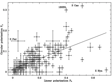
Fig. 4. Absolute fractional polarization pc versus pL for the

whole sample and all maser components (wings + center). A regression fit is shown: pC≃ 0.015 + 0.25pL

– coherence of B strength values inferred from OH and

H2O observations.

As we do not resolve the maser emission into individual spatial components, our current data set is biased by the beam aver-aging. Therefore, some effects cannot be tested with our data. In the Zeeman effect case, the spectral shape of the Stokes pa-rameter V must follow an antisymmetric S curve with sharp re-versal at line center (Elitzur 1996). Unfortunately the doppler width is less than the resolution of the observations and we cannot conclude.

We may look for any correlation between pC and pL. As

shown in Figs. 2 and 3, it first appears that in all cases pLis

larger than pC as is predicted by all models. More precisely,

pC is noticeable if and only if pL is high. If we plot the

val-ues of pC and pL derived for all maser components in this

work (Fig. 4) and make a regression fit to our data we obtain

pC ≃ 0.015 + 0.25 pL. The circular polarization level tends

to vary approximately linearly with pLin agreement with the

fact that no pC is detected towards sources with a marginal pL

detection. Note that in Fig. 4, four objects, S Per, IRAS18055-1433, S Cas and χ Hya, do not follow the same general trend observed for the rest of the sample. (The case of the Supergiant S Per, however, is an exception as it exhibits substantial pC

while pL <pC.) This observation may in fact favour Watson’s

model. It must be stressed again that the beam-averaged po-larization that we measure makes any conclusion uncertain. In fact, due to this averaging, we should observe no correlation at all, even if such one would exist !

As mentioned earlier (see Section 3.2) we observe relatively high circular polarization rates in several stars (< pC>Mira ≃ 9%, < pC>S R ≃ 5%). These values are larger

than those predicted from Watson’s model (e.g. Nedoluha & Watson 1994). We also have not been able to find any cor-relation of pC with total intensity. Finally, although we adopt

the Zeeman case to derive the magnetic field strength (see Section 4.5), we cannot conclude firmly from present obser-vations which maser theory prevails for SiO emission.

4.4. Magnetic field in AGB stars

A better knowledge of the stellar magnetic field strength is cru-cial to understand the last stages in the life of an Asymptotic Giant Branch (hereafter AGB) star. These stages are charac-terized by a high mass loss process driven by the radiation pressure; they are also influenced by the magnetic field (Palen & Fix 2000, Blackman, Frank & Welch 2001, and references therein). A strong magnetic field may rule the mass loss geom-etry; in particular, it could be the cause of a higher or lower mass-loss rate in the equatorial plane (Soker 2002), and thus determine the global shaping of these objects. But, as the di-rect dynamical effect of the magnetic activity is much lower than that of the wind (although in local spots the magnetic field can be dominant), the role of the magnetic field might be indirect. Moreover, the observed high mass loss rates are hardly explained by a single process and need a combination of several factors such as rotation, the presence of a compan-ion (binary stars, with our without common envelope, exhibit-ing mass transfer or tidal effects are common; Soker 1997) and a magnetic field. During its quick transition to the PN stage, the AGB star will completely change its geometry: the quasi-spherical object becomes axisymmetrical, point-like symmet-rical or even shows higher order symmetries (Johnson & Jones 1991, Sahai & Trauger 1998, Balick & Frank 2002). The clas-sical or generalized Interacting Stellar Winds (hereafter ISW or GISW) models (Kwok 2000, Soker & Livio 1989, Morris 1987) try to explain this shaping, but have serious difficulties in producing complicated structures with peculiar jets or ansae (e.g., CRL 2688, Delamarter 2000) and do not fully address the origin of the wind. Furthermore, recent X-ray studies with the Chandra satellite do not completely agree with GISW predic-tions for temperatures (Guerrero et al. 2001).

Some recent studies tend to demonstrate the importance of the magnetic field in evolved objects. Bujarrabal et al. (2001) show that for 80% of the PPNe in their sample the fast molec-ular flows have too high momenta to be powered by radiation pressure only (1000 times larger in some cases) what may be explained by magnetic field. Moreover, X-ray emission found in evolved stars (e.g. H¨unch, Schmitt & Schr¨oder 1998) may indicate the presence of a hot corona that possibly results from magnetic activity. Very recently, magnetic field was discovered for the first time in central stars of PN (Jordan et al. 2005) and estimated to kiloGauss, much stronger than what we find here from our SiO data in QX Pup.

New models involving the magnetic field have been devel-oped trying to explain the morphology changes of an object during its transition from the AGB stage to the PN stage; B plays the role of a catalyst and of a collimating agent. The most simple models are based on a moderately weak magnetic field alone (B ≃ 1 Gauss at the stellar surface, a few 1013_{cm, i.e.} at a radiis of a few AU, Soker 1998). The influence of B is stressed by the work of Smith et al. (2001) and Greaves (2002) in VY CMa. But the role of B can only be decisive when its en-ergy density is greater than the radiative pressure, i.e. when B is greater than around 10 G close to the stellar surface in the SiO region (see Soker & Zaobi, 2002). Arguing that such a strong field may be very unusual, Balick & Frank (2002) explain that

(11)

B alone cannot produce the observed structures, and a com-bination of several factors has thus to be considered (rotation, magnetic field and presence of a companion).

Soker & Harpaz (1992) first proposed a model with a weak magnetic field (≤ 1 G) and included a slow rotation together with the presence of a companion to transform the envelope (and lead for example to the peculiar geometry observed in NGC 6826 or NGC 6543). Even if the star were not binary, the influence of B is probably important locally (Palen & Fix 2000). A significant magnetic field can form cold spots on the star’s surface and a slow rotation of the star can then increase the field strength to build up a dipolar magnetic field varying as 1/r3_{(Matt et al. 2000); such a field is stronger at the equator} and may thus lead to an axisymmetrical mass loss.

The main argument against the dominant influence of the magnetic field on the shaping of the circumstellar enve-lope is that a strong field seems to be necessary to dominate the dynamics of the gas. However, several authors (Pascoli 1985, 1992, 1997, Chevalier & Luo 1994, Garc´ıa-Segura 1997, Gurzadyan 1997, Delamarter 2000) have demonstrated the strong influence of a reasonable toro¨ıdal magnetic field em-bedded in the normal radiation-driven stellar wind (Magnetic

Wind Bubble theory, hereafter MWB). This field has a strength

between a few Gauss and a few 10 Gauss at a few stellar radii (the SiO region is believed to be at ∼ 1014

cm or ∼ 7 − 10 AU), varies as 1/r2

, then as 1/r at larger radii; therefore B ∼ 1 mG at 1016,17cm or 700-7000 AU. These results are confirmed by the simulations of Garc´ıa-Segura, Lopez & Franco (2001) for the PN He 2-90. Even if the origin of the wind is not explained by these models, it seems clear that a magnetic field is essential to generate fast collimated outflows (Kastner et al. 2003).

There are many models of magnetic jet production and col-limation and some, or all of them, are applicable to various star geometries. One most interesting study was performed by Blackman, Frank & Welch (2001) in which the magnetic field emerges from the AGB stellar core and the resulting 1G field helps to collimate the radiation-driven wind or a stronger, more anisotropic, magnetically driven wind.

4.5. Magnetic field in our sample

The exact interpretation, in terms of magnetic field, of our ob-servations depends on the adopted specific SiO maser model (see Sections 4.2 and 4.3). From the current knowledge of the strength of the magnetic field in the OH and H2O layers we ex-pect B//of a few Gauss at least in the SiO maser region (see

also Kemball & Diamond 1997), i.e. at 5-10 AU from the cen-tral object. This tends to invalidate Watson’s model, and fur-thermore tends to agree with a field varying in r−1,2 _as

pre-dicted by Elitzur’s model. However, Vlemmings et al. (2005) measured the circular polarization of the H2O maser emission in a few evolved stars with the VLBA observations and showed that the magnetic field is either a solar-type field (with a r−2

field strength dependence) or a dipole magnetic field (with a

r−3_{dependence) in their sample.}

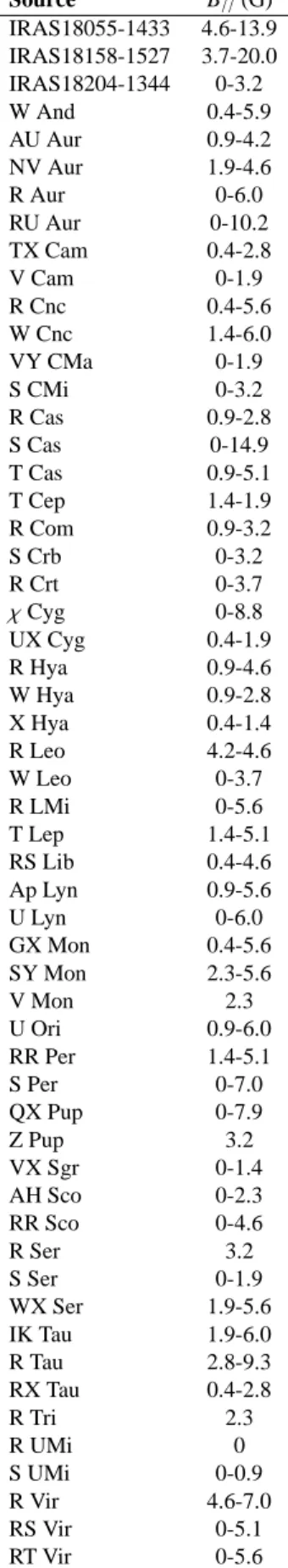
In the following, we decide to use Elitzur’s theory (Zeeman case) to infer magnetic field strength from the circular

polar-ization levels. From equation (12), we thus calculate the mean value of the magnetic field B//for each star and give results in

Table 3.

For our sample B//is between 0 and 20 Gauss, with a mean

value of 3.5 G. This value combined with the strength of the field in more outer layers of the envelope (OH and H2O masers) agrees with a B field variation law in 1/r, closer to Elitzur’s model. As explained in the Introduction and in Section 4.4, B alone can be the main agent to shape the circumstellar enve-lope if its value is larger than around 10 Gauss. This means that only S Cas, RU Aur, IRAS 18055-1433 and IRAS 18158-1527 may have a magnetic field ruled geometry (B > 10 G in these objects). The rest of our sample shows that B is sufficiently strong to be dominant at this stage of the AGB star evolution, but it should be associated with rotation and the presence of a companion as suggested in models mentioned in Section 4.4. Despite our B measurements are beam averaged, they suggest in many cases that they are not too much (not orders of mag-nitude) below the critical value; local B values may exceed in many cases the critical value, and therefore participate in the shaping of the AGB envelopes. Our estimated values of B are consistent with the MWB theory (toro¨ıdal magnetic field) or the model of Blackman, Frank & Welch (2001).

From Elitzur (1996) and our measurements < pC>Mira ≃

9%, < pC>S R≃ 5%, we can estimate (see Eq. (9) in Sect. 4.2)

that < xB >is around 0.017 and 9.4 10−3respectively for

Mira-type objects and semi-regular variables. Moreover, according to Elitzur (1996, see Fig.2), there is no stationary physical solu-tions for propagation at sin2θ < 1₃(i.e. at sin2θ < 1₃the radiation is not polarized). As xBis small (< 0.02), from Fig.2 of Elitzur

(1996) we can estimate the volume of phase space in which propagation of linear polarization in a maser is possible or not (θ > 35.3◦_{or θ < 35.3}◦_{); we then calculate that the probability}

for a random magnetic axis to be aligned with a given direction (our line of sight) is better than 35.3◦_{. Our present estimate}

is that around 18 %. Therefore, Elitzur’s model predicts that 18.4 % of the SiO 86 GHz masers should not be linearly po-larized, because such polarized masers cannot propagate if the magnetic field, although weak, is closer than 35.3◦_{to the line of}

sight (propagation direction). Hence non polarized maser emis-sions do not imply no or weak magnetic field. In our sample, roughly 13 % of the SiO maser components have no detectable or very weak (< 3%) polarization.

We looked without success for a possible correlation be-tween the polarization rates and physical parameters such as the known envelope asymmetry, the presence of SiO maser high velocity linewings (see Herpin et al. 1998), or the mass loss rate. If the magnetic field plays an important role in the shaping of the object, one may expect to find a relationship be-tween the strength of B// (thus pC) and the geometry of the

object. Unfortunately, no trend is clearly found in our data. Nevertheless it is known that radiative pressure is driving the wind in AGB objects and it is thus not surprising that we find no correlation between the B strength and a known asymmetry in our sample. Of course, our stellar sample would require new observations with sufficient spatial resolution (VLBI) to con-firm the present results; the same type of study should also be conducted toward several Proto-PN and PN objects.

(12)

5. Conclusion

We have made a study of the SiO maser polarization in a repre-sentative sample of evolved stars, simultaneously measuring, for the first time, the 4 Stokes parameters. From our mea-surements we derive the circular and linear polarization lev-els and shows that, due to the beam averaging of our polar-ization measurements, we cannot firmly discriminate between the two dominant theories of SiO maser emission. In partic-ular, VLBI observations of our source sample are absolutely necessary to distinguish between Zeeman or non-Zeeman the-ories. Nevertheless, the magnetic field strength was derived assuming Elitzur’s model. B varies between 0 and 20 Gauss, with a mean value of 3.5 G. As a consequence, we suggest that the magnetic field plays a significant role in the evolu-tion of these objects. Within the frame of the Zeeman theory the magnetic field could shape or even collimate the gas lay-ers surrounding the AGB objects. Emission from Mira-type ob-jects clearly tends to have a higher linear ( < pL>Mira ≃ 30%,

<pL>S R≃ 11%) and circular polarization (< pC>Mira ≃ 9%,

<pC >S R ≃ 5%). Basically, if there is a real correlation

be-tween pCand the strength of the magnetic field, this trend may

indicate that the magnetic field may be stronger in Mira objects than in Semi-Regular variables (at least in the inner layers of the circumstellar envelope).

To better understand the mechanisms at work with the mag-netic field, complementary studies have to be conducted and in particular the presence of a companion has to be investigated in a large sample of objects. Of course VLBI maps of the mag-netic field in these stars are essential. Another important objec-tive is to investigate the evolution of the magnetic field and its influence during the transition from the AGB star phase to the PN stage.

Acknowledgements. The authors are grateful to M. Elitzur for

read-ing and commentread-ing on this paper. We also thank W.D. Watson for his useful comments and suggestions. The authors are indebted to the staff of the IRAM 30m telescope who most efficiently helped during the observations and to R. Mauersberger who closely followed part of these observations. Finally, we also thank the referee for several useful comments.

References

Balick B., Frank A. 2002, ARAA 40, 439

Barvainis R., McIntosh G., Read Predmore C. 1987, Nature 329, 613 Blackman E.G., Frank A., Welch C. 2001, ApJ 546, 288

Bujarrabal V., Castro-Carrizo A., Alcolea J., S´anchez Contreras C. 2001, A&A 377, 868

Bujarrabal V. 2003, Mass-losing pulsating stars and their circum-stellar matter, edited by Y. Nakada, M. Honma and M. Seki. Astrophysics and Space Science Library, Vol. 283, Dordrecht: Kluwer Academic Publishers, p. 275 - 282

Chevalier R.A., Luo D. 1994, ApJ 435, 815

Cotton W.D., Mennesson B., Diamond P.J. et al. 2004, A&A 414, 275 Delamarter G.R. 2000, Ph-D thesis, University of Rochester

Elitzur M. 1994, ApJ 422, 751 Elitzur M. 1996, ApJ 457, 415 Elitzur M. 1998, ApJ 504, 390

Elitzur M. 2002, Astrophysical spectropolarimetry, Proceedings of the XII Canary Islands Winter School of Astrophysics, edited by J. Trujillo-Bueno, F. Moreno-Insertis, and F. Snchez. Cambridge, UK: Cambridge University Press, p. 225 - 264

Fiebig D., G¨usten R. 1989, A&A 214, 333 Garc´ıa-Segura G. 1997, ApJ 489, L189

Garc´ıa-Segura G, Lopez J.A. & Franco J. 2001, ApJ 560, 928 Glenn J., Jewell P.R., Fourre R., Miaja L. 2003, ApJ 588, 478 Goldreich P., Keeley D.A., Kwan J.Y. 1973, ApJ 179, 111 Greaves J.S. 2002, A&A 392, L1

Guerrero M.A., Chu Y., Gruendl R.A. et al. 2001, ApJ 553, L55 Gurzadyan G.A. 1997, in The Physics and Dynamics of Planetary

Nebulae, Berlin/Heidelberg/New York: Springe-Verlag

Herpin F., Baudry A., Alcolea J., Cernicharo J. 1998, A&A 334, 1037 Herwig F. 2003, Planetary Nebulae: Their Evolution and Role in the Universe, Proceedings of the 209th Symposium of the International Astronomical Union, edited by Sun Kwok, Michael Dopita, and Ralph Sutherland, p.61

H¨unch M., Schmitt J.H.M.M., Scrh¨oder K.-P. 1998, A&A 330, 225 Jordan S., Werner K., O’Toole S.J. 2005, A&A 432, 273

Johnson D.R., Clark F.O. 1975, ApJ 197, L69 Johnson J.J., Jones T.J. 1991, AJ 101, 1735

Kastner J.H., Balick B., Blackman E.G. et al. 2003, ApJ 591, L37 Kemball A.J., Diamond P.J. 1997 ApJ 481, L111

Kwok S. 2000, in The origin and Evolution of Planetary Nebulae, Cambridge Astrophysics Series 31, Cambridge University Press edition

Loup C., Forveille T., Omont A., PAul J.-F. 1993, A&ASS 99, 291 McIntosh G.C., Predmore C.R., Moran J.M. et al. 1989, ApJ 337, 934 McIntosh G.C., Predmore C.R., Patel N.A. 1994, ApJ 428, L29 Matt S., Balick B., Winglee R., Goodson A. 2000, ApJ 545, 965 Monnier J.D., Millan-Gabet R., Tuthill P.G. et al. 2004, ApJ 605, 436 Morris M. 1987, PASP 99, 1115

Nedoluha G.E., Watson W.D. 1994, ApJ 423, 394 Palen S., Fix J.D. 2000, ApJ 531, 391

Pascoli G. 1985, A&A 147, 257 Pascoli G. 1992, PASP 104, 350 Pascoli G. 1997, ApJ 489, 946

Plambeck R.L., Wright M.C.H., Rao R. 2003, ApJ 594, 911 Rowan-Robinson M., Harris S. 1983, MNRAS 202, 767 Sahai R., Trauger J.T. 1998, AJ 116, 1357

Smith N., Humphreys R.M., Davidson K. et al. 2001, ApJ 121, 1111 Soker N., Livio M. 1989, ApJ 339, 268

Soker N., Harpaz A. 1992, PASP 104, 923 Soker N. 1997, ApJS 112, 487

Soker N. 1998, MNRAS 299, 1242 Soker N., Zoabi E. 2002, MNRAS 329, 204 Soker N. 2002, MNRAS 337, 1038

Szymczak M., Cohen R.J. 1997, MNRAS 288, 945

Thum C., Wiesemeyer H., Morris D., Navarro S., Torres M. 2003

Proc. S.P.I.E., 4843, 272

Troland T.H., Heiles C., Johnson D.R., Clark F.O. 1979, ApJ 232, 143 van der Veen W.E.C.J., Habing H.J. 1988, A&A 194, 125

Vlemmings W., Diamond P.J., van Langevelde H.J. 2001, A&A 375, L1

Vlemmings W., van Langevelde H.J., Diamond P.J. 2005, A&A 434, 1029

Wallin B.K., Watson W.D. 1997, ApJ 481, 832 Watson W.D., Wyld H.W. 2001, ApJL 558, 55 Wiebe D.S., Watson W.D. 1998, ApJL 503, 71

(13)

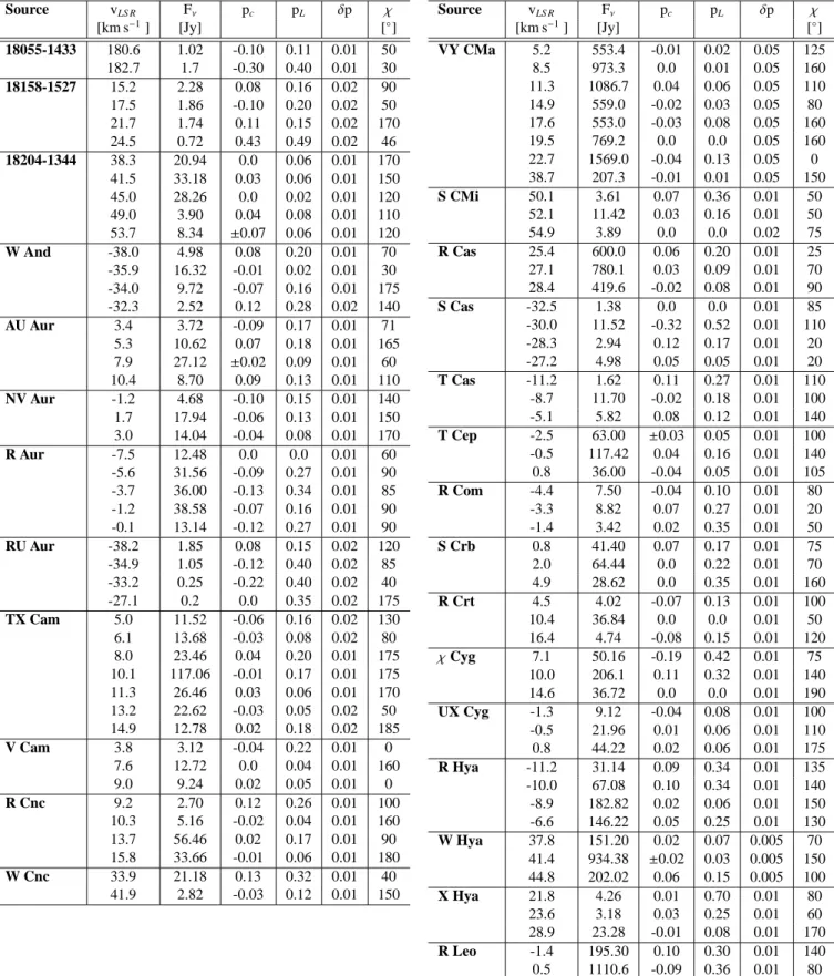
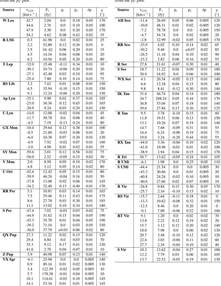
Table 2. Derived parameters of the different components of

the SiO maser emission profile for each star. Only the well identified components are given (distinct peak or strong wing emission separated from the bulk emission). Note that the po-larization is fractional. The δP is the rms derived from the pC

plot. Source vLS R Fν pc pL δp χ [km s−1_] _[Jy] _[◦_] 18055-1433 180.6 1.02 -0.10 0.11 0.01 50 182.7 1.7 -0.30 0.40 0.01 30 18158-1527 15.2 2.28 0.08 0.16 0.02 90 17.5 1.86 -0.10 0.20 0.02 50 21.7 1.74 0.11 0.15 0.02 170 24.5 0.72 0.43 0.49 0.02 46 18204-1344 38.3 20.94 0.0 0.06 0.01 170 41.5 33.18 0.03 0.06 0.01 150 45.0 28.26 0.0 0.02 0.01 120 49.0 3.90 0.04 0.08 0.01 110 53.7 8.34 _±0.07 0.06 0.01 120 W And -38.0 4.98 0.08 0.20 0.01 70 -35.9 16.32 -0.01 0.02 0.01 30 -34.0 9.72 -0.07 0.16 0.01 175 -32.3 2.52 0.12 0.28 0.02 140 AU Aur 3.4 3.72 -0.09 0.17 0.01 71 5.3 10.62 0.07 0.18 0.01 165 7.9 27.12 _±0.02 0.09 0.01 60 10.4 8.70 0.09 0.13 0.01 110 NV Aur -1.2 4.68 -0.10 0.15 0.01 140 1.7 17.94 -0.06 0.13 0.01 150 3.0 14.04 -0.04 0.08 0.01 170 R Aur -7.5 12.48 0.0 0.0 0.01 60 -5.6 31.56 -0.09 0.27 0.01 90 -3.7 36.00 -0.13 0.34 0.01 85 -1.2 38.58 -0.07 0.16 0.01 90 -0.1 13.14 -0.12 0.27 0.01 90 RU Aur -38.2 1.85 0.08 0.15 0.02 120 -34.9 1.05 -0.12 0.40 0.02 85 -33.2 0.25 -0.22 0.40 0.02 40 -27.1 0.2 0.0 0.35 0.02 175 TX Cam 5.0 11.52 -0.06 0.16 0.02 130 6.1 13.68 -0.03 0.08 0.02 80 8.0 23.46 0.04 0.20 0.01 175 10.1 117.06 -0.01 0.17 0.01 175 11.3 26.46 0.03 0.06 0.01 170 13.2 22.62 -0.03 0.05 0.02 50 14.9 12.78 0.02 0.18 0.02 185 V Cam 3.8 3.12 -0.04 0.22 0.01 0 7.6 12.72 0.0 0.04 0.01 160 9.0 9.24 0.02 0.05 0.01 0 R Cnc 9.2 2.70 0.12 0.26 0.01 100 10.3 5.16 -0.02 0.04 0.01 160 13.7 56.46 0.02 0.17 0.01 90 15.8 33.66 -0.01 0.06 0.01 180 W Cnc 33.9 21.18 0.13 0.32 0.01 40 41.9 2.82 -0.03 0.12 0.01 150

Table 2. (-continued). Derived parameters of the different components of the SiO maser emission profile for each star. Only the well identified components are given (distinct peak or strong wing emission separated from the bulk emission). Note that the polarization is fractional. The δP is the rms derived from the pCplot.

Source vLS R Fν pc pL δp χ [km s−1_] _[Jy] _[◦_] VY CMa 5.2 553.4 -0.01 0.02 0.05 125 8.5 973.3 0.0 0.01 0.05 160 11.3 1086.7 0.04 0.06 0.05 110 14.9 559.0 -0.02 0.03 0.05 80 17.6 553.0 -0.03 0.08 0.05 160 19.5 769.2 0.0 0.0 0.05 160 22.7 1569.0 -0.04 0.13 0.05 0 38.7 207.3 -0.01 0.01 0.05 150 S CMi 50.1 3.61 0.07 0.36 0.01 50 52.1 11.42 0.03 0.16 0.01 50 54.9 3.89 0.0 0.0 0.02 75 R Cas 25.4 600.0 0.06 0.20 0.01 25 27.1 780.1 0.03 0.09 0.01 70 28.4 419.6 -0.02 0.08 0.01 90 S Cas -32.5 1.38 0.0 0.0 0.01 85 -30.0 11.52 -0.32 0.52 0.01 110 -28.3 2.94 0.12 0.17 0.01 20 -27.2 4.98 0.05 0.05 0.01 20 T Cas -11.2 1.62 0.11 0.27 0.01 110 -8.7 11.70 -0.02 0.18 0.01 100 -5.1 5.82 0.08 0.12 0.01 140 T Cep -2.5 63.00 ±0.03 0.05 0.01 100 -0.5 117.42 0.04 0.16 0.01 140 0.8 36.00 -0.04 0.05 0.01 105 R Com -4.4 7.50 -0.04 0.10 0.01 80 -3.3 8.82 0.07 0.27 0.01 20 -1.4 3.42 0.02 0.35 0.01 50 S Crb 0.8 41.40 0.07 0.17 0.01 75 2.0 64.44 0.0 0.22 0.01 70 4.9 28.62 0.0 0.35 0.01 160 R Crt 4.5 4.02 -0.07 0.13 0.01 100 10.4 36.84 0.0 0.0 0.01 50 16.4 4.74 -0.08 0.15 0.01 120 χCyg 7.1 50.16 -0.19 0.42 0.01 75 10.0 206.1 0.11 0.32 0.01 140 14.6 36.72 0.0 0.0 0.01 190 UX Cyg -1.3 9.12 -0.04 0.08 0.01 100 -0.5 21.96 0.01 0.06 0.01 110 0.8 44.22 0.02 0.06 0.01 175 R Hya -11.2 31.14 0.09 0.34 0.01 135 -10.0 67.08 0.10 0.34 0.01 140 -8.9 182.82 0.02 0.06 0.01 150 -6.6 146.22 0.05 0.25 0.01 130 W Hya 37.8 151.20 0.02 0.07 0.005 70 41.4 934.38 _±0.02 0.03 0.005 150 44.8 202.02 0.06 0.15 0.005 100 X Hya 21.8 4.26 0.01 0.70 0.01 80 23.6 3.18 0.03 0.25 0.01 60 28.9 23.28 -0.01 0.08 0.01 170 R Leo -1.4 195.30 0.10 0.30 0.01 140 0.5 1110.6 -0.09 0.36 0.01 80

(14)

Source vLS R Fν pc pL δp χ [km s−1_] _[Jy] _[◦_] W Leo 42.7 2.04 0.0 0.18 0.05 170 44.6 2.76 0.0 0.10 0.05 100 47.9 3.30 0.0 0.20 0.05 170 54.2 4.62 0.08 0.42 0.02 35 R LMi 0.3 61.98 0.0 0.02 0.01 25 2.2 52.80 0.12 0.36 0.01 0 3.5 34. 62 0.06 0.20 0.01 15 4.5 14.16 0.04 0.08 0.01 20 6.2 10.56 0.05 0.20 0.01 80 T Lep -32.0 15.48 -0.11 0.34 0.01 10 -30.1 10.74 -0.06 0.20 0.01 20 -27.1 42.48 0.03 0.10 0.01 95 -25.4 7.80 0.10 0.14 0.01 75 RS Lib 3.2 7.62 0.01 0.08 0.01 150 6.5 35.94 -0.10 0.15 0.01 150 9.1 12.24 -0.06 0.20 0.01 150 Ap Lyn -25.1 9.90 0.02 0.37 0.01 185 -23.0 36.36 0.12 0.65 0.01 165 -20.9 9.24 0.03 0.20 0.01 150 U Lyn -14.0 12.00 -0.02 0.04 0.01 45 -11.7 30.78 0.0 0.08 0.01 40 -4.5 7.19 -0.13 0.24 0.01 80 GX Mon -10.4 29.64 0.12 0.38 0.01 100 -8.5 21.60 -0.03 0.08 0.01 20 -6.4 10.38 0.07 0.20 0.01 120 -4.9 7.92 -0.02 0.07 0.01 160 -3.0 4.98 0.01 0.02 0.01 55 SY Mon -59.6 3.01 0.12 0.58 0.02 75 -56.0 2.52 -0.05 0.15 0.02 30 V Mon 2.0 8.58 0.05 0.10 0.02 170 4.8 3.12 0.05 0.14 0.02 80 U Ori -42.4 12.42 0.05 0.15 0.01 80 -39.9 46.26 -0.04 0.16 0.01 50 -37.8 13.08 0.02 0.06 0.01 145 -34.2 32.40 0.13 0.40 0.01 170 RR Per 5.1 10.81 0.03 0.14 0.01 165 7.5 29.46 0.11 0.43 0.01 175 8.6 27.78 0.03 0.30 0.01 185 11.1 13.02 0.10 0.34 0.01 180 S Per -47.4 7.02 -0.03 0.03 0.02 75 -44.9 31.62 0.15 0.04 0.05 190 -43.3 35.70 0.01 0.04 0.05 190 -39.2 71.16 0.0 0.03 0.05 150 -36.0 37.79 _±0.03 0.06 0.02 80 QX Pup 27.3 11.22 0.02 0.15 0.01 120 29.4 6.84 0.0 0.03 0.01 70 35.3 9.12 0.17 0.41 0.01 120 41.6 2.70 0.04 0.07 0.01 10 Z Pup 3.9 40.98 0.07 0.23 0.01 140 VX Sgr -6.1 25.98 0.0 0.0 0.005 140 0.9 89.16 0.01 0.02 0.005 130 3.4 122.39 -0.02 0.05 0.005 10 5.7 178.38 -0.01 0.04 0.005 10 10.1 114.61 -0.03 0.10 0.005 145 14.1 53.34 0.01 0.01 0.005 145 16.2 80.04 0.01 0.02 0.005 160

Source vLS R Fν pc pL δp χ [km s−1_] _[Jy] _[◦_] AH Sco -11.4 26.69 0.05 0.06 0.005 120 -10.0 48.31 0.01 0.02 0.005 120 -7.2 78.78 0.0 0.0 0.005 150 -4.7 54.74 0.0 0.02 0.005 20 -2.8 32.99 -0.02 0.05 0.005 170 RR Sco -33.9 4.02 0.10 0.14 0.02 65 -30.2 9.48 0.0 ±0.07 0.02 85 -26.5 11.16 0.04 0.10 0.02 90 -23.2 2.82 0.06 0.16 0.02 55 R Ser 27.8 21.61 -0.07 0.30 0.01 40 S Ser 18.7 11.22 0.04 0.09 0.01 180 20.9 16.92 0.0 0.06 0.01 100 WX Ser 4.1 20.34 -0.05 0.15 0.01 140 6.6 12.18 0.04 0.15 0.01 80 9.8 8.41 -0.12 0.30 0.01 140 IK Tau 31.6 46.74 0.04 0.14 0.01 180 34.7 288.24 0.05 0.16 0.01 170 36.8 53.04 0.07 0.18 0.01 140 39.6 27.84 0.13 0.36 0.01 125 R Tau 9.5 3.78 -0.10 0.15 0.01 60 11.8 19.51 0.06 0.13 0.01 150 13.1 10.26 0.07 0.19 0.01 140 14.7 7.68 -0.09 0.31 0.01 55 16.4 6.24 -0.08 0.19 0.01 75 19.0 3.24 -0.20 0.44 0.01 55 RX Tau -44.0 3.36 -0.06 0.10 0.02 120 -41.0 10.98 -0.01 0.01 0.02 100 -38.9 2.94 0.04 0.15 0.02 170 R Tri 56.7 13.62 -0.05 0.24 0.01 105 R UMi -6.1 1.98 0.0 0.25 0.05 110 S UMi -44.4 21.54 0.0 0.0 0.005 30 -43.3 30.66 0.0 0.01 0.005 20 -40.8 24.24 -0.02 0.10 0.005 10 -40.0 27.66 0.02 0.07 0.005 10 R Vir -26.8 0.84 0.15 0.30 0.05 170 -25.7 2.16 -0.10 0.15 0.02 10 RS Vir -15.7 2.64 -0.11 0.18 0.01 0 -13.3 10.62 -0.08 0.32 0.01 150 -12.5 8.46 0.0 0.20 0.01 0 -9.1 7.08 -0.06 0.52 0.01 160 RT Vir 9.1 1.20 0.0 0.02 0.02 70 13.8 2.22 0.12 0.19 0.02 20 15.7 3.12 0.12 0.20 0.02 140 18.0 7.98 0.0 0.06 0.02 130 20.7 3.48 -0.10 0.12 0.02 120 22.6 3.03 -0.06 0.11 0.02 60 27.7 2.34 -0.04 0.10 0.02 40 S Vir 10.3 13.62 -0.04 0.27 0.01 180 12.2 7.79 0.03 0.06 0.01 105 13.7 22.52 -0.05 0.19 0.01 130

(15)

Table 3. Average magnetic field strengths derived from pC. Source B//(G) IRAS18055-1433 4.6-13.9 IRAS18158-1527 3.7-20.0 IRAS18204-1344 0-3.2 W And 0.4-5.9 AU Aur 0.9-4.2 NV Aur 1.9-4.6 R Aur 0-6.0 RU Aur 0-10.2 TX Cam 0.4-2.8 V Cam 0-1.9 R Cnc 0.4-5.6 W Cnc 1.4-6.0 VY CMa 0-1.9 S CMi 0-3.2 R Cas 0.9-2.8 S Cas 0-14.9 T Cas 0.9-5.1 T Cep 1.4-1.9 R Com 0.9-3.2 S Crb 0-3.2 R Crt 0-3.7 χCyg 0-8.8 UX Cyg 0.4-1.9 R Hya 0.9-4.6 W Hya 0.9-2.8 X Hya 0.4-1.4 R Leo 4.2-4.6 W Leo 0-3.7 R LMi 0-5.6 T Lep 1.4-5.1 RS Lib 0.4-4.6 Ap Lyn 0.9-5.6 U Lyn 0-6.0 GX Mon 0.4-5.6 SY Mon 2.3-5.6 V Mon 2.3 U Ori 0.9-6.0 RR Per 1.4-5.1 S Per 0-7.0 QX Pup 0-7.9 Z Pup 3.2 VX Sgr 0-1.4 AH Sco 0-2.3 RR Sco 0-4.6 R Ser 3.2 S Ser 0-1.9 WX Ser 1.9-5.6 IK Tau 1.9-6.0 R Tau 2.8-9.3 RX Tau 0.4-2.8 R Tri 2.3 R UMi 0 S UMi 0-0.9 R Vir 4.6-7.0 RS Vir 0-5.1 RT Vir 0-5.6 S Vir 1.4-2.3

(16)

(17)

Fig. 2. Position angle of polarization (χ) in degrees, linear (pL) and circular (pC) polarization levels and intensity (I = T a⋆in

(18)

(19)

(20)

(21)

(22)

(23)